Around View Monitoring-Based Vacant Parking Space Detection and Analysis


Abstract
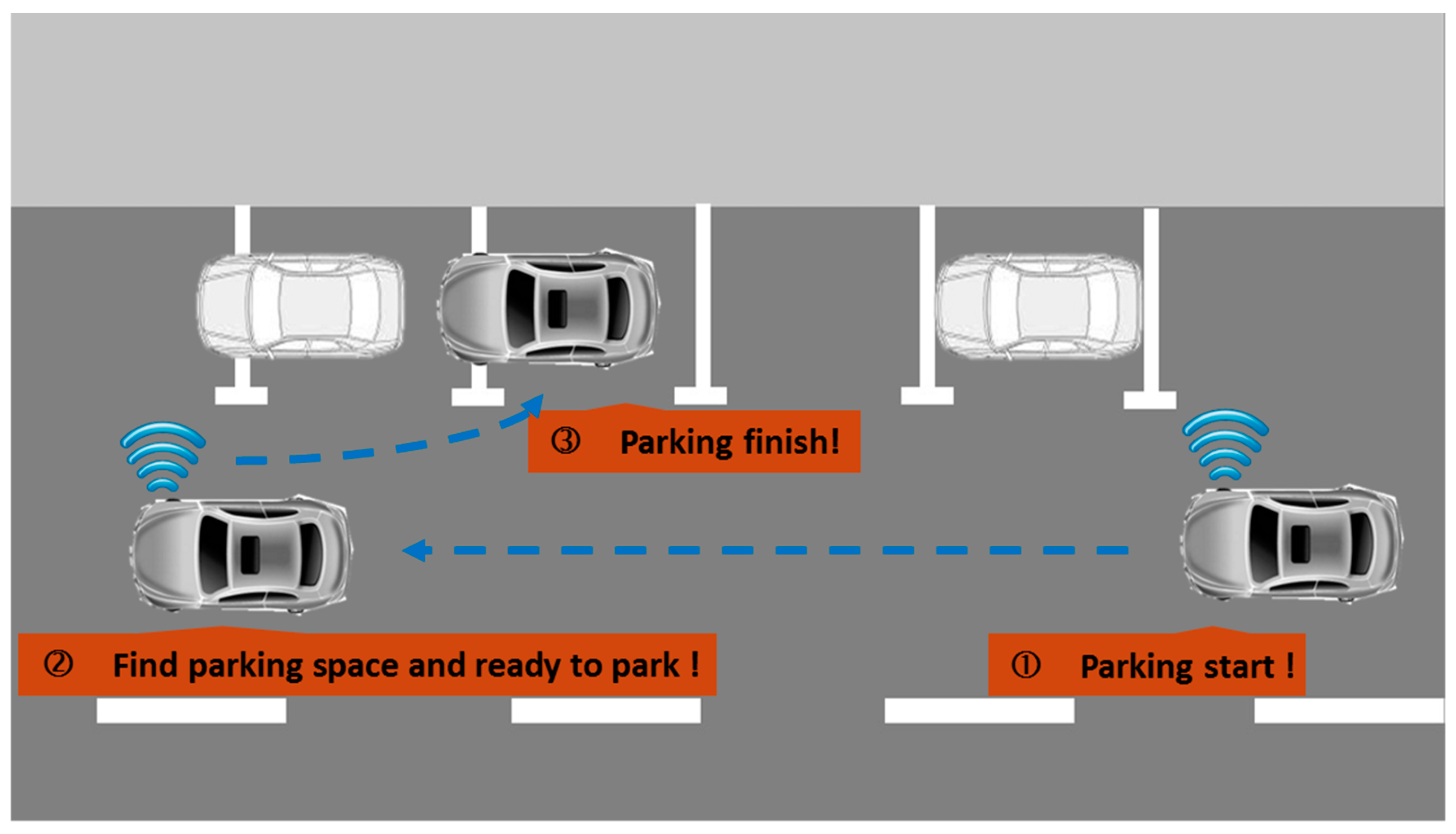
:1. Introduction
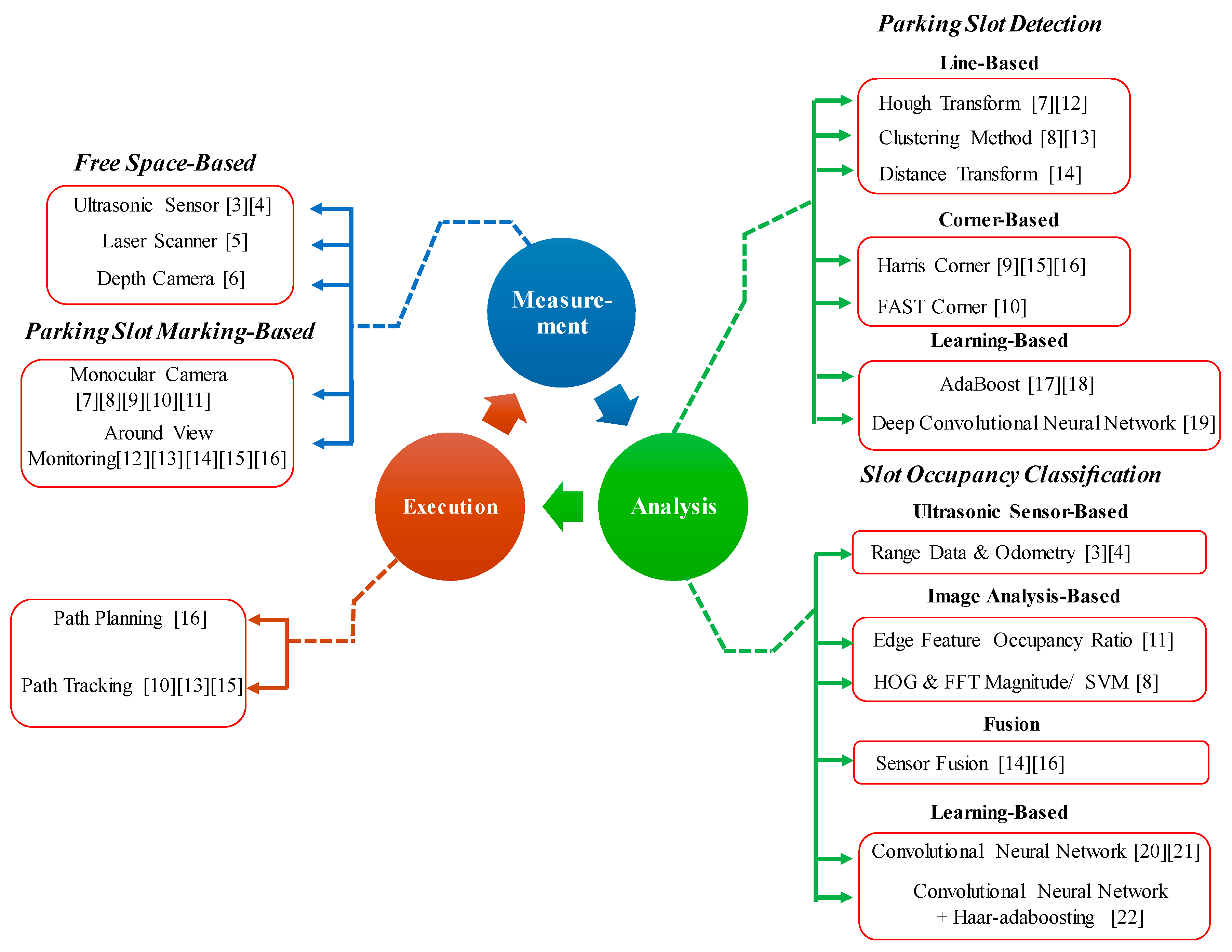
2. Literature Review
2.1. The Measurement Stage
2.1.1. Free Space-Based Sensors
2.1.2. Parking Space Marking-Based Sensors
2.2. The Analysis Stage
2.2.1. Parking Space Detection-Based Technology
2.2.2. Space Occupancy Classification-Based Technology
2.3. The Execution Stage
2.4. Summary
3. Algorithm to Detect Vacant Parking Spaces
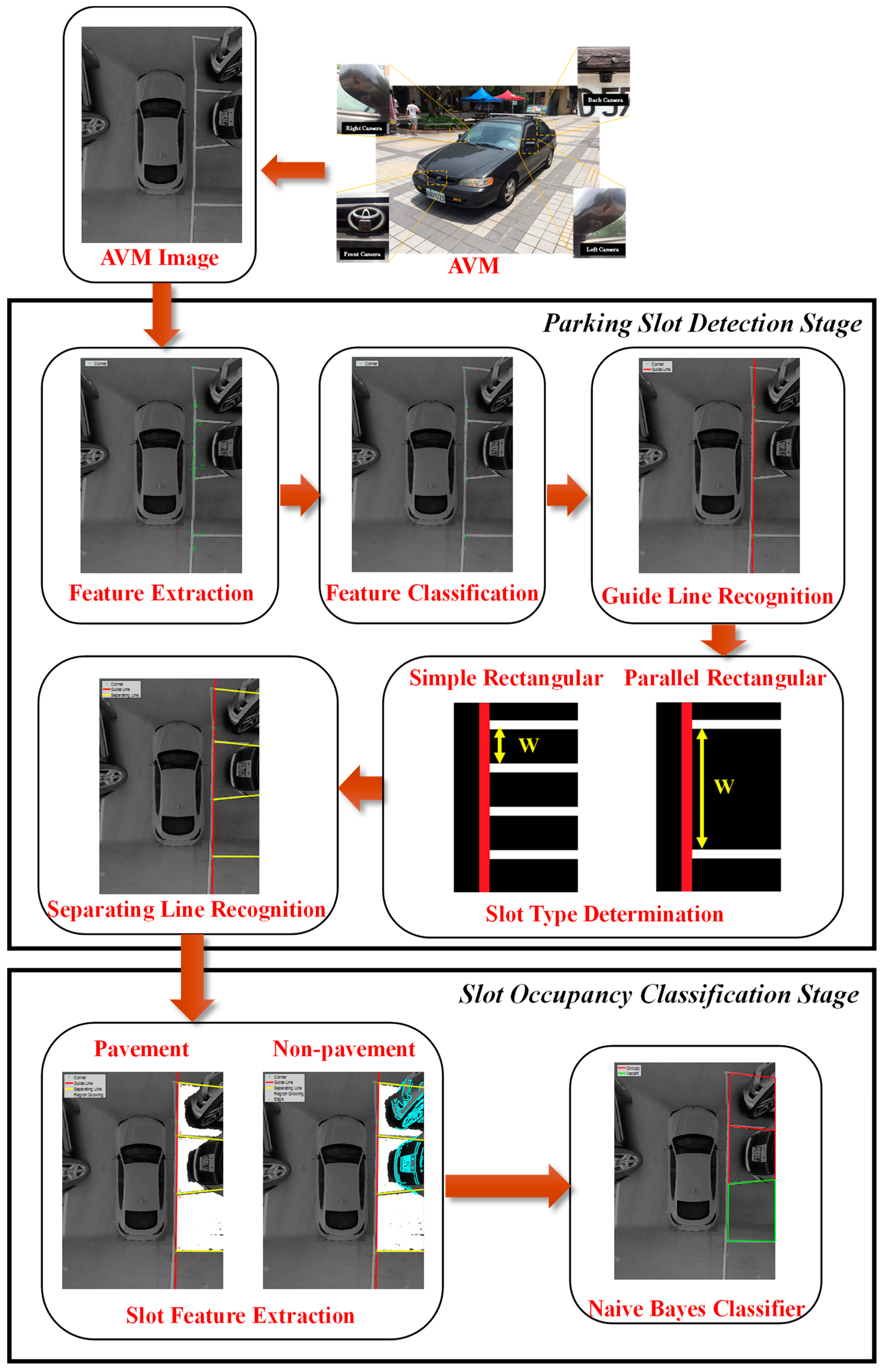
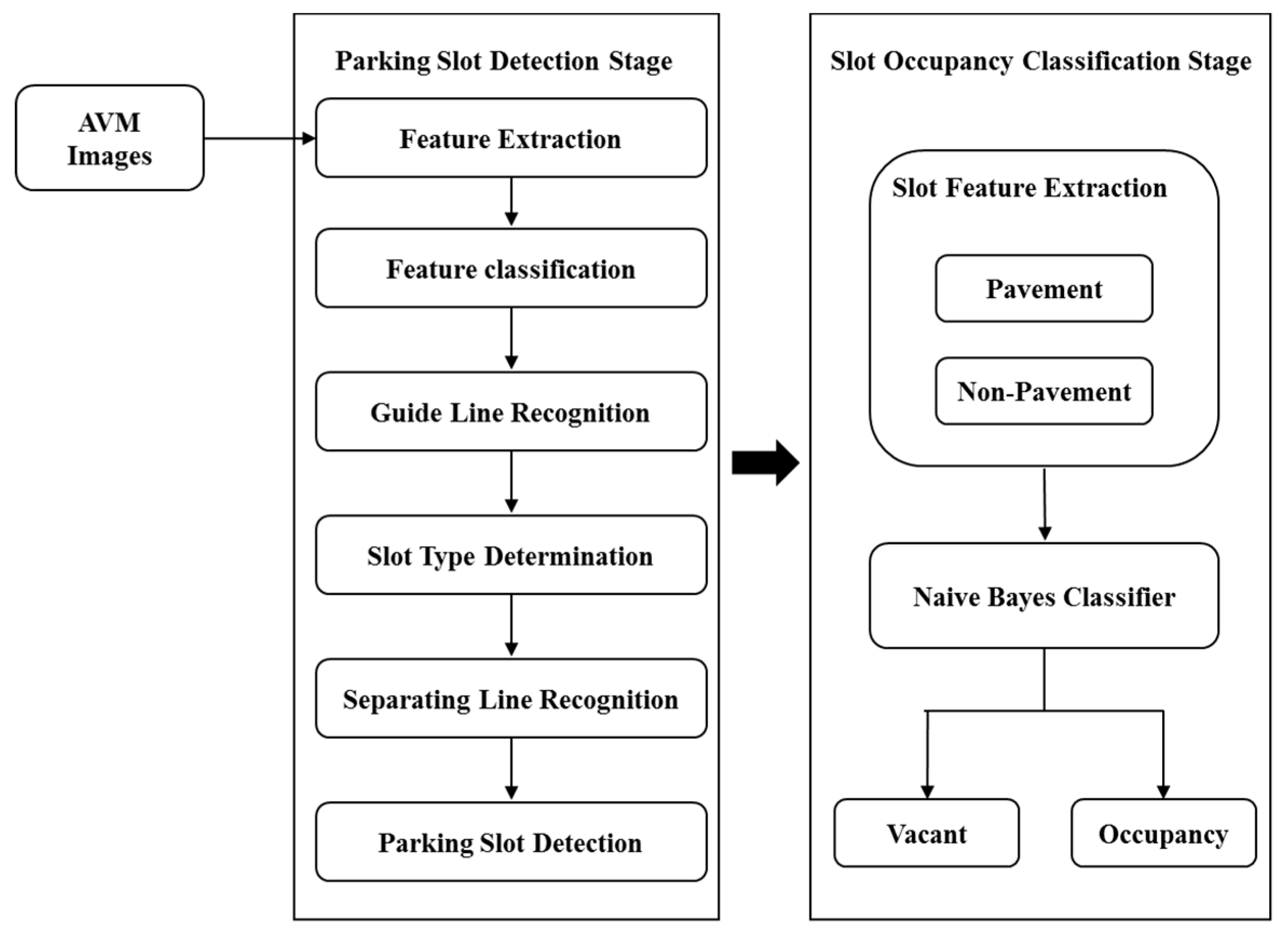
3.1. Algorithm Flowchart and Framework
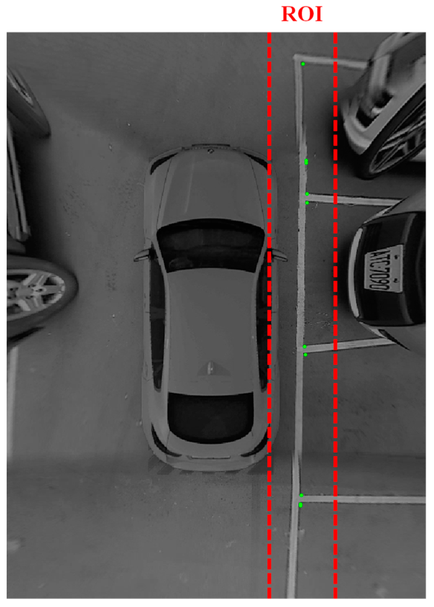
3.2. Parking Space Detection Stage
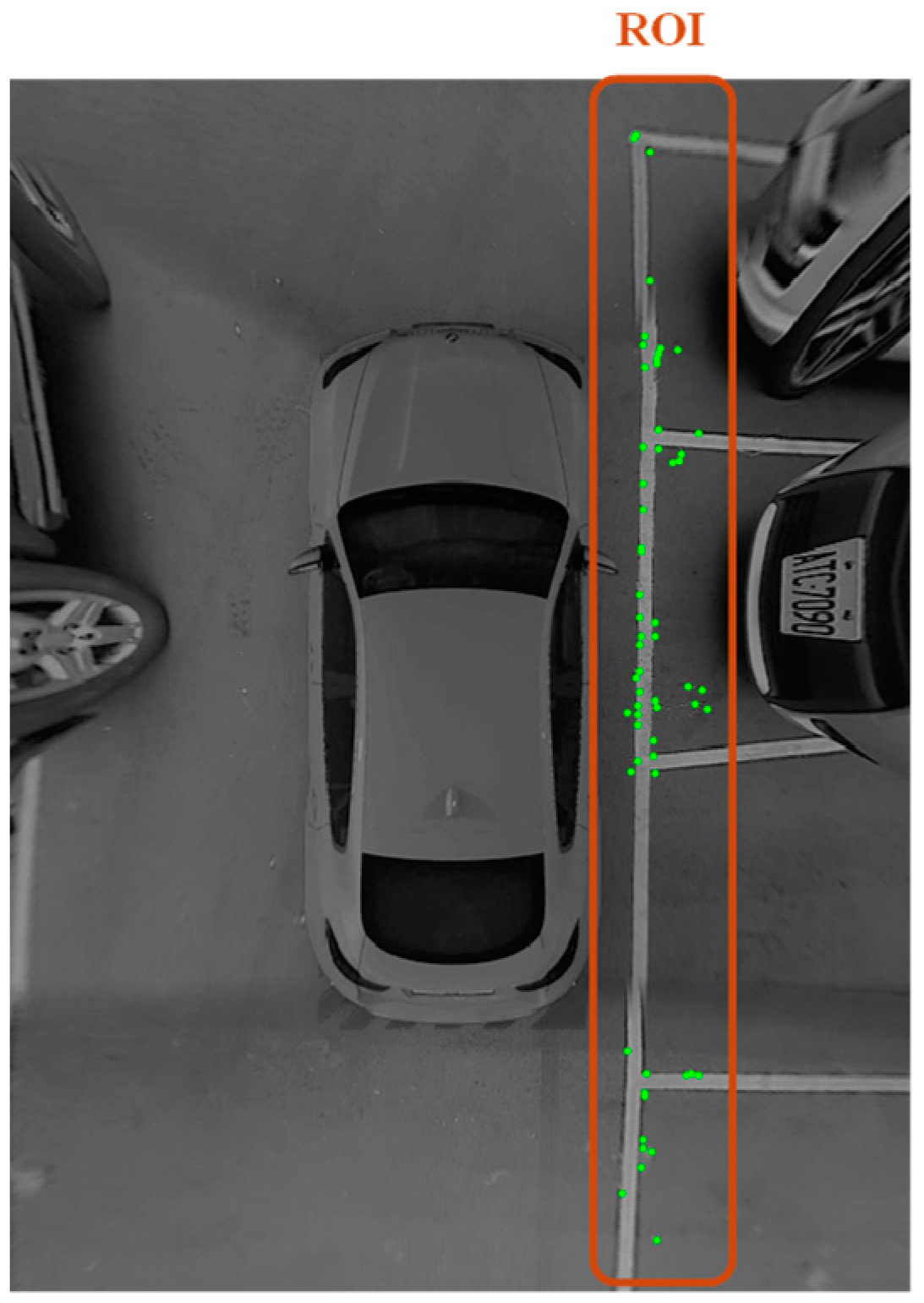
3.2.1. Feature Extraction
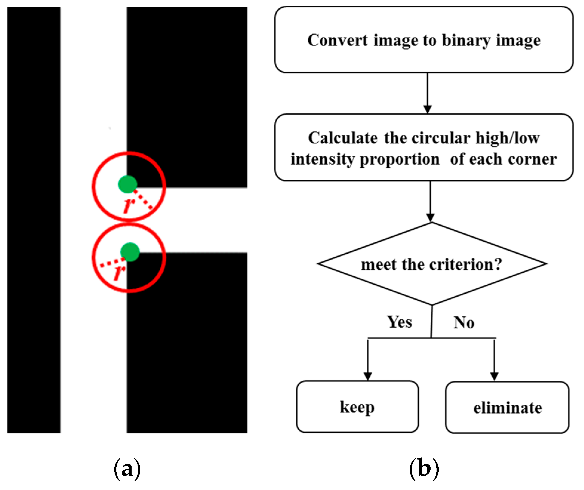
3.2.2. Feature Classification
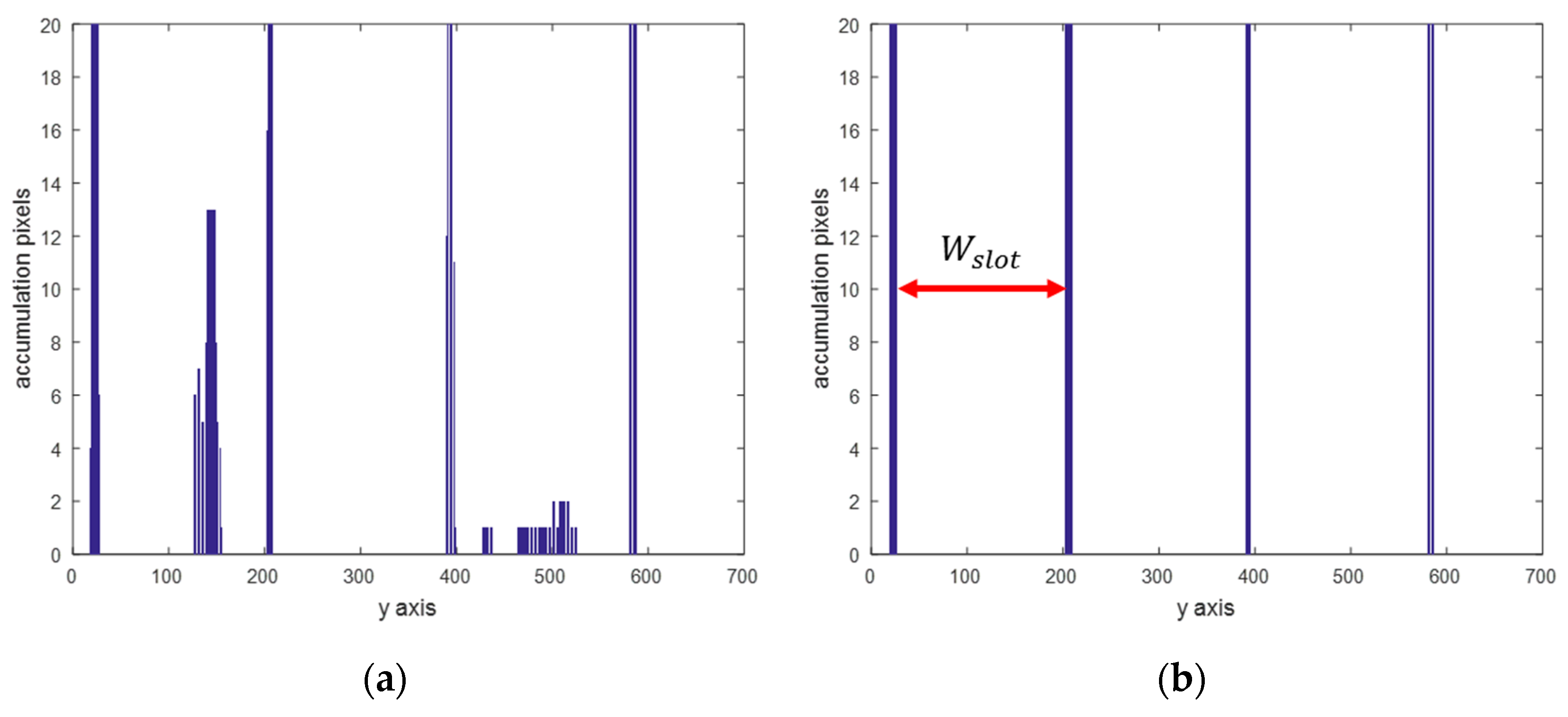
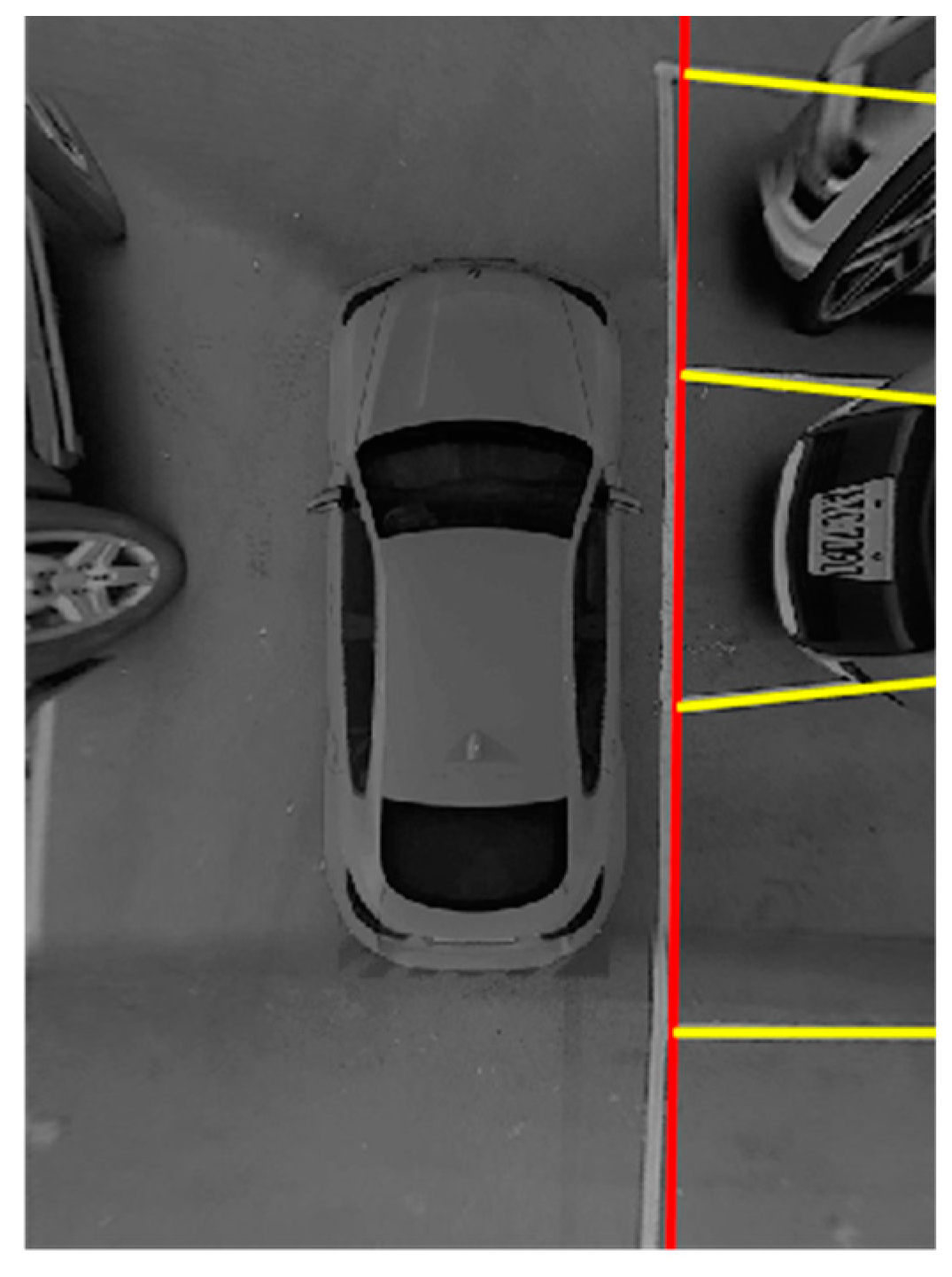
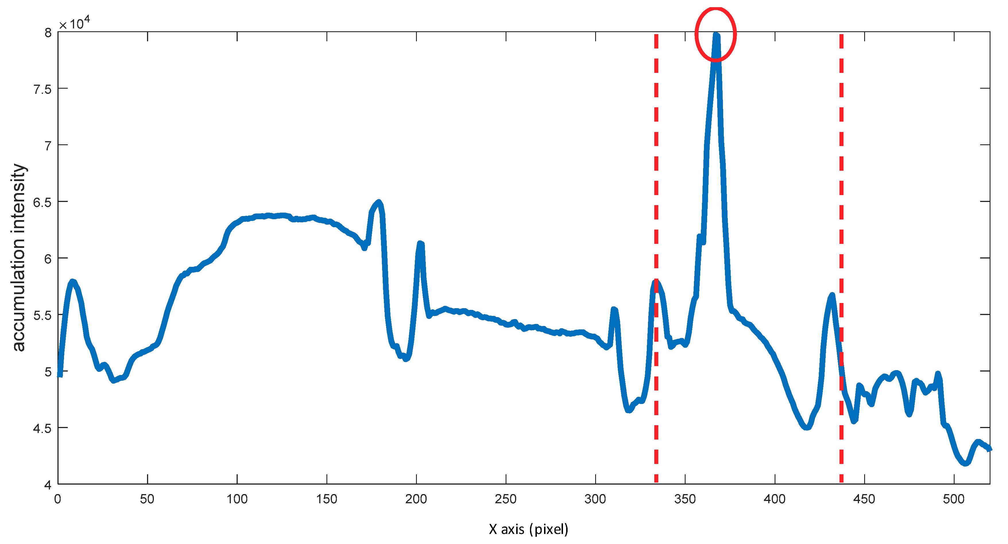
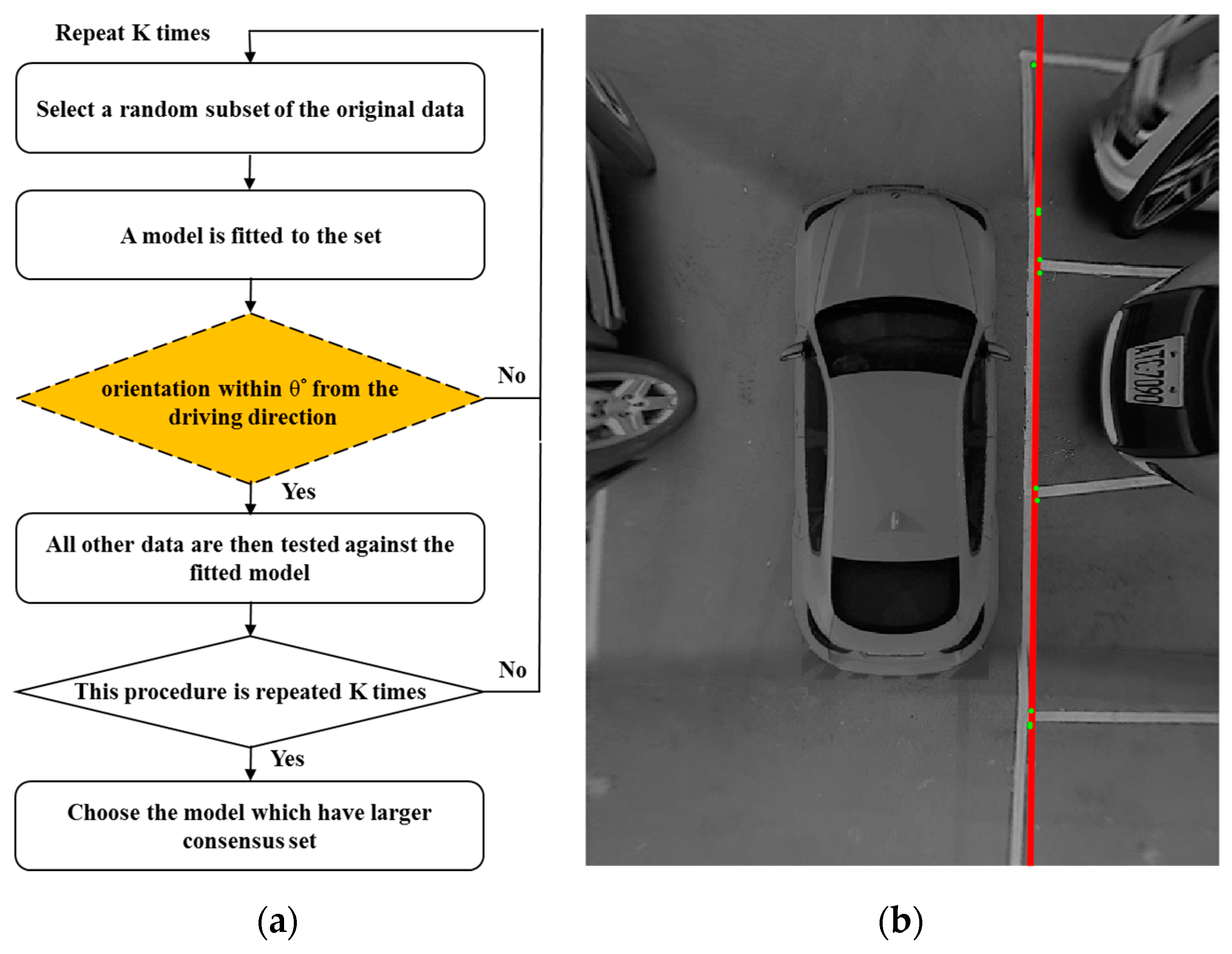
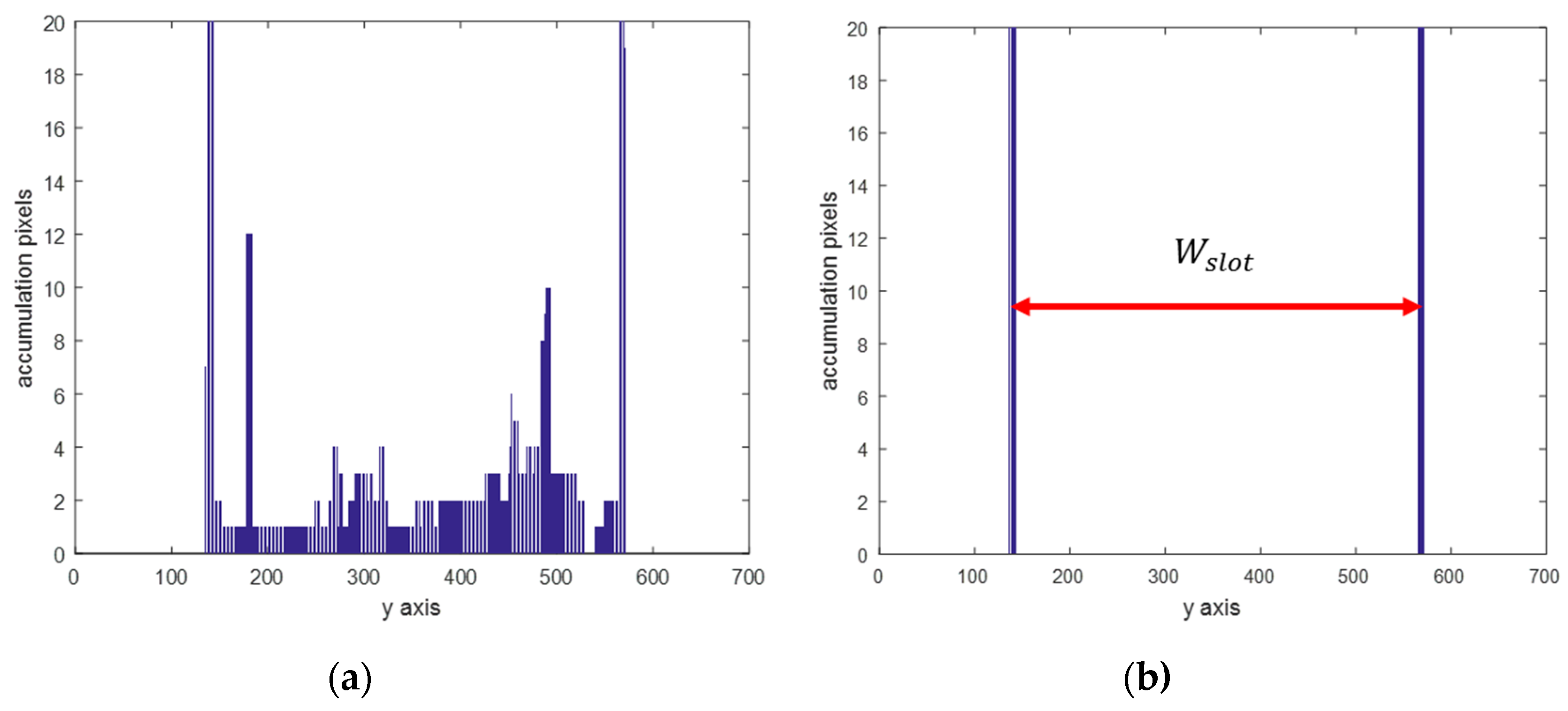
3.2.3. Lane Boundary Line Recognition
3.2.4. Space Type Determination
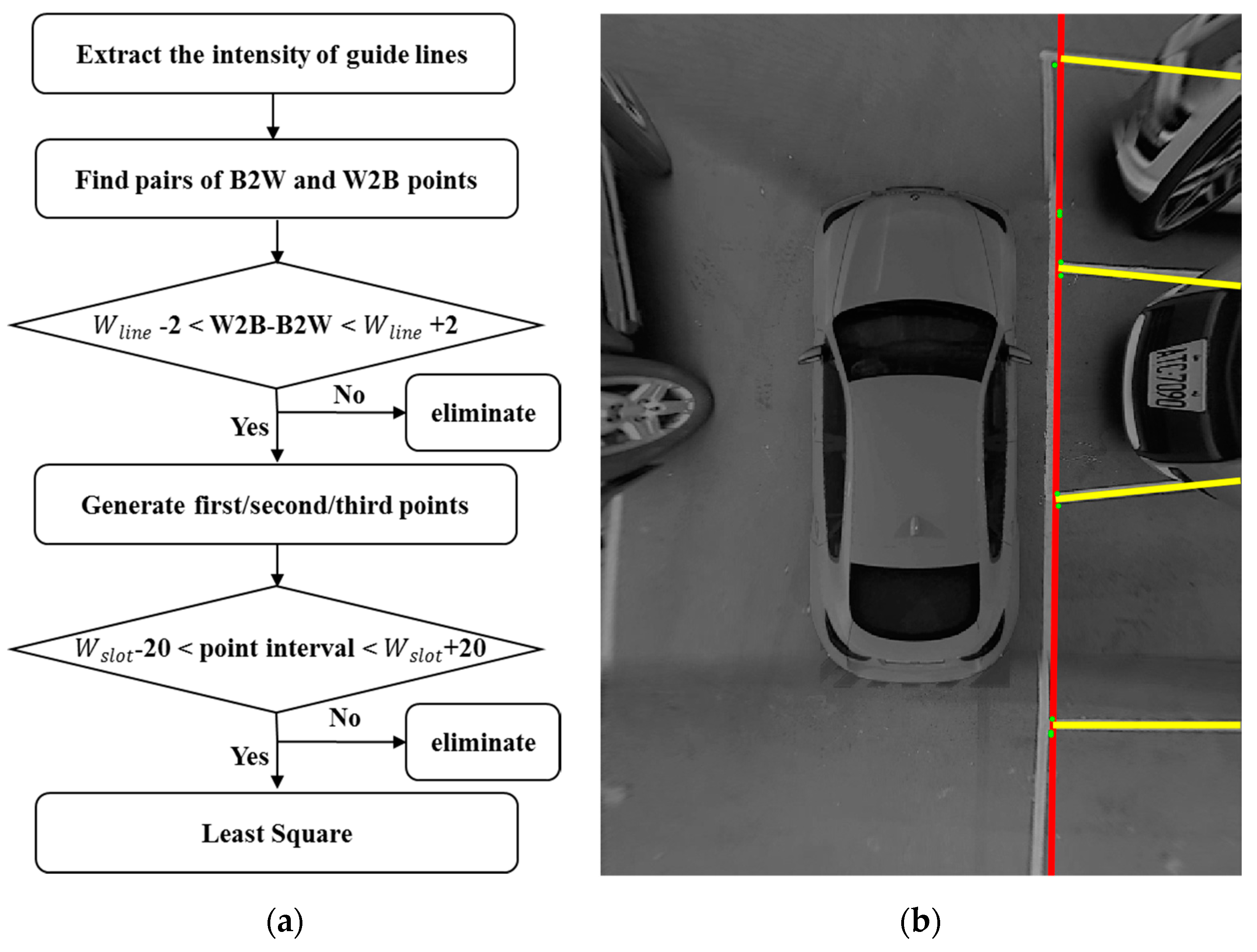
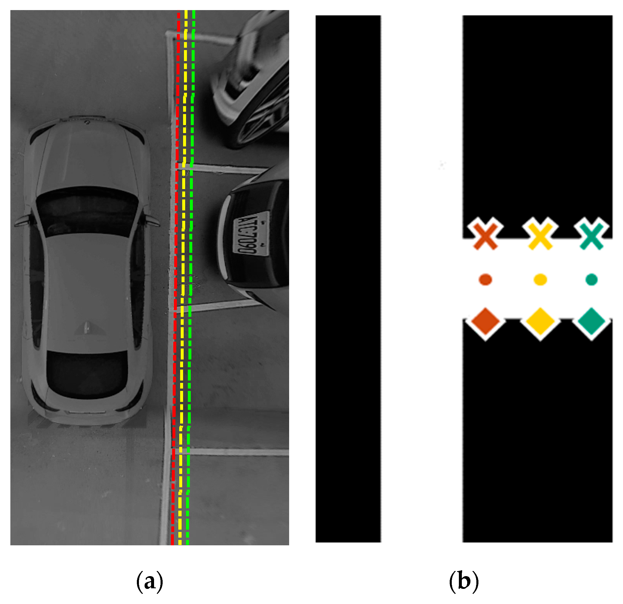
3.2.5. Divider Line Recognition
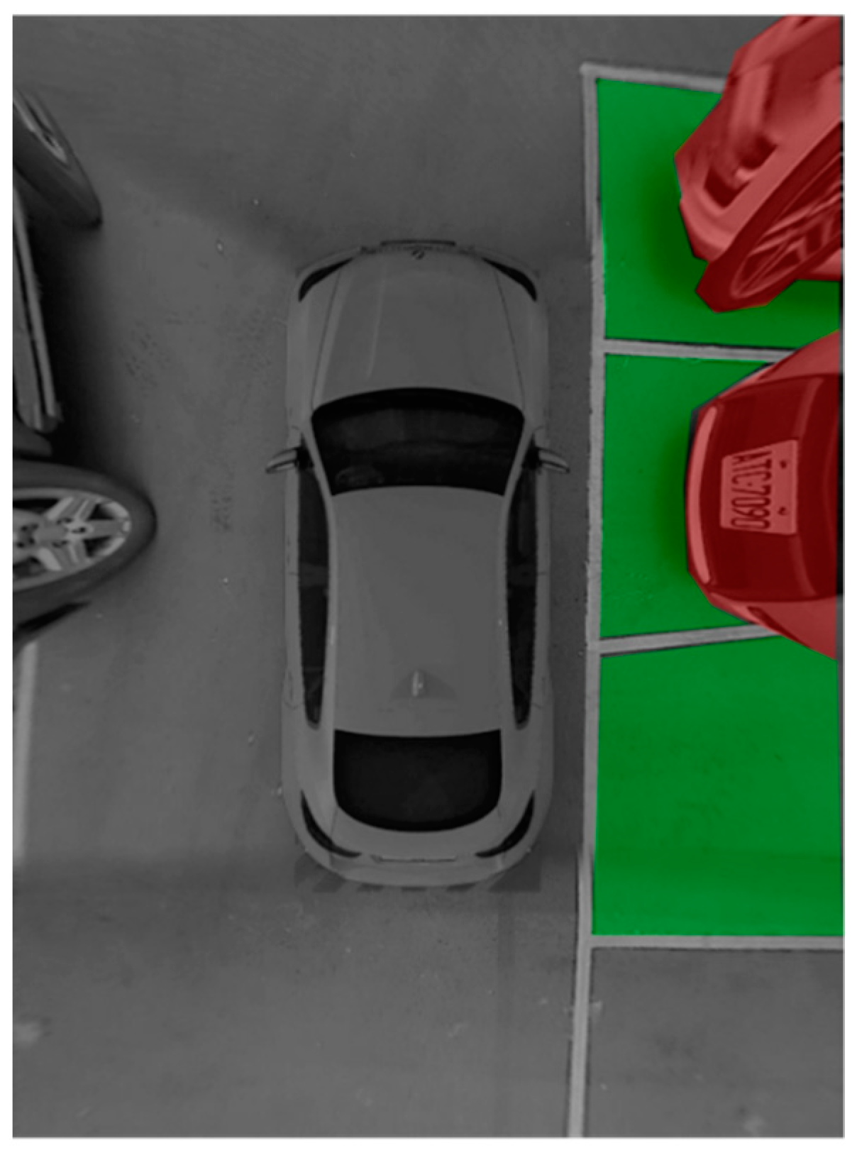
3.3. Space Occupancy Classification Stage
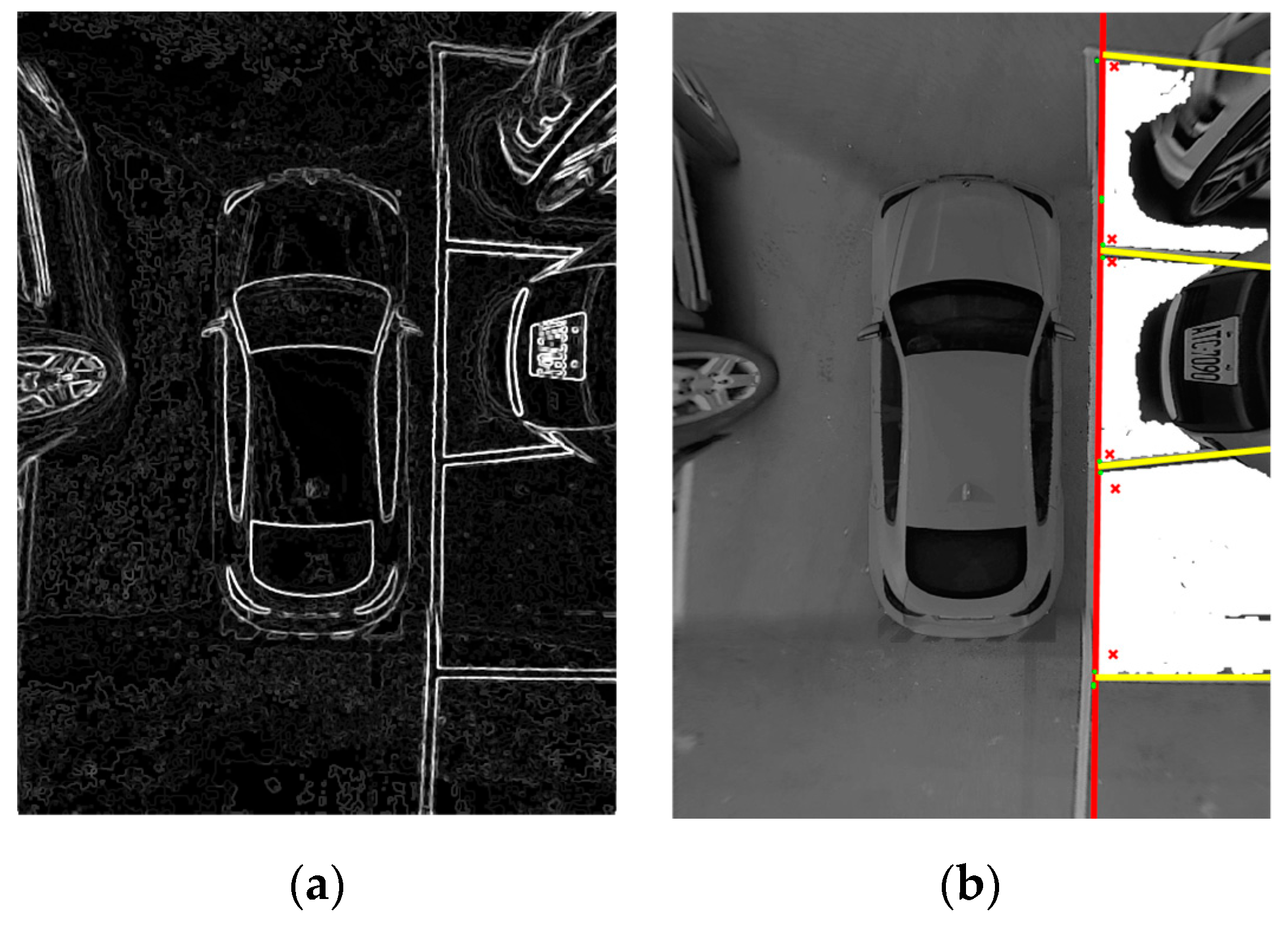
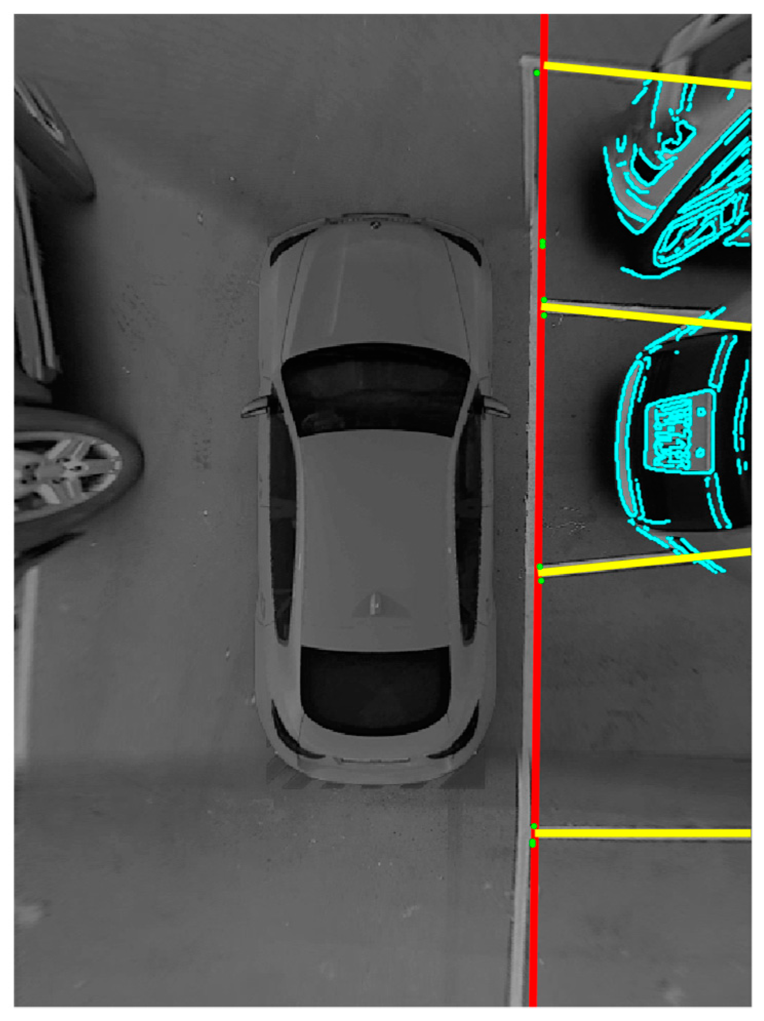
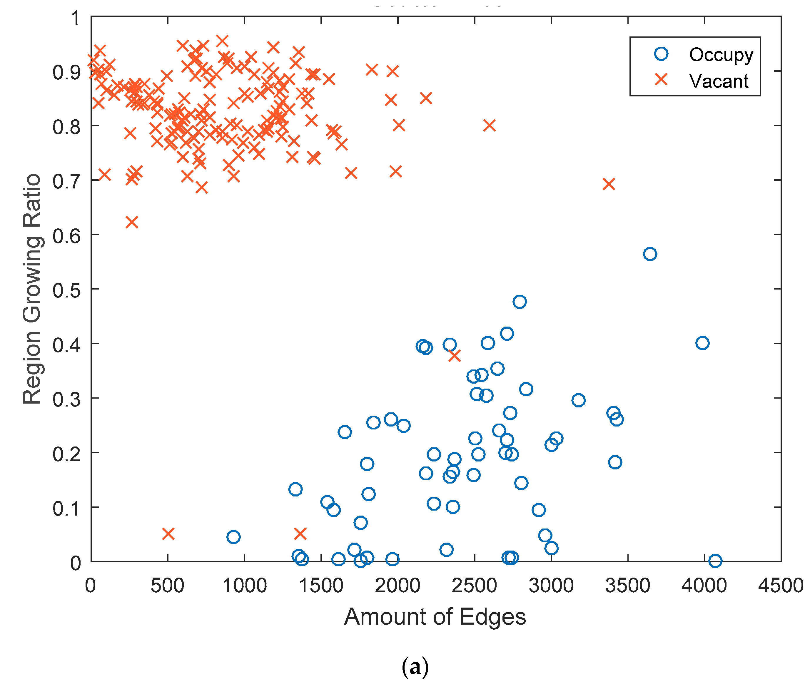
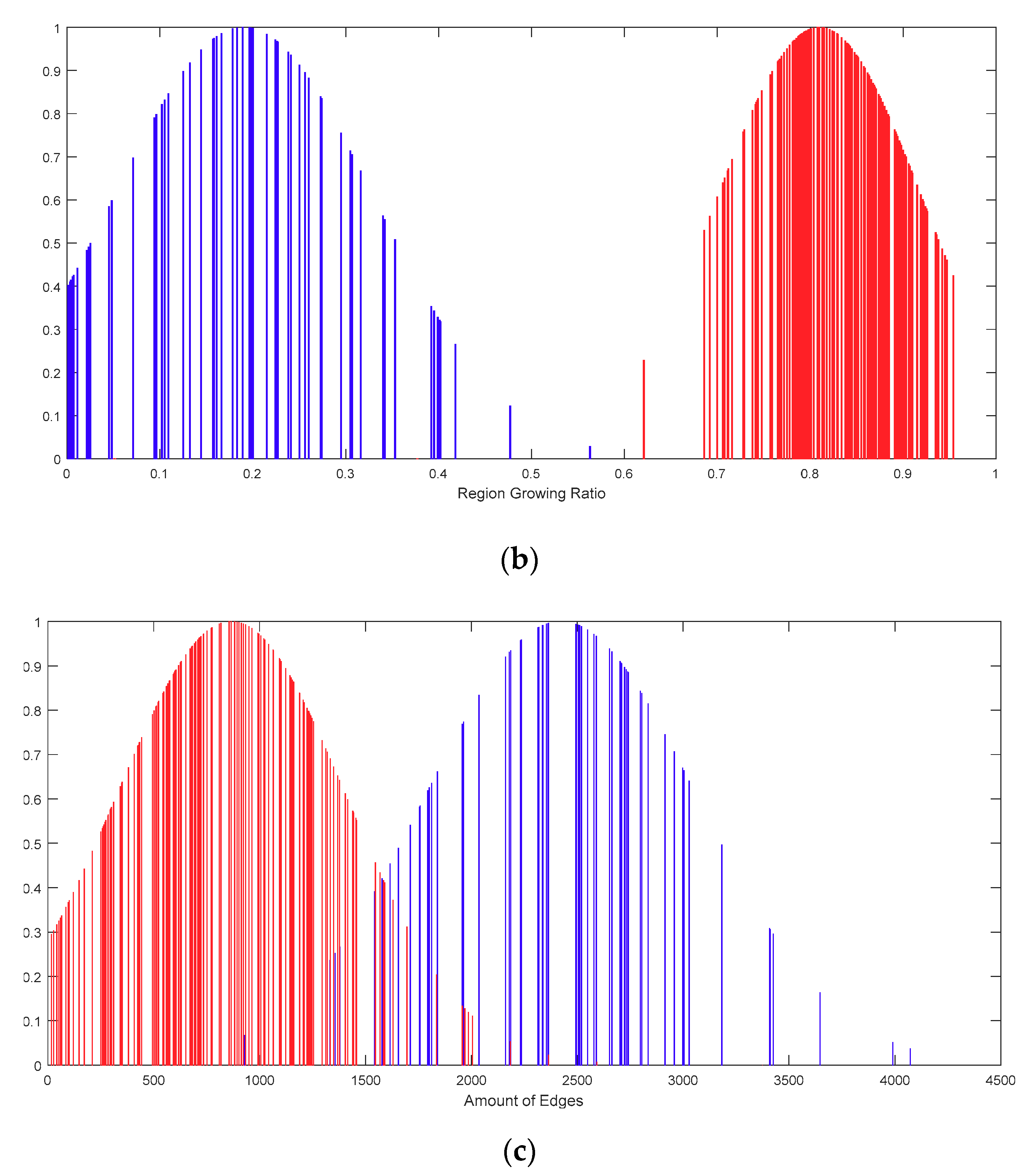
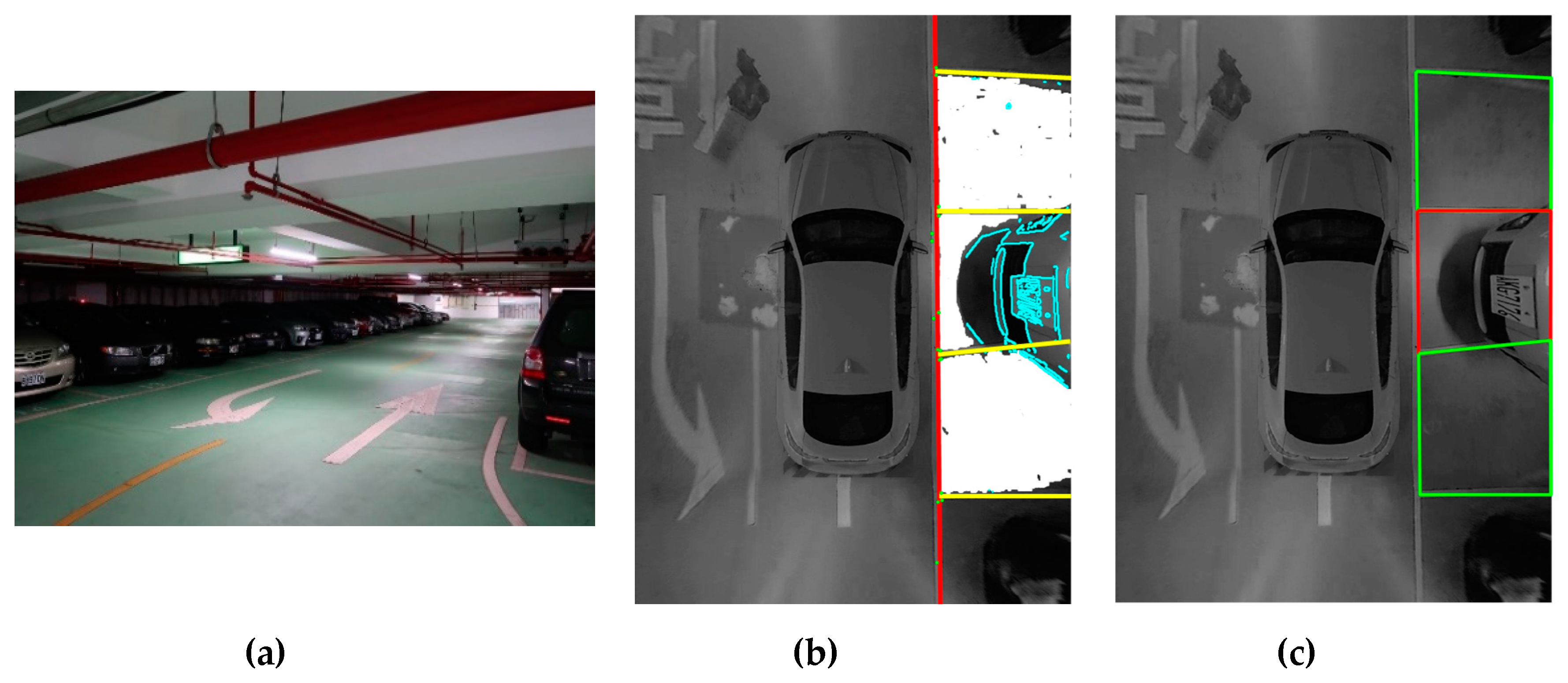
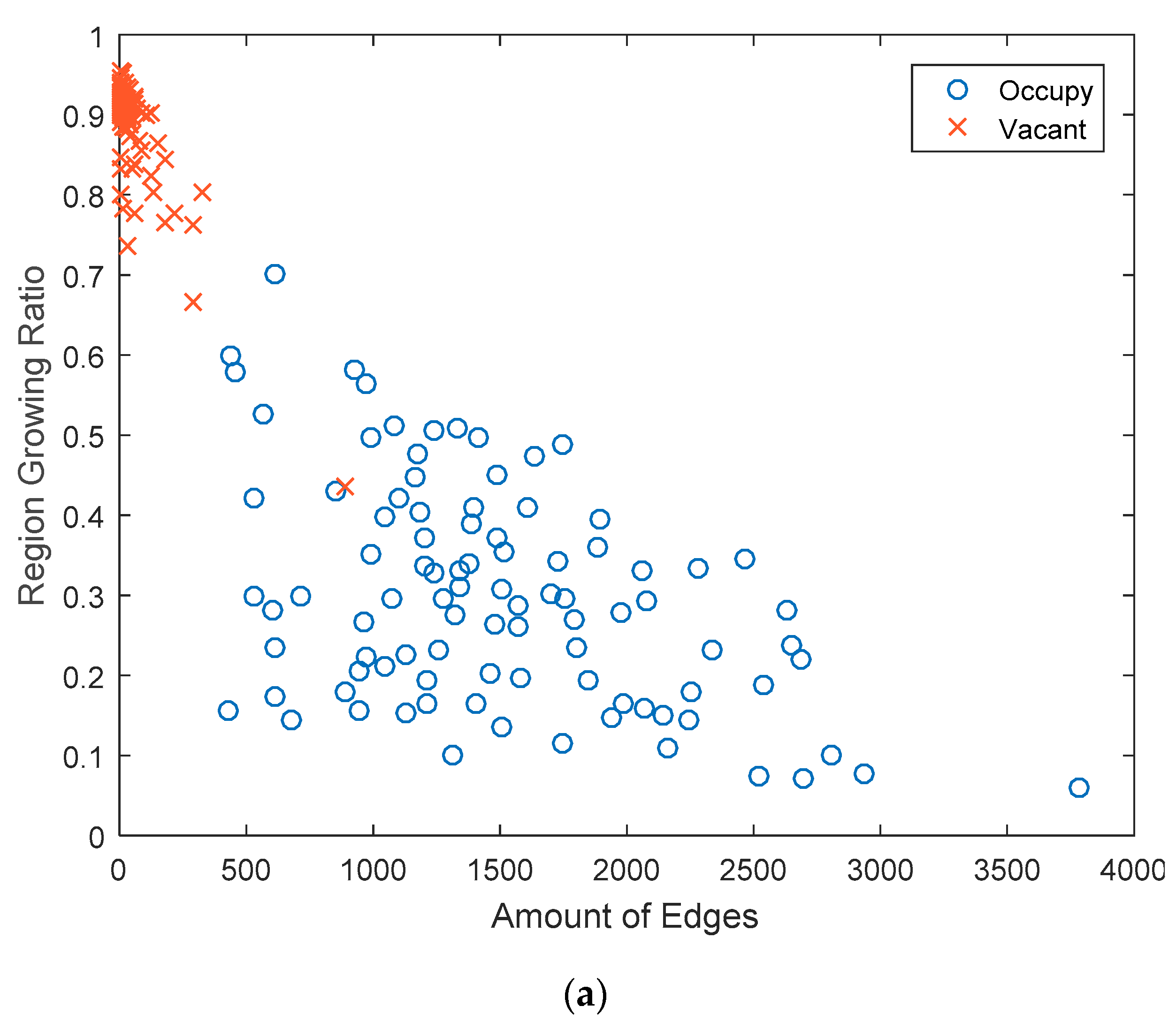
3.3.1. Parking Space Feature Extraction
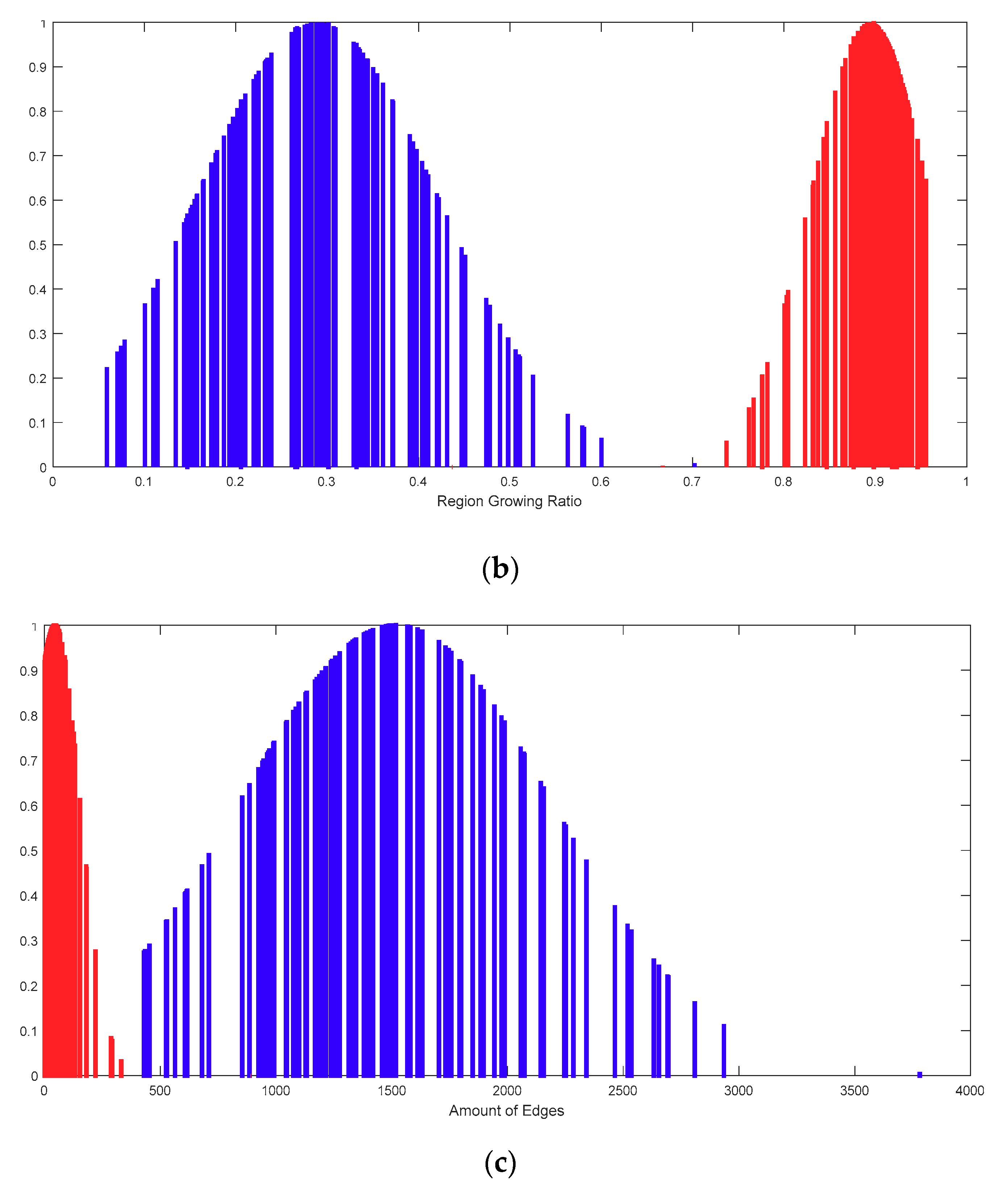
3.3.2. Naïve Bayes Classifier
4. Experimental Results
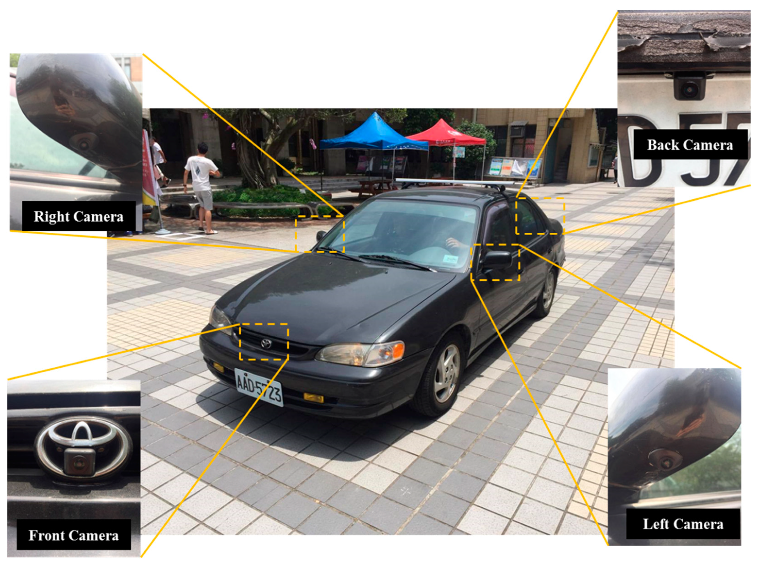
4.1. Experimental Equipment
4.2. Experimental Process
4.3. Experimental Results
4.3.1. Indoor Experimental Results
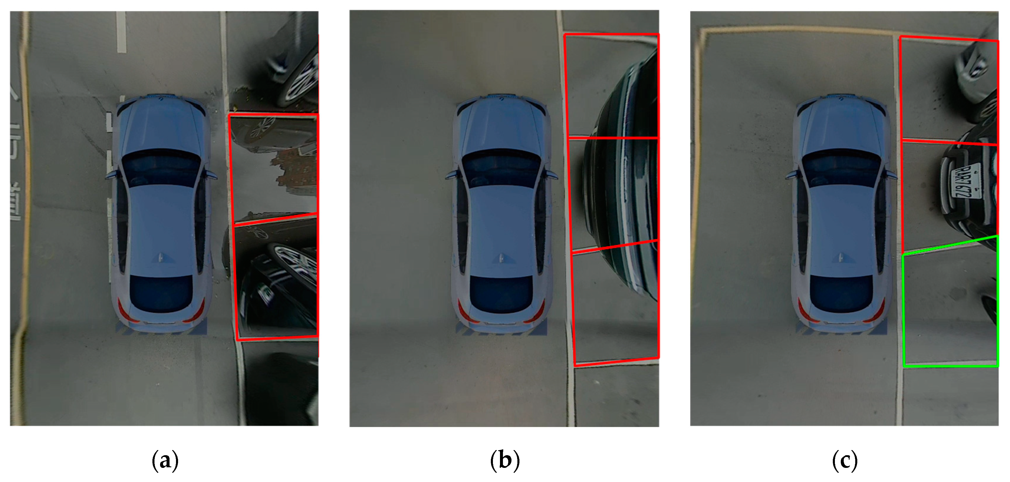
4.3.2. Outdoor Experimental Results
4.4. Performance Evaluation
- True positive (TP): Classified as occupied, and is actually occupied.
- False positive (FP): Classified as occupied, but is actually vacant.
- True negative (TN): Classified as vacant, and is actually vacant.
- False negative (FN): Classified as vacant, but is actually occupied.
4.4.1. Parking Space Detection Rates
4.4.2. Space Occupancy Classification Rates
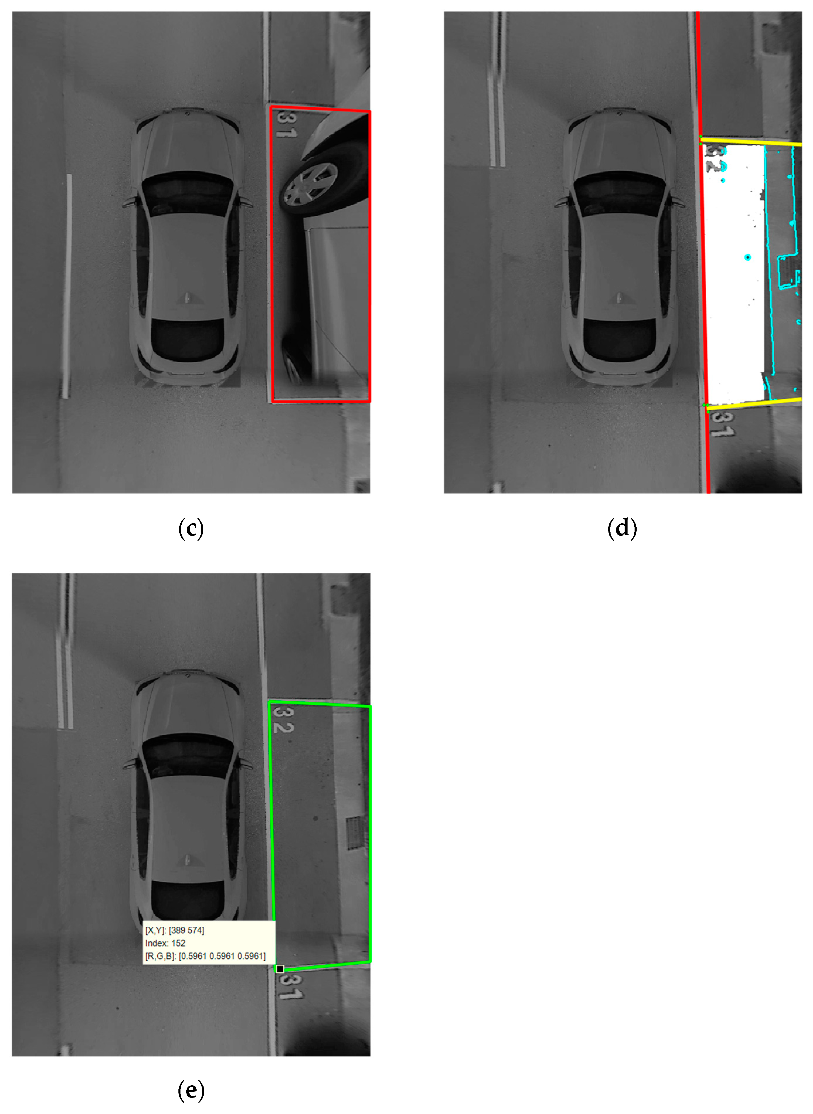
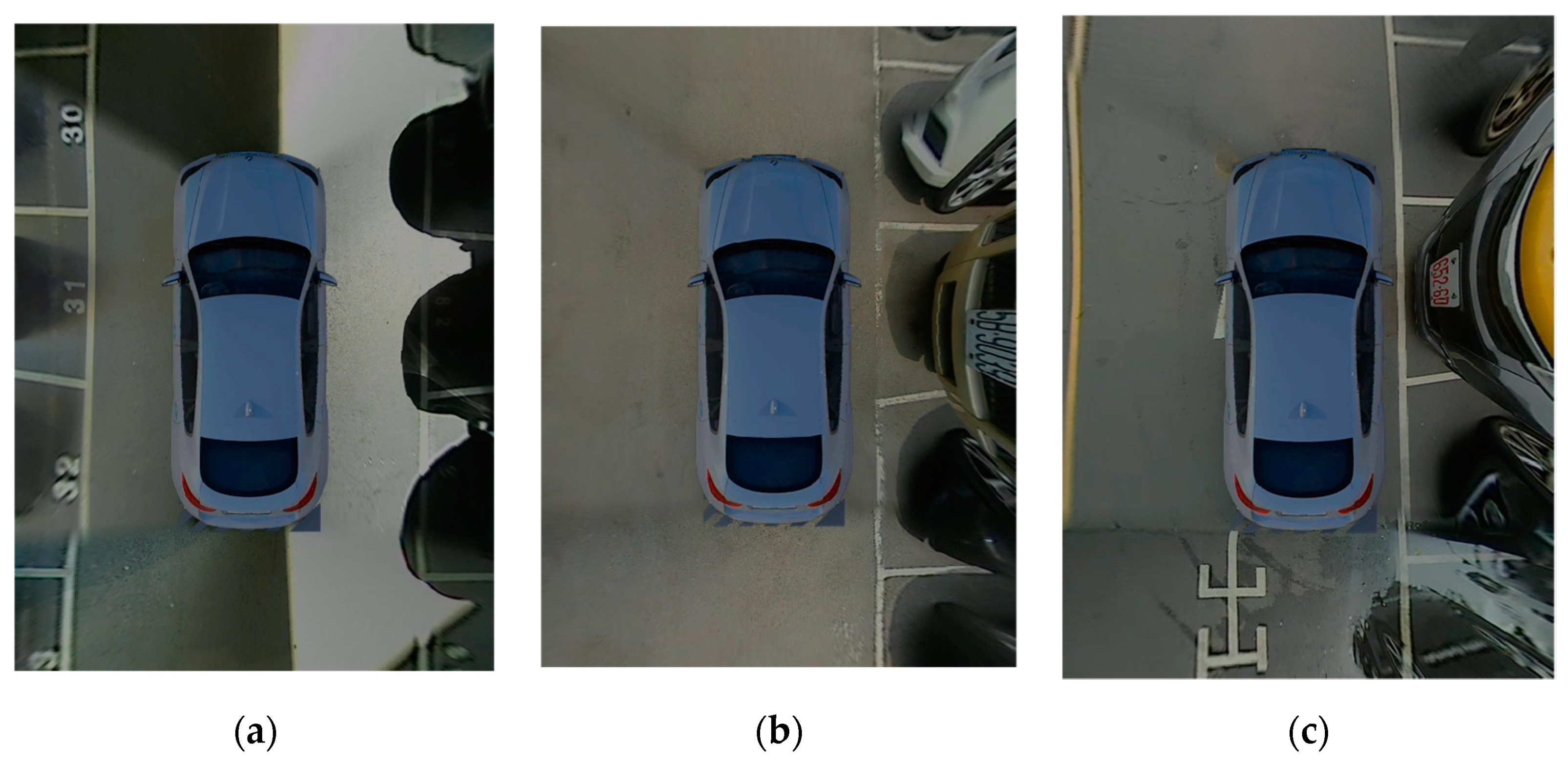
4.5. Analysis of Detection Failures
4.5.1. Parking Space Detection Failures
4.5.2. Space Occupancy Classification Failures
4.6. Summary
5. Conclusions and Prospects
Author Contributions
Funding
Conflicts of Interest
References
- Groh, B.H.; Friedl, M.; Linarth, A.G.; Angelopoulou, E. Advanced real-time indoor parking localization based on semi-static objects. In Proceedings of the 2014 17th International Conference on Information Fusion (FUSION), Salamanca, Spain, 7–10 July 2014; pp. 1–7. [Google Scholar]
- Ata, K.M.; Soh, A.C.; Ishak, A.J.; Jaafar, H.; Khairuddin, N.A. Smart Indoor Parking System Based on Dijkstra’s Algorithm. IJEEAS 2019, 2, 13–20. [Google Scholar]
- Jeong, S.H.; Choi, C.G.; Oh, J.N.; Yoon, P.J.; Kim, B.S.; Kim, M.; Lee, K.H. Low cost design of parallel parking assist system based on an ultrasonic sensor. Int. J. Autom. Technol. 2010, 11, 409–416. [Google Scholar] [CrossRef]
- Pohl, J.; Sethsson, M.; Degerman, P.; Larsson, J. A semi-automated parallel parking system for passenger cars. Proc. Inst. Mech. Eng. D J. Automob. Eng. 2006, 220, 53–65. [Google Scholar] [CrossRef]
- Jung, H.G.; Cho, Y.H.; Yoon, P.J.; Kim, J. Scanning laser radar-based target position designation for parking aid system. IEEE Trans. Intell. Transp. Syst. 2008, 9, 406–424. [Google Scholar] [CrossRef]
- Suhr, J.K.; Jung, H.G.; Bae, K.; Kim, J. Automatic free parking space detection by using motion stereo-based 3D reconstruction. Mach. Vis. Appl. 2010, 21, 163–176. [Google Scholar] [CrossRef]
- Jung, H.G.; Kim, D.S.; Yoon, P.J.; Kim, J. Parking slot markings recognition for automatic parking assist system. In Proceedings of the IEEE Intelligent Vehicles Symposium, Tokyo, Japan, 13–15 June 2006; pp. 106–113. [Google Scholar]
- Lee, S.; Seo, S.W. Available parking slot recognition based on slot context analysis. IET Intell. Transp. Syst. 2016, 10, 594–604. [Google Scholar] [CrossRef]
- Suhr, J.K.; Jung, H.G. Full-automatic recognition of various parking slot markings using a hierarchical tree structure. Opt. Eng. 2013, 52, 037203. [Google Scholar] [CrossRef]
- Sevillano, X.; Màrmol, E.; Fernandez-Arguedas, V. Towards smart traffic management systems: Vacant on-street parking spot detection based on video analytics. In Proceedings of the 17th International Conference on Information Fusion, Salamanca, Spain, 7–10 July 2014. [Google Scholar]
- Wang, C.; Zhang, H.; Yang, M.; Wang, X.; Ye, L.; Guo, C. Automatic parking based on a bird’s eye view vision system. Adv. Mech. Eng. 2014, 2014, 847406. [Google Scholar] [CrossRef]
- Hamada, K.; Hu, Z.; Fan, M.; Chen, H. Surround view based parking lot detection and tracking. In Proceedings of the IEEE Intelligent Vehicles Symposium, Seoul, Korea, 28 June–1 July 2015; pp. 1106–1111. [Google Scholar]
- Lee, S.; Hyeon, D.; Park, G.; Baek, I.J.; Kim, S.W.; Seo, S.W. Directional-DBSCAN: Parking-slot Detection using a Clustering Method in Around-View Monitoring System. In Proceedings of the IEEE Intelligent Vehicles Symposium, Gothenburg, Sweden, 19–22 June 2016; pp. 349–354. [Google Scholar]
- Suhr, J.K.; Jung, H.G. Automatic Parking Space Detection and Tracking for Underground and Indoor Environments. IEEE Trans. Ind. Electr. 2016, 63, 5687–5698. [Google Scholar] [CrossRef]
- Suhr, J.K.; Jung, H.G. Fully-automatic recognition of various parking slot markings in Around View Monitor (AVM) image sequences. In Proceedings of the 2012 15th International IEEE Conference on Intelligent Transportation Systems, Anchorage, AK, USA, 16–19 September 2012; pp. 1294–1299. [Google Scholar]
- Suhr, J.K.; Jung, H.G. Sensor fusion-based vacant parking slot detection and tracking. Trans. Intell. Transp. Syst. 2014, 15, 21–36. [Google Scholar] [CrossRef]
- Zhang, L.; Li, X.; Huang, J.; Shen, Y.; Wang, D. Vision-Based Parking-Slot Detection: A Benchmark and A Learning-Based Approach. Symmetry 2018, 10, 64. [Google Scholar] [CrossRef]
- Li, L.; Zhang, L.; Li, X.; Liu, X.; Shen, Y.; Xiong, L. Vision-based parking-slot detection: A benchmark and a learning-based approach. In Proceedings of the 2017 IEEE International Conference on Multimedia and Expo, Hong Kong, China, 10–14 July 2017; pp. 649–654. [Google Scholar]
- Zhang, L.; Huang, J.; Li, X.; Xiong, L. Vision-Based Parking-Slot Detection: A DCNN-Based Approach and a Large-Scale Benchmark Dataset. IEEE Trans. Image Process. 2018, 27, 5350–5364. [Google Scholar] [CrossRef] [PubMed]
- Amato, G.; Carrara, F.; Falchi, F.; Gennaro, C.; Vairo, C. Car parking occupancy detection using smart camera networks and deep learning. In Proceedings of the 2016 IEEE Symposium on Computers and Communication (ISCC), Messina, Italy, 27–30 June 2016; pp. 1212–1217. [Google Scholar]
- Amato, G.; Carrara, F.; Falchi, F.; Gennaro, C.; Meghini, C.; Vairo, C. Deep learning for decentralized parking lot occupancy detection. Expert Syst. Appl. 2017, 72, 327–334. [Google Scholar] [CrossRef]
- Xiang, X.; Lv, N.; Zhai, M.; Saddik, A.E. Real-time parking occupancy detection for gas stations based on haar-adaboosting and cnn. IEEE Sens. J. 2017, 17, 6360–6367. [Google Scholar] [CrossRef]
- Lin, C.F.; Hsu, C.W.; Ko, M.K.; Yao, C.C.; Chang, K.J. A Multiple Turn Achievement of Advanced Parking Guidance System in Parallel Parking via Sensor Fusion. In International Symposium on Advanced Vehicle Control; Automotive Research & Testing Center: Changhua, Taiwan, 2010. [Google Scholar]
- Rosten, E.; Drummond, T. Machine learning for high speed corner detection. In Proceedings of the 9th Euproean Conference on Computer Vision, Graz, Austria, 7–13 May 2006; pp. 430–443. [Google Scholar]
- Fischler, M.A.; Bolles, R.C. Random sample consensus: A paradigm for model fitting with applications to image analysis and automated cartography. Commun. ACM 1981, 24, 381–395. [Google Scholar] [CrossRef]
- Marquardt, D. An Algorithm for Least-squares Estimation of Nonlinear Parameters. SIAM J. Appl. Math. 1963, 11, 431–441. [Google Scholar] [CrossRef]
- Canny, J. A computational approach to edge detection. IEEE Trans. Pattern Anal. Mach. Intell. 1986, 8, 679–698. [Google Scholar] [CrossRef] [PubMed]
- Thrun, S.; Burgard, W.; Fox, D. Probabilistic Robotics; MIT Press: Cambridge, MA, USA, 2005. [Google Scholar]
- Nissan Owner Channel: 2018 Nissan Kicks—Intelligent Around View Monitor (I-AVM). Available online: https://www.youtube.com/watch?v=n1zgKVLD9OA (accessed on 25 July 2019).


| Header | Growing Ratio | Edges (Pixels) | Status |
|---|---|---|---|
| First slot | 0.894 | 44 | Vacant |
| Second slot | 0.199 | 1556 | Occupied |
| Third slot | 0.845 | 230 | Vacant |
| Header | Growing Ratio | Edges (Pixels) | Status |
|---|---|---|---|
| First slot | 0.394 | 1654 | Occupied |
| Second slot | 0.908 | 0 | Vacant |
| Third slot | 0.325 | 1325 | Occupied |
| Header | Growing Ratio | Edges (Pixels) | Status |
|---|---|---|---|
| First slot | 0.473 | 696 | Occupied |
| Second slot | 0.744 | 5 | Vacant |
| Third slot | 0.339 | 480 | Occupied |
| Header | Growing Ratio | Edges (Pixels) | Status |
|---|---|---|---|
| First slot | 0.25 | 2036 | Occupied |
| Second slot | 0.928 | 867 | Vacant |
| Scene | Indoor | Outdoor | ||
|---|---|---|---|---|
| Computing time (s) | 0.17 | 0.16 | ||
| Parking type | Perpendicular parking | Perpendicular parking | Parallel Parking | Total |
| # of existing slots | 311 | 545 | 233 | 778 |
| # of detected slots | 274 | 521 | 224 | 745 |
| # of correctly slots | 263 | 519 | 224 | 743 |
| Recall (%) | 84.6 | 95.2 | 96.1 | 95.5 |
| Precision (%) | 96 | 99.6 | 100 | 99.7 |
| Scene | Indoor | Outdoor | ||||
|---|---|---|---|---|---|---|
| Feature type | Edge-based [10] | Growing -based | Fusion | Edge-based [10] | Growing -based | Fusion |
| Computing time (s) | 0.14 | 0.13 | 0.27 | 0.13 | 0.1 | 0.24 |
| # of occupied slots (positive) | 175 | 173 | 179 | 394 | 333 | 333 |
| # of vacant slots (negative) | 88 | 90 | 84 | 349 | 410 | 410 |
| # of false negative | 17 | 21 | 12 | 6 | 11 | 7 |
| # of false positive | 4 | 6 | 3 | 77 | 20 | 18 |
| FNR (%) | 9.7 | 12.1 | 6.7 | 1.5 | 3.3% | 2.1 |
| FPR (%) | 4.5 | 6.7 | 3.6 | 22 | 4.9 | 4.4 |
| Error Rate (%) | 7.1 | 9.4 | 5.2 | 11.8 | 4.1 | 3.3 |
© 2019 by the authors. Licensee MDPI, Basel, Switzerland. This article is an open access article distributed under the terms and conditions of the Creative Commons Attribution (CC BY) license (http://creativecommons.org/licenses/by/4.0/).
Share and Cite
Hsu, C.-M.; Chen, J.-Y. Around View Monitoring-Based Vacant Parking Space Detection and Analysis. Appl. Sci. 2019, 9, 3403. https://doi.org/10.3390/app9163403
Hsu C-M, Chen J-Y. Around View Monitoring-Based Vacant Parking Space Detection and Analysis. Applied Sciences. 2019; 9(16):3403. https://doi.org/10.3390/app9163403
Chicago/Turabian StyleHsu, Chih-Ming, and Jian-Yu Chen. 2019. "Around View Monitoring-Based Vacant Parking Space Detection and Analysis" Applied Sciences 9, no. 16: 3403. https://doi.org/10.3390/app9163403
APA StyleHsu, C.-M., & Chen, J.-Y. (2019). Around View Monitoring-Based Vacant Parking Space Detection and Analysis. Applied Sciences, 9(16), 3403. https://doi.org/10.3390/app9163403