Improved Hierarchical Adaptive Deep Belief Network for Bearing Fault Diagnosis

Abstract

Rotating machinery plays a vital role in modern mechanical systems. Effective state monitoring of a rotary machine is important to guarantee its safe operation and prevent accidents. Traditional bearing fault diagnosis techniques rely on manual feature extraction, which in turn relies on complex signal processing and rich professional experience. The collected bearing signals are invariably complicated and unstable. Deep learning can voluntarily learn representative features without a large amount of prior knowledge, thus becoming a significant breakthrough in mechanical fault diagnosis. A new method for bearing fault diagnosis, called improved hierarchical adaptive deep belief network (DBN), which is optimized by Nesterov momentum (NM), is presented in this research. The frequency spectrum is used as inputs for feature learning. Then, a learning rate adjustment strategy is applied to adaptively select the descending step length during gradient updating, combined with NM. The developed method is validated by bearing vibration signals. In comparison to support vector machine and the conventional DBN, the raised approach exhibits a more satisfactory performance in bearing fault type and degree diagnosis. It can steadily and effectively improve convergence during model training and enhance the generalizability of DBN.

1. Introduction

Mechanical equipment failures in rotating machinery, such as aircraft engines, are usually caused by damage and malfunction of critical components. Although regular maintenance and forced retirement can improve the safety and reliability of equipment operation, these solutions result in a heavy economic burden and waste of resources. According to statistics, in rotating machinery that uses rolling bearings, approximately 40% of the mechanical failures are due to bearing damage [1]. Therefore, effective fault diagnosis of these key components can provide a strong basis for the evaluation of the operational status of mechanical equipment, thereby reducing maintenance costs [2]. The traditional methods based on signal processing mainly use related expertise to extract faulty components from initial noisy signals. Currently, signal processing methods based on time–frequency analysis have caught the attention of scholars, including empirical mode decomposition, wavelet packet transform, short-time Fourier transform, and so forth [3,4,5]. Wang et al. [6] diagnosed the rubbing fault by extending variational mode decomposition method. Wang et al. [7] combined independent component analysis with empirical model decomposition to separate the bearing fault components in wind turbine gearboxes. Wang et al. [8] used the square envelope analysis to study the performance degradation evaluation under Gaussian noise. Li et al. [9] advanced a strategy that combines intrinsic characteristic-scale decomposition and turntable Q-factor wavelet transform to detect the early bearing fault. Improved Local Mean Decomposition (LMD) can effectively diagnose bearing fault types by expanding the sides of the vibration signal to suppress edge effects [10]. Fault-related features have been revealed successfully in the aforementioned applications. However, satisfactory performance is achieved on the basis of professional knowledge, a requirement that is sometimes difficult for field maintenance personnel to meet.

On the basis of these considerations, the machine-learning-based approaches tailored for fault diagnosis, such as artificial neural network (ANN) [11], decision tree [12], and support vector machine (SVM) [13] have been gradually developed. The goal is to reduce human intervention as much as possible and move toward an intelligent direction. As a result, deep learning methods are proposed, inspired by the artificial intelligence and machine learning [14], which correspond to traditional shallow machine-learning methods. Since its introduction, deep learning has shown strong capabilities in speech recognition, image processing, and other fields. Especially, some classic networks such as deep belief network (DBN) [15] and convolutional neural network (CNN) [16] have been successfully ameliorated for fault detection. Qin et al. [17] presented a new model based on DBNs, with improved logistic sigmoid units for fault identification of wind turbine gearboxes. Zhang et al. [18] used CNN to analyze the raw bearing vibration signal, thereby achieving fault recognition successfully. The diagnosis result was considerably better than that of the traditional ANN. Moreover, a two-layer hierarchical detection network based on CNN was proposed in [19], for the classification of bearing fault types and the detection of the fault severity. Lu et al. [20] suggested an unsupervised feature learning procedure using deep denoising autoencoder for diagnosing rotating mechanical components, as well as discussed the influence of input dimensions and hidden layer numbers on diagnostic results. To improve the reliability of fault detection, Chen et al. [21] presented a novel multisensor data-fusion method optimized by Sparse Autoencoder (SAE) and DBN. Tang et al. [22] proposed a new deep learning model to realize intelligent fault identification of bearings under a strong noise environment. Hamadache M et al. [23] comprehensively reviewed contemporary rolling bearing fault detection, diagnostic and prediction techniques, which referred to DBN-based prognostics and health management (PHM). By utilizing the DBN’s learning ability, Tao et al. [24] presented a method using multivibration signals to identify various bearing faults.

The direction of mechanical equipment fault diagnosis presents a trend of big data. For high-dimensional or large-volume samples, the conventional deep learning model faces difficulty in effectively guaranteeing operational efficiency [25]. As one of the classic models of deep learning neural networks, DBN voluntarily extracts the intrinsic features of data through greedy layer-by-layer unsupervised learning, avoiding the complexity and uncertainty caused by artificial extraction of features, and improving classification accuracy. In the present research, the bearing fault identification is realized on the basis of the proposed hierarchical optimization DBN algorithm. The presented method is derived by Nesterov momentum (NM) and adjusted by an independent adaptive learning rate algorithm, which aims to improve the convergence and fault diagnosis performance. First, the signals are converted to a frequency domain for the input of the deep learning model. Then, a hierarchical deep learning structure is constructed to recognize the bearing fault type and degree. NM compensates to infer the location of the parameter drop and control the speed of parameters to reach the optimal solution, thereby avoiding missing optimal point caused by the traditional momentum method. Furthermore, a learning rate adjustment strategy is presented, to adaptively set the gradient descent step size, to accelerate the model learning and enhance the generalizability of the model. Finally, global fine-tuning is completed by Softmax classifier to constitute the entire model. Bearing signals from various fault conditions are analyzed to prove the satisfactory performance. In terms of the diagnostic accuracy, the proposed method achieves the highest accuracy for bearing fault identification compared with support vector machines and the standard deep belief network. As for the operational efficiency, the optimized model can accelerate the model training speed, improve the generalization ability of the deep belief network, and realize bearing fault diagnosis effectively.

The structure of this paper is presented as follows. Section 2 explains the basic theory of DBN. Section 3 illustrates a hierarchical model based on the improvement of DBN to recognize the bearing fault type and degrees. Section 4 describes experimental information and validates the performance of the raised method. Finally, Section 5 concludes this paper.

2. Deep Belief Network and Its Improvement

2.1. Restricted Boltzmann Machines (RBMs)

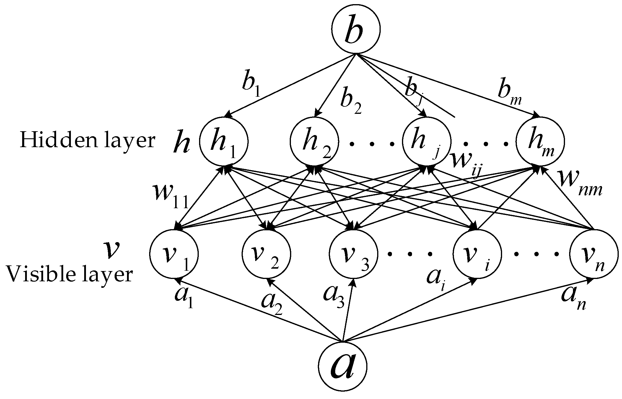
The DBN consists of stacked multilevel RBMs, which are based on the energy function definition and are the key preprocessing units in the field of deep learning. The RBM model is designed to fit the input data with maximum probability and train its hidden layer to capture high-order correlations in the input data. As shown in Figure 1, RBM consists of a hidden layer and a visible layer. A connection exists between each neuron node in the adjacent layers, and no connection exists within the same layer. Let $v=\{v_1,v_2,\cdots ,v_i,\cdots ,v_n\}$ denote the visible neuron nodes’ states in the visible layer, and $h=\{h_1,h_2,\cdots ,h_j,\cdots ,h_m\}$ show the hidden neurons’ states in the hidden layer.

Figure 1. Architecture of a Restricted Boltzmann Machine (RBM).

The neuron of an RBM is Boolean, i.e., there are only two states, 0 and 1. State 1 means that the neuron is activated, and state 0 means that the neuron is inhibited. The energy function [26] for a certain number of neuronal states is expressed as follows:

$$E(v,h;\theta )=-{\displaystyle \sum _{i=1}^n{\displaystyle \sum _{j=1}^m{w}_{ij}{v}_i{h}_j-{\displaystyle \sum _{i=1}^n{a}_i{v}_i-{\displaystyle \sum _{j=1}^m{b}_j{h}_j}}}}$$

(1)

where the RBM model parameters $\theta =\{W,a,b\}$, $a_i$ is the offset gradient of the visible layer, $b_j$ the offset gradient of the hidden layer. $v_i$ is the status of the $i^{th}$ neuron in the visual layer. $h_j$ is the status of the $j^{th}$ hidden neuron. $w_{ij}$ is the connection weight between the $i^{th}$ visible neuron and the $j^{th}$ hidden neuron.

According to the Equation (1), the joint probability distribution of visual neurons and hidden neurons is defined as follows:

$$P(v,h;\theta )=\frac{1}{Z(\theta )}\exp (-E(v,h;\theta ))$$

(2)

Let $Z(\theta )$ denote the normalization factor, which is expressed as:

$$Z(\theta )={\displaystyle \sum _v{\displaystyle \sum _h\exp (-E(v,h;\theta ))}}$$

(3)

Thus, the edge probability and conditional probability of visual and hidden neurons can be acquired, as follows:

$$\begin{array}{l}P(v;\theta )=\frac{{\displaystyle \sum _h\exp (-E(v,h;\theta ))}}{{\displaystyle \sum _v{\displaystyle \sum _h\exp (-E(v,h;\theta ))}}}\\ P(v|h;\theta )=\frac{\exp (-E(v,h;\theta ))}{{\displaystyle \sum _v\exp (-E(v,h;\theta ))}}\end{array}$$

(4)

$$\begin{array}{l}P(h;\theta )=\frac{{\displaystyle \sum _v\exp (-E(v,h;\theta ))}}{{\displaystyle \sum _v{\displaystyle \sum _h\exp (-E(v,h;\theta ))}}}\\ P(h|v;\theta )=\frac{\exp (-E(v,h;\theta ))}{{\displaystyle \sum _h\exp (-E(v,h;\theta ))}}\end{array}$$

(5)

The $j^{th}$ hidden neuron is activated with the probability calculated by:

$$\begin{array}{ll}p(h_j=1|v;\theta )& =\frac{{\displaystyle \sum _{h_{k¹j}}p(h_j=1,h_{k¹j},v;\theta )}}{{\displaystyle \sum _{h}p(h,v;\theta )}}\\ & =\sigma ({\displaystyle {\sum }_{i=1}^n{w}_{ij}{v}_i}+b_j)\end{array}$$

(6)

where $\sigma =1/(1+e^{-x})$ named sigmoid function is used here. Analogously, the $i^{th}$ visual neuron is activated with the probability calculated by:

$$\begin{array}{ll}p(v_i=1|h;\theta )& =\frac{{\displaystyle \sum _{v_{k¹i}}p(v_i=1,v_{k¹i},h;\theta )}}{{\displaystyle \sum _{v}p(v,h;\theta )}}\\ & =\sigma ({\displaystyle {\sum }_{j=1}^m{w}_{ij}{h}_j}+a_i)\end{array}$$

(7)

In the training RBM process, the visible neurons’ edge probability in the Gibbs distribution should be as close as possible to the input data distribution. Thus, the parameters $\theta$ are optimized to maximize the edge probability $P(v;\theta )$, the related logarithmic likelihood function is shown as:

$${\theta }^{*}=\underset{\theta }{\arg \max }L(\theta )=\underset{\theta }{\arg \max }{\displaystyle {\sum }_v\ln P(v;\theta )}$$

(8)

To acquire the optimal parameters ${\theta }^{*}$, the log-likelihood function of RBM is maximized by the stochastic gradient descent technique. The partial derivative of the log-likelihood function with respect to the parameter is:

$$\frac{\partial \ln p(v;\theta )}{\partial \theta }={⟨-\frac{\partial E(v,h;\theta )}{\partial \theta }⟩}_{p(h|v;\theta )}-{⟨-\frac{\partial E(v,h;\theta )}{\partial \theta }⟩}_{p(v,h;\theta )}$$

(9)

where ${⟨\cdot ⟩}_p$ represents mathematical expectations about distribution p, and $p(h|v;\theta )$ indicates the probability distribution of the hidden layer, while the training data are known. The parameters w, a, and b in $\theta$ are expressed as follows:

$$\frac{\partial \ln p(v;\theta )}{\partial w_{ij}}=p(h_j=1|v;\theta )v_i-{\displaystyle \sum _{v}p(v;\theta )}p(h_j=1|v;\theta )v_i$$

(10)

$$\frac{\partial \ln p(v;\theta )}{\partial a_i}=v_i-{\displaystyle \sum _{v}p(v;\theta )}{v}_i$$

(11)

$$\frac{\partial \ln p(v;\theta )}{\partial b_j}=p(h_j=1|v;\theta )-{\displaystyle \sum _{v}p(v;\theta )}p(h_j=1|v;\theta )$$

(12)

Owing to the symmetry of the RBM and the conditional independence of the neurons, a random sample of the distribution obeying the RBM definition can be obtained using the Gibbs sampling method. The $k$-step Gibbs sampling method aims to initialize the state $v^{(0)}$ of the visible neuron with a training sample (or a random state of the visible layer) and alternately perform the following sampling steps:

$$\{\begin{array}{c}{h}^{\left(i\right)}=G\left(p\left(h|v^{\left(i-1\right)}\right)\right)\\ v^{\left(i\right)}=G\left(p\left(v|h^{\left(i-1\right)}\right)\right)\end{array},i=1,2,\cdots ,k$$

(13)

where G(·) represents the operation of Gibbs sampling. $h^{\left(i\right)}$ and $v^{\left(i\right)}$ represent the intermediate results of h and v, respectively. When the number of sampling steps is large enough, a sample of the Gibbs distribution obeying the RBM representation can be obtained, and the gradient can be estimated by the following formula:

$$\begin{array}{ll}\frac{\partial \ln p(v;\theta )}{\partial w_{ij}}& =p(h_j=1|v;\theta )v_i-{\displaystyle \sum _{v}p(v;\theta )}p(h_j=1|v;\theta )v_i\\ & =p(h_j=1|v;\theta )v_i-p(h_j=1|v^{(k)};\theta )v_i^{(k)}\end{array}$$

(14)

$$\begin{array}{ll}\frac{\partial \ln p(v;\theta )}{\partial a_i}& =v_i-{\displaystyle \sum _{v}p(v;\theta )}{v}_i\\ & =v_i-v_i^{(k)}\end{array}$$

(15)

$$\begin{array}{ll}\frac{\partial \ln p(v;\theta )}{\partial b_j}& =p(h_j=1|v;\theta )-{\displaystyle \sum _{v}p(v;\theta )}p(h_j=1|v;\theta )\\ & =p(h_j=1|v;\theta )-p(h_j=1|v^{(k)};\theta )\end{array}$$

(16)

Typically, the large number of sampling steps leads to low training efficiency of RBM, especially when the characteristics of the training samples are large. Hinton [27] proposed the contrastive divergence fast training algorithm. In this algorithm, the state of the visual neuron is first set to the training sample, and then the binary state of all hidden layer neurons are calculated via Gibbs sampling. Equation (7) and Gibbs sampling are applied to determine the state of the visible layer neurons to obtain $v^{(1)}$. Generally, $v^{(1)}$ is sufficient to estimate the gradient. The update criterion for parameter $\theta =\{W,a,b\}$ is the following:

$$\begin{array}{l}{W}_{ij}^{\left\{t\right\}}\leftarrow W_{ij}^{\{t-1\}}+{\eta }_w({⟨v_i{h}_j⟩}_{data}^0-{⟨v_i{h}_j⟩}_{recon}^1)\\ a_i^{\left\{t\right\}}\leftarrow a_i^{\{t-1\}}+{\eta }_a({⟨v_i⟩}_{data}^0-{⟨v_i⟩}_{recon}^1)\\ b_j^{\left\{t\right\}}\leftarrow b_j^{\{t-1\}}+{\eta }_b({⟨h_j⟩}_{data}^0-{⟨h_j⟩}_{recon}^1)\end{array}$$

(17)

where ${\eta }_w$ is the learning rate of connection weight $w$, ${\eta }_a$ is the learning rate of visual layer deviation value $a$, and ${\eta }_b$ is the learning rate of hidden layer deviation value $b$, their values range from 0 to 1. ${⟨·⟩}_{data}$ stands for the original distribution of the data, ${⟨\cdot ⟩}_{recon}$ represents the distribution of model definitions after a one-step Gibbs sampling.

2.2. Deep Belief Networks

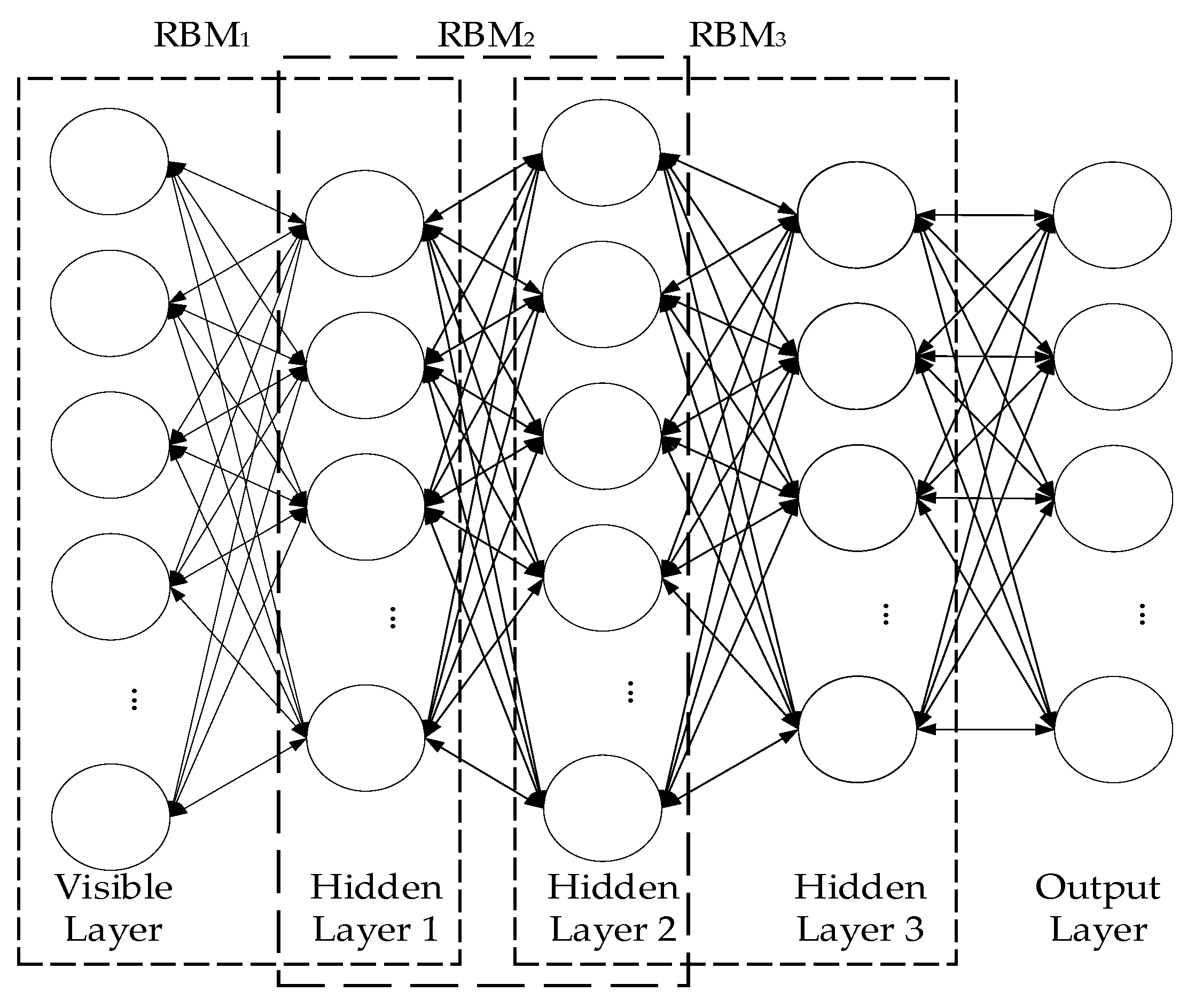
Actually, efficiently simulating complex raw data using only one RBM model is difficult. Therefore, constructing a DBN model stacked with a plurality of RBM models is necessary. Hinton et al. [28] put forward a fast learning algorithm for DBNs, which is essentially a stack of several RBM layers. DBN is a versatile deep learning model that can be used in unsupervised feature dimensionality reduction and supervised pattern classification. Whether supervised or unsupervised, DBN is essentially a series of feature learning processes to ensure improved feature representation. Similar to RBM, DBN is a probability stochastic model that aims to learn the joint probability distribution between the data from input and the hidden layer. Then, DBN correspondingly fits the data by adjusting the connection weight between every two adjacent layers of neuron nodes. The characteristic information is contained in the original input data.

In Figure 2, a stacked DBN model consists of three RBM layers is shown. The multi-hidden DBN model construction can be summed up as two parts: unsupervised pretraining phase and supervised form of global fine-tuning phase. The first part is pretraining, which is also called initialization parameters. One of the most difficult problems in traditional neural network training is how to select the appropriate initialization parameters. Although random initialization is commonly used, once the initialization parameters are randomly given, the final training and test results are seriously affected. To solve this problem, a pretraining technique based on a greedy layer-by-layer unsupervised learning algorithm is proposed. The DBN model is decomposed into a series of RBM models. The hidden layer state of each low-level RBM model is fed to its higher-level RBM model. The lowest state of the entire depth model is the original input data. Each parameter RBM model is trained successively to provide improved initialization weights and offset values for the entire DBN model.

Figure 2. Deep belief network (DBN) constructed by RBMs.

The second part is global fine-tuning. To further enhance the diagnostic capabilities of the model, after the unsupervised pretraining of a series of RBM models is complete, the original training data are used as the tag data to supervise the entire deep structure. According to the maximum likelihood function, the back propagation algorithm [29] is applied to further optimize the entire deep model and fine-tune the parameters of each layer. The DBN model has achieved very good application results on some public datasets, thereby proving that a suitable training technique is more conducive to obtaining improved initialization parameter values and global optimal solutions than traditional random initialization.

2.3. Momentum Method to Optimize Model Training

Stochastic gradient descent (SGD) and its variants may be the most widely used optimization algorithms in general machine learning, but the learning process is sometimes slow, and its update direction is completely dependent on the current batch. Thus, its update is highly unstable. A simple solution is to introduce a momentum.

The momentum method, which is also called classical momentum (CM), is a technique to accelerate gradient descent that accumulates velocity vectors in the direction where the objective lens continues to decrease during the iterative process. CM updates the direction of the preceding renewal and uses the gradient of the current batch to fine-tune the final update direction. Thus, stability can be increased to an extent, so that learning is fast. Based on the minimization of the objective function, the CM is given as follows:

$$\begin{array}{l}{v}_t=\gamma v_{t-1}+\eta {\nabla }_{\theta }J({\theta }_{t-1})\\ {\theta }_t={\theta }_{t-1}-v_t\end{array}$$

(18)

where $\theta$ represents DBN model parameters, $v_t$ represents the gradient after the end of t cycles, $v_{t-1}$ denotes the gradient after the end of the t-1 cycles, $\eta$ denotes the learning rate of RBM, $J(\theta )$ and ${\nabla }_{\theta }$ represent error function and the partial derivative of the error function compared with the model parameters, respectively. $\gamma \in [0,1]$ is the momentum coefficient that is usually set to 0.9 and, $\eta >0$ is the learning rate.

Using the SGD with the momentum causes the gradients in the same direction to accumulate, as those in various directions cancel each other, which can speed up the approach to the optimal point. Nonetheless, the gradient of the momentum technique is sightless. The gradient drops fast but cannot judge where the parameters will fall. As a result, the parameter still drops so fast when it is near the optimal solution that it may miss it. In this case, NM [30] can be a potential solution. The difference between NM and momentum is reflected in the gradient calculation. In NM, the gradient is calculated after the current speed is applied. Therefore, NM can be explained by adding a correction factor to the momentum method, which calculates the gradient of $J\left(\theta -\gamma v_{t-1}\right)$, to calculate the location of the parameter’s next drop. This situation slows down the drop before the parameters reach their optimal point, so that missing this point can be avoided.

$$\begin{array}{l}{v}_t=\gamma v_{t-1}+\eta {\nabla }_{\theta }J({\theta }_{t-1}-\gamma v_{t-1})\\ {\theta }_t={\theta }_{t-1}-v_t\end{array}$$

(19)

2.4. Individual Adaptive Learning Rate to Accelerate Model Convergence

However, the NM method is sometimes extremely conservative [31]. An independent adaptive learning rate is introduced to the RBM training to achieve the satisfactory classification and training speed. $w_{ij}$ is updated by:

$$h_{ij}(k)=\{\begin{array}{l}{h}_{ij}(k-1)+\alpha \hspace{1em}\hspace{1em}\hspace{1em}if(gra{d}_{ij}^{k}gra{d}_{ij}^{k-1})>0\\ h_{ij}(k-1)\times (1-\alpha ) if(gra{d}_{ij}^{k}gra{d}_{ij}^{k-1})<0\end{array}$$

(20)

$$\Delta w_{ij}^k=\eta \cdot h_{ij}^k\cdot {\nabla }_{\theta }J({\theta }_{t-1}-\gamma v_{t-1})$$

(21)

where $gra{d}_{ij}^k$ indicates the gradient of $w_{ij}$ after the kth training, $h_{ij}(0)=1$. When the gradient direction of the present weight keeps the same as the previous one, $h_{ij}(t)$ increases $\alpha$ times. Inversely, $h_{ij}(t)$ is decreased $1-\alpha$ times. The parameter $\alpha$ can be set as 0.1, so that it is small enough to guarantee that the learning rate will not increase too fast, which may cause the miss of the optimal point. The range of $h_{ij}(t)$ should be limited to [0.01, 100] to prevent gradient disappearance.

The proposed training method can avert the problem of negative acceleration of the training speed of the model during the training process. It compensates the gradient update to a certain extent by enhancing the falling step size to guarantee that the parameters get higher training speed without missing the optimal solution when the NM method judges falsely.

3. Improved Hierarchical Adaptive Deep Belief Network for Bearing Fault Diagnosis

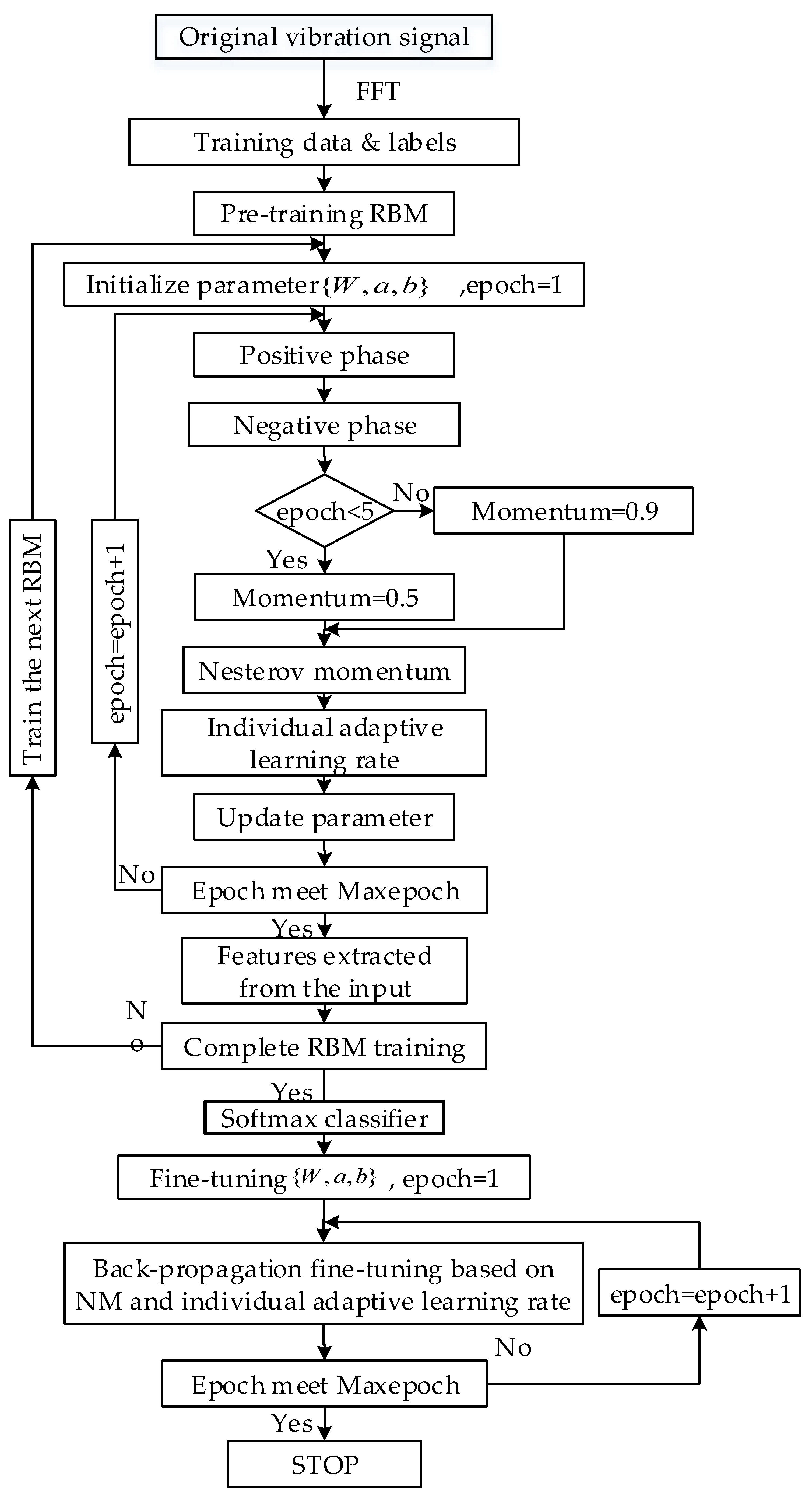
On the basis of the classical DBN model and its improvements, a hierarchical adaptive DBN is established. Figure 4 shows the flowchart of the DBN training. The DBN initialization is done by training each RBM through a greedy layer-by-layer unsupervised algorithm and untagged training sample sets. The initialized Softmax classifier is connected to the top of the model as the classification layer. The NM and independent adaptive learning rate are employed to assist the DBN model construction.

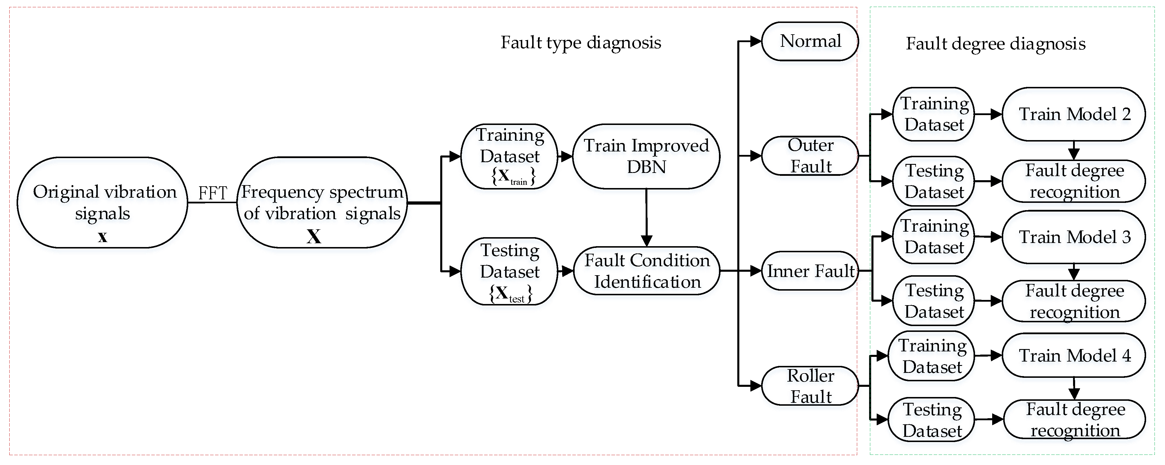
Figure 3 shows the hierarchical fault diagnosis model. The training and testing samples are obtained in the frequency domain by Fast Fourier Transform (FFT). The whole training samples are utilized in the training of the improved DBN model (model 1) to classify the bearing fault type, and a fault-type diagnostic layer is formed. Then, the improved DBN sub-models (models 2, 3, and 4) are created for each fault type, so that the respective models can recognize the fault degree. Similarly, a fault degree recognition layer is constructed. For each model, the testing samples are prepared for performance validation. Figure 4 illustrates the training process of the raised model.

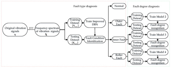
Figure 3. Flowchart of hierarchical fault diagnosis method.

Figure 4. Training process of proposed DBN model.

4. Experimental Analysis

4.1. Test Rig and Dataset Introduction

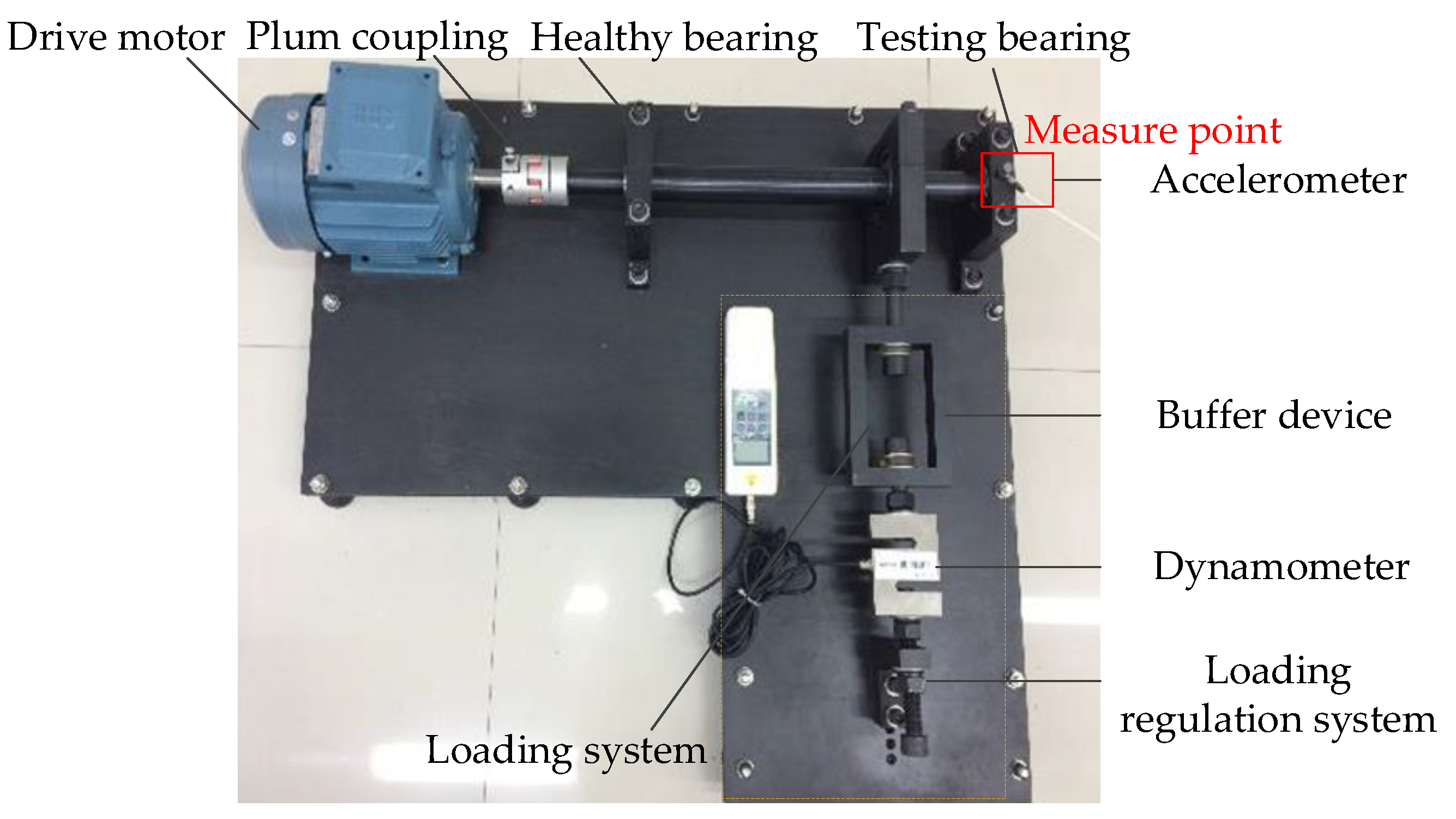
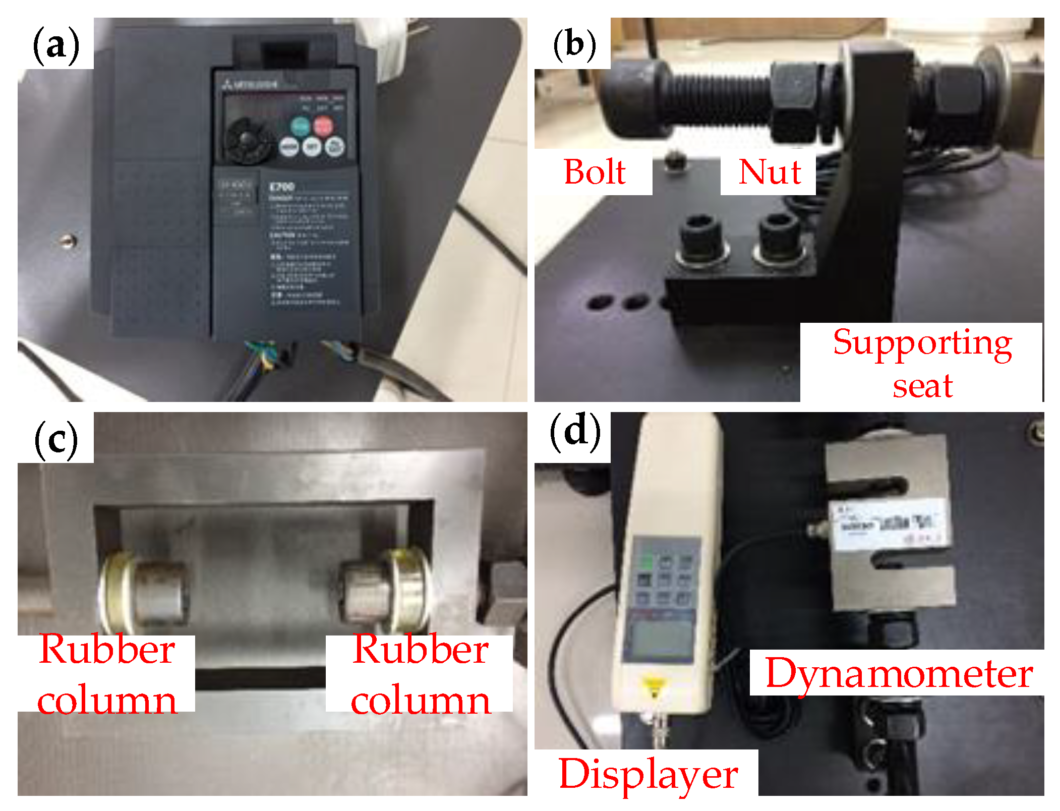
Figure 5 shows the experimental platform including motor, inverter, normal and testing bearings, loading regulation system, vibration acceleration sensor, and data acquisition system. The inverter motor is the power input of the platform. The 6205-2RS SKF bearing was tested and its parameters are listed in Table 1. The accelerometer was placed as indicated by the red box in Figure 5. The nut was squeezed against the support seat, and a radial load could be adjusted by the nut, as Figure 6b–d shows. The load was transmitted to the testing bearing through the visible dynamometer, buffer device, and drive shaft. The running speed of the motor was set as 961 rpm. The load was set as 0.2 kN, and the signal sampling frequency was 10 kHz. In order to ensure that each sample contained enough fault information, each sample was selected to cover 1248 data points.

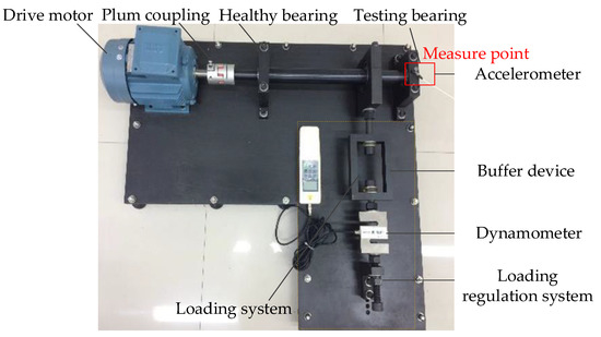
Figure 5. Bearing test rig.

Table 1. Specifications of testing bearing.

Contact Angle (°)	Roller Diameter (mm)	Roller Number	Pitch Diameter (mm)	Inner Diameter (mm)	Outer Diameter (mm)
0	7.938	9	38.5	25	52

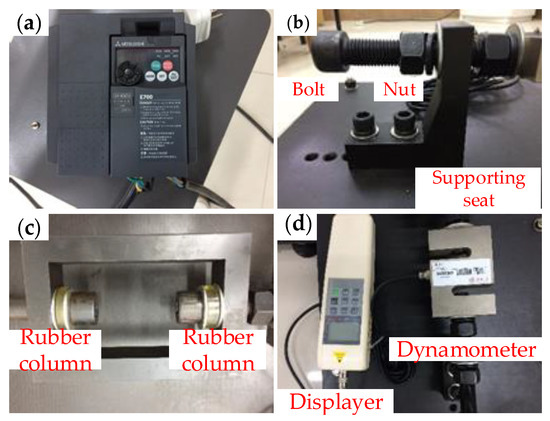
Figure 6. Platform components: (a) inverter and (b–d) loading regulation system.

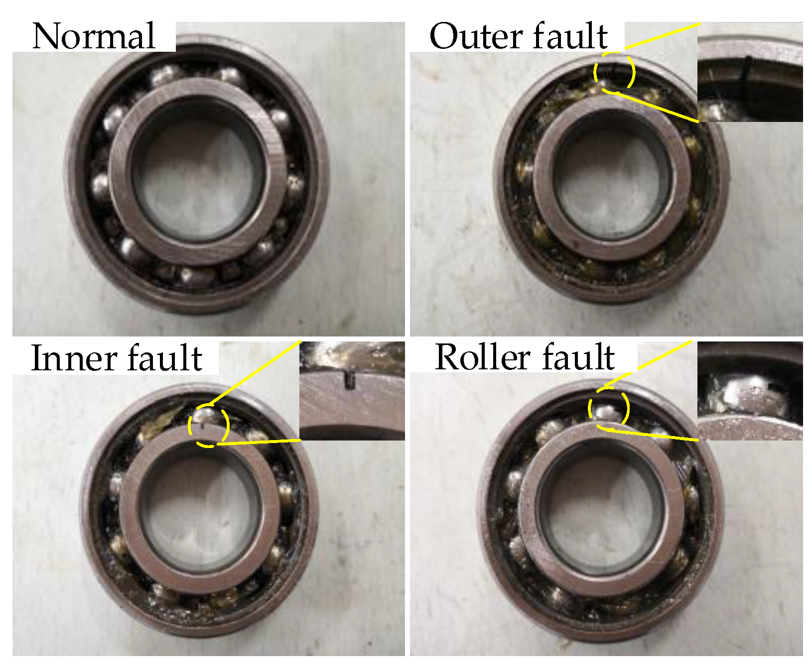
Spark-erosion wire cutting was conducted before the experiment, to set up multiple types of single-point faults on the testing bearing surface. The physical object is shown in Figure 7. Experiments under 13 health conditions were carried out, as listed in Table 2, including four fault types and four fault degrees.

Figure 7. Physical pictures of fault bearing.

Table 2. Description of dataset for hierarchical fault diagnosis model.

Identification Label		Number of Training Samples	Number of Testing Samples
Fault Type	Fault Degree
Normal: 1	\	64	16
Outer fault: 2	0.2 mm: 1 0.3 mm: 2 0.4 mm: 3 0.5 mm: 4	75	25
Inner fault: 3	0.2 mm: 1 0.3 mm: 2 0.4 mm: 3 0.5 mm: 4	75	25
Roller fault: 4	0.2 mm: 1 0.3 mm: 2 0.4 mm: 3 0.5 mm: 4	75	25

For analysis, part of the whole samples were selected for testing, and the other samples were used for training. Corresponding labels for various fault-state sample sets were defined to construct the recognition models. Table 2 summarizes the dataset details.

For the hierarchical fault diagnosis, each model included a visible layer and two hidden layers. Among them, there were 624 neurons in the visible layer and 500 neurons in the first hidden layer. The number of hidden layer neurons in the second layer was 200, in which the numbers of diagnostic layers of fault types and the degrees were 4. The connection weights $W$ of each layer, $W~N(0,0.01)$ were initialized. The learning rates in these two RBMs were initialized to 0.1 and 0.0025. To reduce the impact of random factors and achieve enhanced results, various iterations were conducted on the four improved DBN models, and the selected parameters are listed in Table 3.

Table 3. Selection of parameters for hierarchical fault diagnosis model.

Network Model	Network Structure	Initial Learning Rate
		1st RBM	2nd RBM
Model 1	624-500-200-4	0.1	0.0025
Model 2	624-500-200-5	0.1	0.0025
Model 3	624-500-200-5	0.1	0.0025
Model 4	624-500-200-5	0.1	0.0025

4.2. Experimental Validation

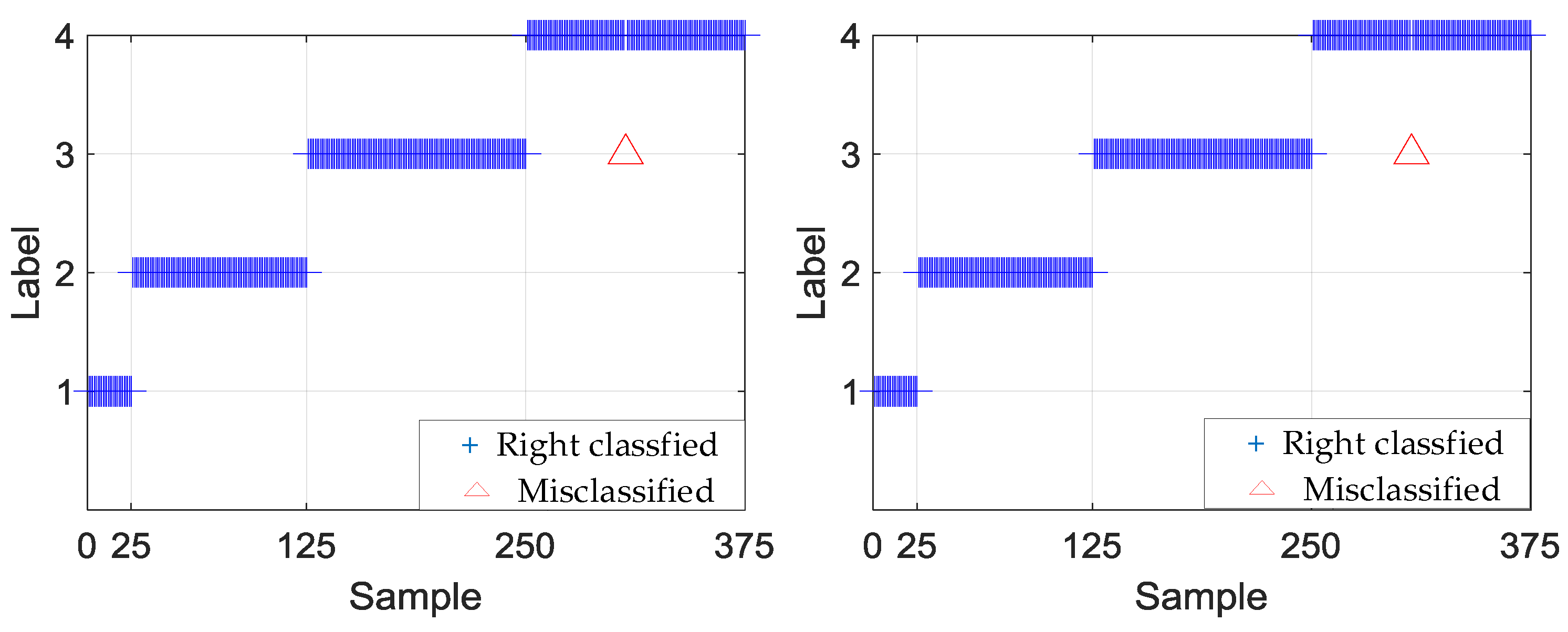
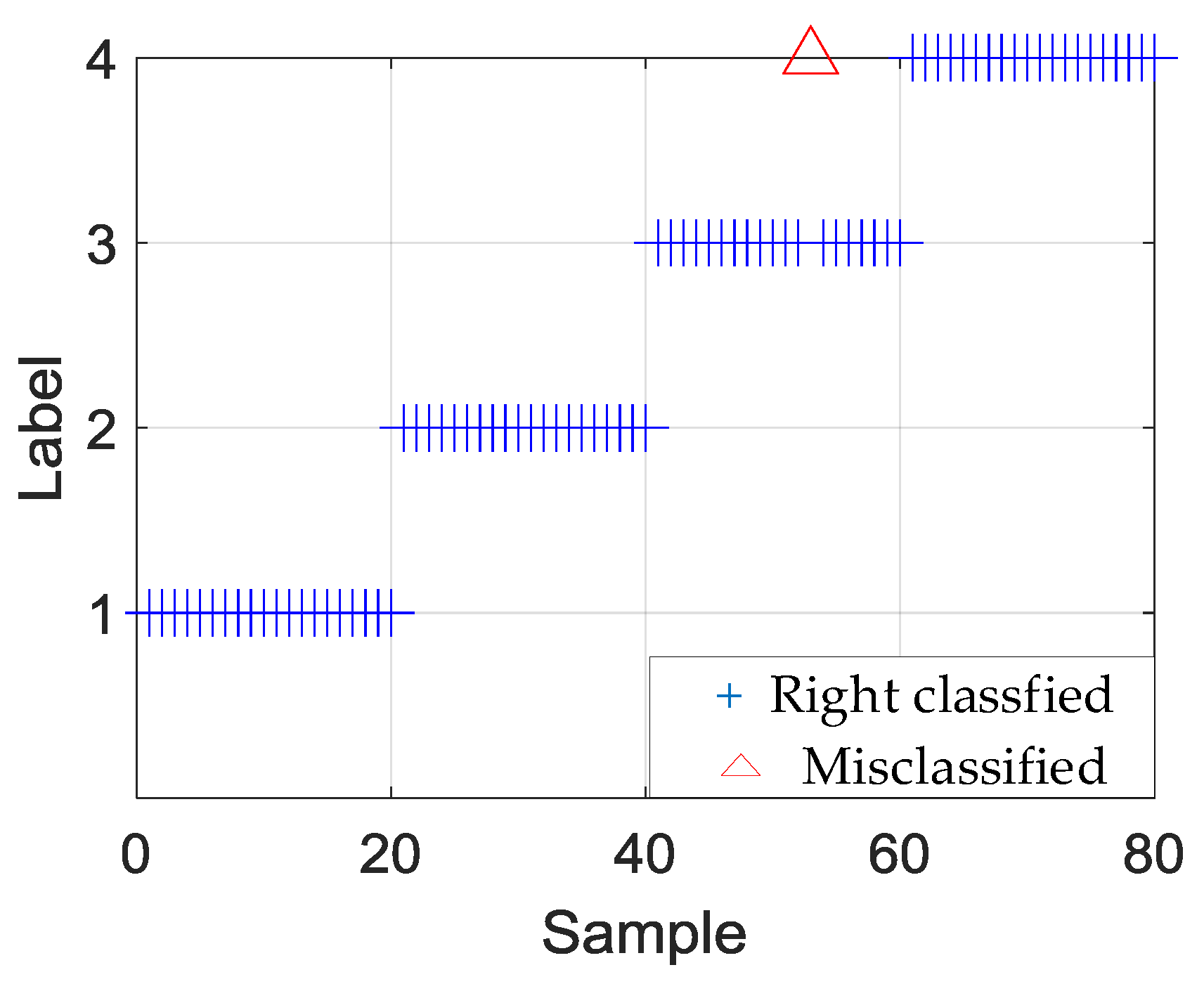
Table 4, Table 5, Table 6 and Table 7 show the testing results of the hierarchical fault diagnosis model. Table 4 presents the fault-type identified results. According to Table 4, model 1 can accurately identify the bearing fault type. The average test accuracy of the 10 experiments was 99.95%. Figure 8 shows the specific fault-type identification results of experiments 2 and 6. In experiment 2, a roller fault sample was misclassified as an inner fault. Experiment 6 exhibited the same result. Table 5, Table 6 and Table 7 show the fault-degree identification results in outer race, roller, and inner race, respectively.

Table 4. Testing results of model 1 in hierarchical fault diagnosis.

Experiment Number	Fault Type
	Inner Fault	Outer Fault	Roller Fault	Normal	Average
1	100%	100%	100%	100%	100%
2	100%	100%	99%	100%	99.75%
3	100%	100%	100%	100%	100%
4	100%	100%	100%	100%	100%
5	100%	100%	100%	100%	100%
6	100%	100%	99%	100%	99.75%
7	100%	100%	100%	100%	100%
8	100%	100%	100%	100%	100%
9	100%	100%	100%	100%	100%
10	100%	100%	100%	100%	100%

Table 5. Testing results of outer fault degree recognition by hierarchical fault diagnosis model.

Experiment Number	Fault Degree Recognition (mm)
	0.2	0.3	0.4	0.5	Average
1	100%	100%	100%	100%	100%
2	100%	100%	100%	100%	100%
3	100%	100%	100%	100%	100%
4	100%	100%	100%	100%	100%
5	100%	100%	100%	100%	100%
6	100%	100%	100%	100%	100%
7	100%	100%	100%	100%	100%
8	100%	100%	100%	100%	100%
9	100%	100%	100%	100%	100%
10	100%	100%	100%	100%	100%

Table 6. Testing results of roller fault degree recognition by hierarchical fault diagnosis model.

Experiment Number	Fault Degree Recognition (mm)
	0.2	0.3	0.4	0.5	Average
1	100%	100%	96%	100%	99%
2	100%	100%	100%	100%	100%
3	100%	100%	100%	100%	100%
4	100%	100%	100%	100%	100%
5	100%	100%	100%	100%	100%
6	100%	100%	100%	100%	100%
7	100%	100%	100%	100%	100%
8	100%	100%	100%	100%	100%
9	100%	100%	100%	100%	100%
10	100%	100%	100%	100%	100%

Table 7. Testing results of inner fault degree recognition by hierarchical fault diagnosis model.

Experiment Number	Fault Degree Recognition (mm)
	0.2	0.3	0.4	0.5	Average
1	100%	100%	100%	100%	100%
2	100%	100%	100%	100%	100%
3	100%	100%	100%	100%	100%
4	100%	100%	100%	100%	100%
5	100%	100%	100%	100%	100%
6	100%	100%	100%	100%	100%
7	100%	100%	100%	100%	100%
8	100%	100%	100%	100%	100%
9	100%	100%	100%	100%	100%
10	100%	100%	100%	100%	100%

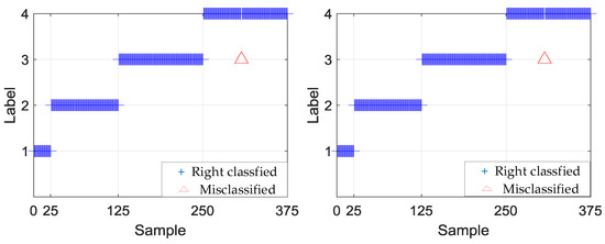
Figure 8. Identification results of experiments 2 and 6.

For the bearing faults, models 2, 3, and 4 can identify the fault degree satisfactorily. The accuracy of the 10 experimental tests of outer and roller fault degrees reached 100%. In the 10 experiments for the inner fault size identification, the testing accuracy of the first experiment was 99%, and that of the other 9 experiments was 100%. Figure 9 shows the results of the inner fault size identification of experiment 1, in which an inner fault of size 0.4 mm was classified as 0.5 mm.

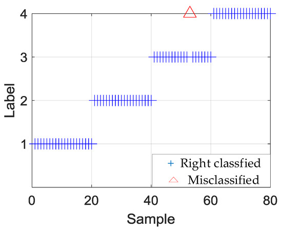
Figure 9. Experiment 1 of inner fault degree recognition.

Table 8 and Table 9 list the comparisons among three methods. It can be seen that the proposed approach achieved better performance. The generalizability of the DBN model has been improved, to guarantee the convergence speed effectively and achieve an optimal point, thereby achieving increased precision. As illustrated in Table 9, the raised approach also obtained outstanding results.

Table 8. Training accuracy results of various methods.

Methods	Normal	Outer Fault	Roller Fault	Inner Fault	Average Training Accuracy
Support Vector Machine (SVM)+FFT	100%	100%	98.688%	100%	99.672%
Standard DBN+FFT	90.159%	100%	99.034%	100%	97.298%
The proposed method	100%	100%	99.167%	100%	99.790%

Table 9. Testing accuracy results of various methods.

Methods	Normal	Outer Fault	Roller Fault	Inner Fault	Average Testing Accuracy
SVM+FFT	91.154%	100%	91.250%	98.750%	95.290%
Standard DBN+FFT	98.900%	100%	99.500%	99.600%	99.500%
The proposed method	99.950%	100%	100%	99.900%	99.960%

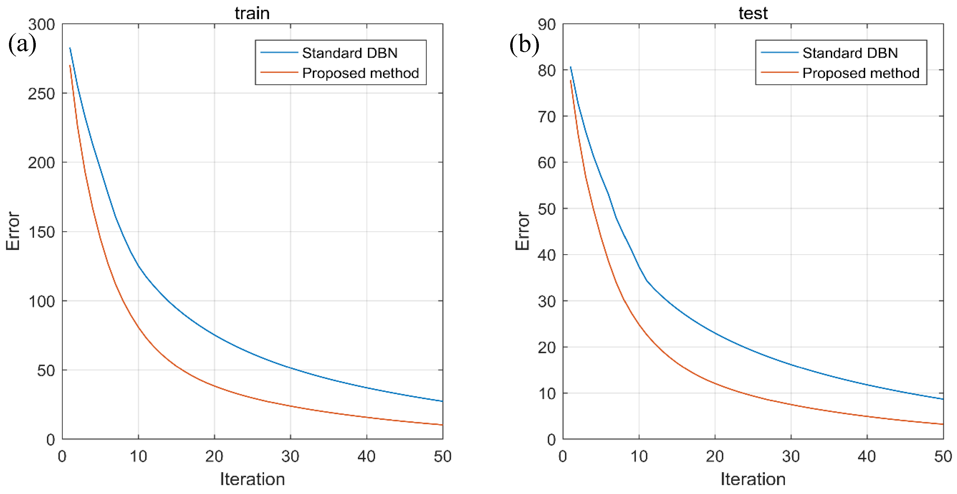
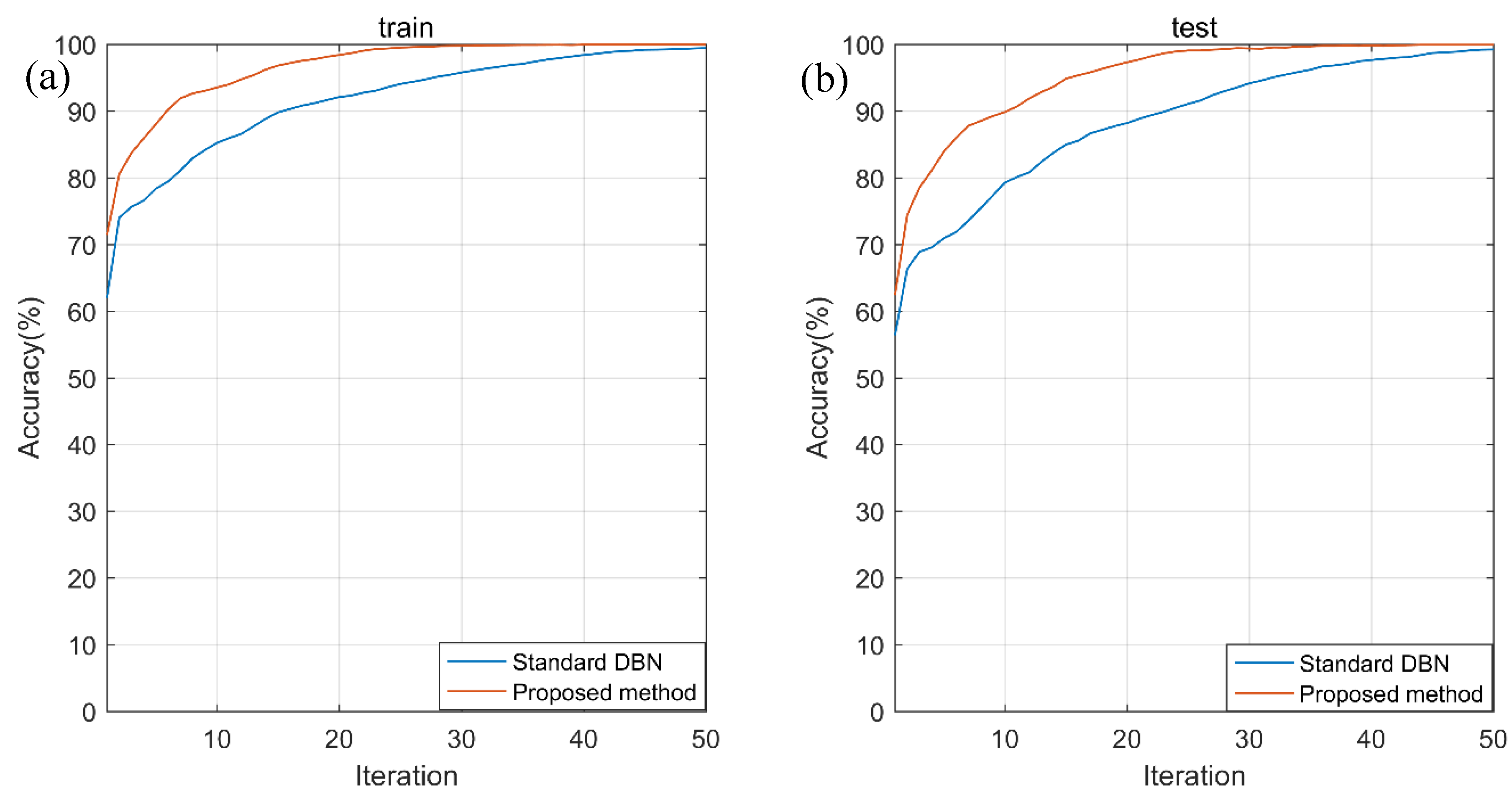
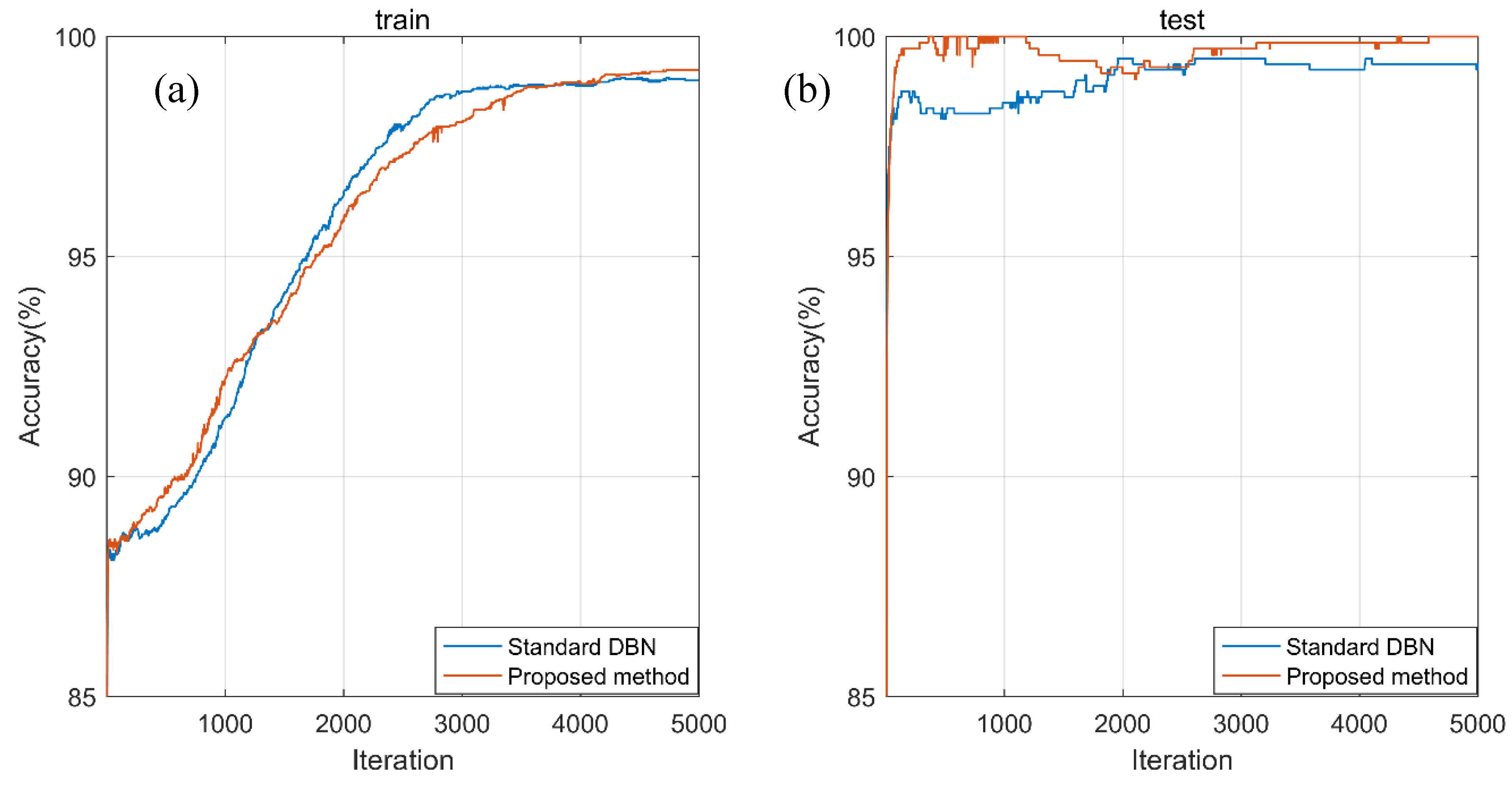
Taking the fault type identification as an example, Figure 10 depicts the errors’ trends of training and testing models in the global fine-tuning iterations and shows satisfactory convergence trends. Figure 11 shows the training and testing accuracy trends of fault type recognition in the global fine-tuning iterations. It can be clearly seen that the proposed method can achieve faster convergence and higher accuracy, compared with standard DBN. Similarly, Figure 12 generally exhibits desirable accuracy improvements of the proposed method for roller fault degree recognition.

Figure 10. Errors’ trends of (a) training and (b) testing models for identifying fault type.

Figure 11. Accuracies’ trends of (a) training and (b) testing models for identifying fault type.

Figure 12. Accuracy trends of (a) training and (b) testing models for roller fault degree recognition.

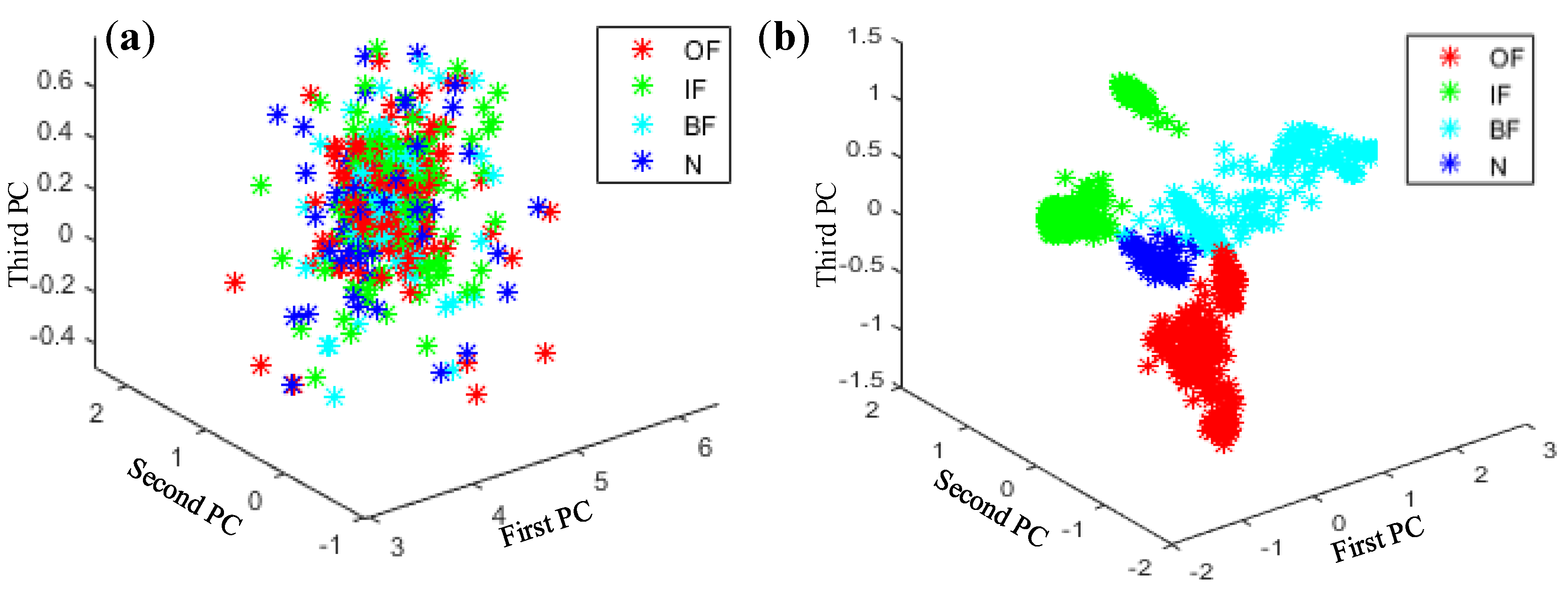
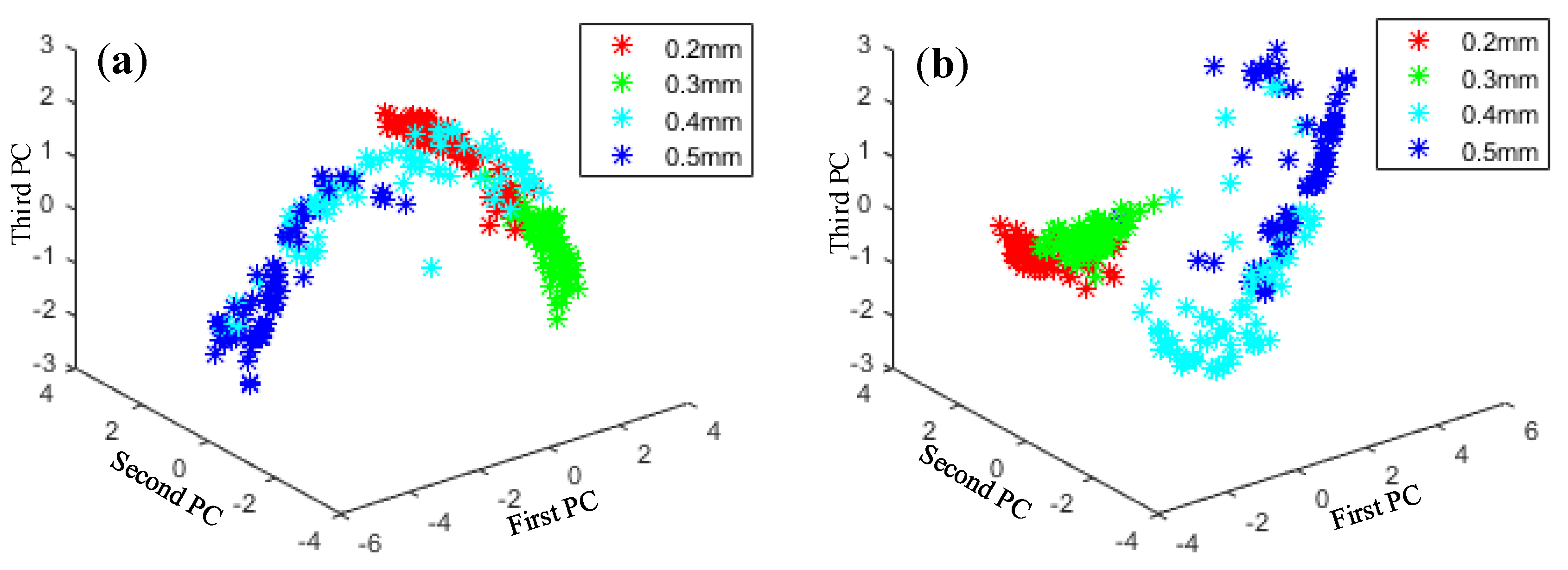
Principal component analysis (PCA) is a typical method for dimensionality reduction and has been widely used in fields such as data noise cancellation and data compression to eliminate redundancy. As shown in Figure 13, Figure 14, Figure 15 and Figure 16, PCA was used to visualize features obtained by the proposed method. The clustering performance of the original signal was not good, and the characteristics of each fault type were mixed and difficult to distinguish. The reason for these improvements may be that the proposed adaptive DBN based on the NM method has stronger classification ability than the traditional SVM shallow layer network, thereby effectively realizing bearing fault diagnosis. The independent adaptive learning rate can effectively optimize the generalizability of the DBN and ensure the representativeness of the deep features of the extracted data. Generally, the hierarchical fault diagnosis network gets desirable outcomes and performs better than traditional methods.

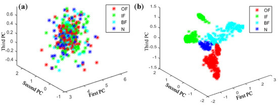
Figure 13. Feature visualization of signals under various fault types: (a) raw data features and (b) proposed method.

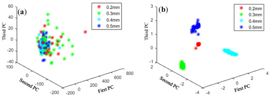
Figure 14. Feature visualization of various outer fault degrees: (a) raw data features and (b) proposed method.

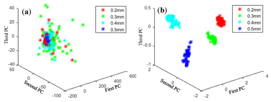
Figure 15. Feature visualization of various inner fault degrees: (a) raw data features and (b) proposed method.

Figure 16. Feature visualization of various roller fault degrees: (a) raw data features and (b) proposed method.

5. Conclusions

Motivated by the fact that conventional fault diagnosis methods rely on the representational capacity of the manually extracted features, and the parameters selection may affect the performance of models, this research presents a new hierarchical bearing fault diagnosis method. The NM is adapted to the DBN training process to directly extract deep data features from frequency domain signals. Besides, a learning rate adjustment strategy is introduced to complete the optimization process of parameter updating. These improvements can effectively enhance the generalizability of the DBN, ensure representativeness of the learned features, and finally, achieve the bearing fault type identification as well as its degree. Through experimental verification, the improved hierarchical adaptive DBN can learn from data to obtain deep features automatically and achieve satisfactory accuracies of fault diagnosis at a more efficient speed than those obtained by traditional methods.

References

- Wang, H.; Wang, P.; Song, L.; Ren, B.; Cui, L. A Novel Feature Enhancement Method Based on Improved Constraint Model of Online Dictionary Learning. IEEE Access 2019, 7, 17599–17607. [Google Scholar] [CrossRef]
- Islam, M.R.; Uddin, M.S.; Khan, S.; Kim, J.M.; Kim, C.H. Multi-core Accelerated Discriminant Feature Selection for Real-Time Bearing Fault Diagnosis. In Trends in Applied Knowledge-Based Systems and Data Science, Proceedings of the International Conference on Industrial, Engineering and Other Applications of Applied Intelligent Systems, Morioka, Japan, 2–4 August 2016; Springer: Cham, Switzerland, 2016; Volume 9799, pp. 645–656. [Google Scholar]
- Li, C.; Tao, Y.; Ao, W.; Yang, S.; Bai, Y. Improving forecasting accuracy of daily enterprise electricity consumption using a random forest based on ensemble empirical mode decomposition. Energy 2018, 165, 1220–1227. [Google Scholar] [CrossRef]
- Li, Z.; Ming, A.; Zhang, W.; Liu, T.; Chu, F.; Li, Y. Fault Feature Extraction and Enhancement of Rolling Element Bearings Based on Maximum Correlated Kurtosis Deconvolution and Improved Empirical Wavelet Transform. Appl. Sci. 2019, 9, 1876. [Google Scholar] [CrossRef]
- He, Q.; Wu, E.; Pan, Y. Multi-scale stochastic resonance spectrogram for fault diagnosis of rolling element bearings. J. Sound Vib. 2018, 420, 174–184. [Google Scholar] [CrossRef]
- Wang, Y.; Markert, R.; Xiang, J.; Zheng, W. Research on variational mode decomposition and its application in detecting rub-impact fault of the rotor system. Mech. Syst. Sig. Process. 2015, 60, 243–251. [Google Scholar] [CrossRef]
- Wang, J.; Gao, R.X.; Yan, R. Integration of EEMD and ICA for wind turbine gearbox diagnosis. Wind Energy 2014, 17, 757–773. [Google Scholar] [CrossRef]
- Wang, D.; Tsui, K.L. Theoretical investigation of the upper and lower bounds of a generalized dimensionless bearing health indicator. Mech. Syst. Sig. Process. 2018, 98, 890–901. [Google Scholar] [CrossRef]
- Li, L.; Liang, X.; Xu, M.; Huang, W. Early fault feature extraction of rolling bearing based on ICD and tunable Q-factor wavelet transform. Mech. Syst. Sig. Process. 2017, 86, 204–223. [Google Scholar] [CrossRef]
- Gao, Y.; Villecco, F.; Li, M.; Song, W. Multi-Scale Permutation Entropy Based on Improved LMD and HMM for Rolling Bearing Diagnosis. Entropy 2017, 19, 176. [Google Scholar] [CrossRef]
- Arnaiz-González, Á.; Fernández-Valdivielso, A.; Bustillo, A.; de Lacalle, L.N.L. Using artificial neural networks for the prediction of dimensional error on inclined surfaces manufactured by ball-end milling. Int. J. Adv. Manuf. Technol. 2016, 83, 847–859. [Google Scholar] [CrossRef]
- Bustillo, A.; Urbikain, G.; Perez, J.M.; Pereira, O.M.; de Lacalle, L.N.L. Smart optimization of a friction-drilling process based on boosting ensembles. J. Manuf. Syst. 2018, 48, 108–121. [Google Scholar] [CrossRef]
- Islam, M.M.; Kim, J.M. Reliable multiple combined fault diagnosis of bearings using heterogeneous feature models and multiclass support vector Machines. Reliab. Eng. Syst. Saf. 2019, 184, 55–66. [Google Scholar] [CrossRef]
- Zhao, R.; Yan, R.; Chen, Z.; Mao, K.; Wang, P.; Gao, R.X. Deep learning and its applications to machine health monitoring. Mech. Syst. Sig. Process. 2019, 115, 213–237. [Google Scholar] [CrossRef]
- Shao, H.; Jiang, H.; Zhang, X.; Niu, M. Rolling bearing fault diagnosis using an optimization deep belief network. Meas. Sci. Technol. 2015, 26, 115002. [Google Scholar] [CrossRef]
- Guo, X.; Chen, L.; Shen, C. Hierarchical adaptive deep convolution neural network and its application to bearing fault diagnosis. Measurement 2016, 93, 490–502. [Google Scholar] [CrossRef]
- Qin, Y.; Wang, X.; Zou, J. The optimized deep belief networks with improved logistic Sigmoid units and their application in fault diagnosis for planetary gearboxes of wind turbines. IEEE Trans. Ind. Electron. 2019, 66, 3814–3824. [Google Scholar] [CrossRef]
- Zhang, W.; Peng, G.; Li, C. Bearings fault diagnosis based on convolutional neural networks with 2-D representation of vibration signals as input. In Proceedings of the 2016 the 3rd International Conference on Mechatronics and Mechanical Engineering, Shanghai, China, 21–23 October 2016; Yuan, H.L., Agarwal, R.K., Tandon, P., Wang, E.X., Eds.; EDP Sciences: Les Ulis, France, 2017; Volume 95, p. 5. [Google Scholar]
- Gan, M.; Wang, C.; Zhu, C. Construction of hierarchical diagnosis network based on deep learning and its application in the fault pattern recognition of rolling element bearings. Mech. Syst. Sig. Process. 2016, 72–73, 92–104. [Google Scholar] [CrossRef]
- Lu, C.; Wang, Z.Y.; Qin, W.L.; Ma, J. Fault diagnosis of rotary machinery components using a stacked denoising autoencoder-based health state identification. Signal Process. 2017, 130, 377–388. [Google Scholar] [CrossRef]
- Chen, Z.; Li, W. Multisensor feature fusion for bearing fault diagnosis using sparse autoencoder and deep belief network. IEEE Trans. Instrum. Meas. 2017, 66, 1693–1702. [Google Scholar] [CrossRef]
- Tang, S.; You, W.; Shen, C.; Shi, J.; Li, S.; Zhu, Z. A self-adaptive deep belief network with Nesterov momentum for the fault diagnosis of rolling element bearings. In Proceedings of the 2017 International Conference on Deep Learning Technologies, Chengdu, China, 2–4 June 2017; ACM: New York, NY, USA, 2017; pp. 1–5. [Google Scholar]
- Hamadache, M.; Jung, J.H.; Park, J.; Youn, B.D. A comprehensive review of artificial intelligence-based approaches for rolling element bearing PHM: Shallow and deep learning. JMST Adv. 2019, 1, 1–27. [Google Scholar] [CrossRef]
- Tao, J.; Liu, Y.; Yang, D. Bearing fault diagnosis based on deep belief network and multisensor information fusion. Shock Vibr. 2016, 2016, 1–9. [Google Scholar] [CrossRef]
- Shen, C.; Qi, Y.; Wang, J.; Cai, G.; Zhu, Z. An automatic and robust features learning method for rotating machinery fault diagnosis based on contractive autoencoder. Eng. Appl. Artif. Intell. 2018, 76, 170–184. [Google Scholar] [CrossRef]
- Qian, N. On the momentum term in gradient descent learning algorithms. Neural Netw. 1999, 12, 145–151. [Google Scholar] [CrossRef]
- Hinton, G.E. Training products of experts by minimizing contrastive divergence. Neural Comput. 2002, 14. [Google Scholar] [CrossRef]
- Hinton, G.E.; Osindero, S.; Teh, Y.W. A fast learning algorithm for deep belief nets. Neural Comput. 2006, 18, 1527–1554. [Google Scholar] [CrossRef] [PubMed]
- Zhao, Z.; Xu, Q.; Jia, M. Improved shuffled frog leaping algorithm-based BP neural network and its application in bearing early fault diagnosis. Neural Comput. Appl. 2016, 27, 375–385. [Google Scholar] [CrossRef]
- Kingma, D.P.; Ba, J. Adam: A method for stochastic optimization. arXiv 2014, arXiv:1412.6980. [Google Scholar]
- Tieleman, T.; Hinton, G. Lecture 6.5-rmsprop: Divide the gradient by a running average of its recent magnitude. COURSERA Neural Netw. Mach. Learn 2012, 4, 26–30. [Google Scholar]
© 2019 by the authors. Licensee MDPI, Basel, Switzerland. This article is an open access article distributed under the terms and conditions of the Creative Commons Attribution (CC BY) license (http://creativecommons.org/licenses/by/4.0/).