Abstract
Anomaly detection in crowded scenes is an important and challenging part of the intelligent video surveillance system. As the deep neural networks make success in feature representation, the features extracted by a deep neural network represent the appearance and motion patterns in different scenes more specifically, comparing with the hand-crafted features typically used in the traditional anomaly detection approaches. In this paper, we propose a new baseline framework of anomaly detection for complex surveillance scenes based on a variational auto-encoder with convolution kernels to learn feature representations. Firstly, the raw frames series are provided as input to our variational auto-encoder without any preprocessing to learn the appearance and motion features of the receptive fields. Then, multiple Gaussian models are used to predict the anomaly scores of the corresponding receptive fields. Our proposed two-stage anomaly detection system is evaluated on the video surveillance dataset for a large scene, UCSD pedestrian datasets, and yields competitive performance compared with state-of-the-art methods.
1. Introduction
With the wide use of video surveillance systems, the conventional manual analysis for labelling abnormal events in the amount of video data captured from crowd surveillance and public place monitoring is time-consuming and inefficient. Therefore, an intelligent surveillance system that can recognize and detect anomalies is urgently needed and has been a hotspot of computer vision researches and applications [1,2,3,4].
However, anomaly detection and localization is still a challenging problem in intelligent video surveillance, though some great progress has been made in feature extraction, behavior modeling, and anomaly measuring. The most challenging issue is that the definition of the anomaly is indefinite in most of the real-world surveillance videos. In general, events that are significantly different from common events are defined as anomalies, which means anomalies are defined by normal events instead of classifications or details of themselves. An event anomalous in one scene (such as a person running) may not be anomalous in a second scene, since the normal events in the second scene may include running people whereas the first does not. Therefore, anomalies are of insufficient sizes and similarities to be effectively modeled. Anomaly detection for crowd scene is essentially a novelty detection, which is also known as a one-class, semi-supervised learning problem [5,6,7], since the training data of the existing datasets contains only normal events while the data to be verified contains both normal and abnormal events.
Traditional solutions in the literature concentrated on the analysis of local or individual spatiotemporal patterns in the scene [8,9,10]. Therefore, various feature descriptors were designed to extract low-level features from the appearance and motion cues. Some works [11,12] used the popular low-level features including the histogram of oriented gradients (HOG), the 3D spatiotemporal gradients, and the histogram of oriented flows (HOF) to describe the patterns of the minimal units. However, adopting the hand-crafted generic feature extractors rather than specific descriptors learned from the scene is a clear limitation. Some other systems [5,13] were based on the analysis of the motion information in the scene. In these works, the local trajectories or the optical flows of the pixels were computed and modeled in order to describe the motion patterns. However, these approaches lacked stability when dealing with complex scenes, as the accuracy of the pixels trajectories extraction significantly degraded when a dynamic occlusion occurred among multiple objects.
Recently, deep learning approaches have achieved remarkable success in various computer vision tasks, such as object classification and object detection [14,15], and these applications were based on supervised learning that required labels. In the meantime, unsupervised learning based approaches such as auto-encoder and variational auto-encoder (VAE) have been widely used for feature extraction [16,17,18]. These works have shown that comparing with traditional methods, rich and specific features can be learned. Therefore, in the anomaly detection tasks, the hand-crafted feature extractors are now being replaced by the auto-encoders. Based on these learned features, some works reconstructed or generated a whole new frame by using a fully convolutional network (FCN) [19] and the total deviation between the generation and the original frame was used to predict the anomaly [6,20]. However, these methods can hardly locate abnormal events in frames. Some other works used probability estimation models, such as one-class SVM models [21] and Gaussian models [22], to predict the anomaly scores of the learned features. In these works, all the features shared the same model, even though they were extraced from different regions.
In this paper, we propose a baseline framework of an anomaly detection system for complex surveillance scenes by using a VAE with convolution kernels, which is inspired by the convolutional auto-encoder and the FCN architecture. In the first stage, the still frame series are provided as input to our VAE, then the appearance and motion features of the receptive fields, which are densely distributed throughout the frames, are extracted by the encoder network. In the second stage, comparing to the solutions based on reconstruction or generation, our system locates the anomalies by using multiple multivariate Gaussian models to predict the anomaly scores of each receptive field. Besides that, each multivariate Gaussian model is fitted to the corresponding feature representations, which means that the receptive fields at different loactions have their own Gaussian models. Futhermore, according to the principle of VAE, our feature vectors are more independent and decoupled than those extracted by original auto-encoders and convolutional auto-encoders. Then, an averaging operation is used to handle the overlapping parts of the receptive fields. The proposed anomaly detection system is evaluated on the challenging large-scale surveillance scene datasets and compared with several methods. The experiments show that our method outperforms most previous methods and yields competitive performance comparing with two state-of-the-art methods.
Our main contributions are as follows:
- We propose a new baseline of the anomaly detection and location framework using the variational auto-encoder to learn the discriminative feature representations of appearance and motion patterns.
- We extract the feature representations of all receptive fields at one time and model a unique Gaussian for each feature.
- The variational auto-encoder is used to decouple the components of the feature from each receptive field as much as possible so that it is easier and more accurate to model the Gaussian for the features.
The remainder of this paper is organized as follows. Section 2 reviews the related work of anomaly detection and localization. A detailed description of our proposed method is given in Section 3: first the overall framework, then the variational auto-encoder with convolution kernels for feature extraction and the anomaly estimation at last. Section 4 presents experimental results and comparisons. The conclusion is finally summarized in Section 5.
2. Related Work
2.1. Hand-Crafted Features Based Method
Generally, three modules can be extracted from the hand-crafted features based anomaly detection method: (i) extracting features from the normal patterns; (ii) modeling to characterize the distribution of the extracted features; (iii) identifying the outliers as anomalies based on the model. For the feature extraction module, various feature descriptions are designed. In some works, low-level trajectory features from a sequence of images were utilized to describe normal motion patterns [23,24,25]. However, these methods focused on the anomaly caused by a crowd instead of a single object as a fundamental unit. These trajectory features were mainly based on crowd tracking so that these methods were unable to handle single object anomaly detection. In addition to these trajectory features, some other low-level spatiaotemporal features were widely used, such as the histogram of oriented flows (HOF) [26] and the histogram of oriented gradients (HOG) [27]. Kratz et al. [28] used the distribution of spatiotemporal gradients to represent the rich motion information in local spatiotemporal motion patterns. In the work of [29], a motion feature represented by the histogram of the optical flow was used as a low-level feature for the motion-pattern description. To model the extracted features, Adam et al. [30] utilized an exponential distribution to characterize the flow probability matrix. Kim and Grauman [31] applied the mixture of probabilistic principal component analyzers (MPPCA) algorithm to model the local activity patterns with the optical flow as a low-level measure. Mahadevan et al. [32] learned a model for normal crowd features based on mixtures of dynamic textures (MDT) and Li et al. The authors of [33] used a conditional random field (CRF) to integrate the outputs of the model on this basis. In order to model the appearance and motion features from principal component analyzers, Feng et al. [34] constructed a deep Gaussian mixture model (GMM). Besides the literatures above, some sparse coding or dictionary learning based methods were used to encode the normal patterns. In the work of [35], a normal dictionary was learned from an over-complete normal basis set, then the sparse reconstruction cost was used to measure the normalness of the testing sample. In order to accelerate both the training and testing process, Lu et al. [36] learned multiple dictionaries to encode normal size-invariant patches from multiscale frames. Yu et al. [37] captured the low-rank property of the bases in dictionary learning phase, then a weighted sparse reconstruction method was used to measure the abnormality of testing samples.
2.2. Deep Learning Based Method
In recent years, deep learning approaches have been successfully applied to many computer vision tasks [14,15], as well as in the field of anomaly detection [38,39].
In some works, convolutional auto-encoders or some fully convolutional networks were used to reconstruct or generate a new set of frames or feature maps [6,20,40]. For a sequence video frames without anomalies, Liu et al. [6] trained a fully convolutional network (FCN) model that resembled the U-Net to predict the next frame. Then the deviations between the predicted frame and its groundtruth frame were used to predict the anomalies in the detection phase. Instead of the latent codes from the middle of auto-encoders, Ribeiro et al. [20] used the output of a convolutional auto-encoder, which could be considered the reconstruction of the input frame sequences. As the auto-encoder was trained from the normal video sequences, the reconstruction error was applied as an anomaly score. However, due to the good capacity and generalization of the deep neural network, the assumption that abnormal events would trigger larger reconstruction errors or generation deviations does not necessarily hold. Therefore, reconstruction errors or generation deviations of normal and abnormal patterns will be unstable and have no fixed measurement range.
Therefore, we focus on the approaches of extracting features by the auto-encoder and detecting anomalies by estimating probabilities of the features [21,41,42]. Sabokrou et al. [42] structured a deep convolutional neural network with the kernels trained by a sparse auto-encoder. Taking the cubic patches captured from the original images as inputs, the feature maps from three intermediate and the last layers were pushed into their corresponding Gaussian classifiers. In the work of [21], three stacked denoising auto-encoders were proposed to learn spatial features, temporal features and their fusion. Then three one-class SVM models were used to evaluate the learned features and predict the anomaly score of each patch. Apart from the preprocessing of cropping the input frames into patches, the main problem of these methods is that all the features share the same Gaussian classifiers or one-class SVM models, even though the features are extracted from different regions of the input.
Furthermore, in the work of [22], part of a pre-trained convolutional neural network (CNN) was intercepted as the feature extractor in the form of fully convolutional network (FCN), which can extract the features of each receptive field without cropping the input frames into patches. However, the pre-trained CNN was trained as a classification from other databases that consist of static natural images and the default number of the input channels was set as three according to RGB images, thus we are skeptical of the reasonableness of using the pre-training networks.
3. Method
3.1. Overall Scheme
Anomaly detection is the identification of events with low probabilities, which represent the irregular shape or motion patterns in the video frames. Thus, identifying the irregular appearance and motion patterns is the essential issues in anomaly detection. Because of the insufficiency of the labels for the anomaly frames and pixels, the supervised learning based feature extraction methods barely work, in despite of the succes in other tasks with specific categories. Therefore a semi-supervised method is required to model the normal patterns including background of scene and the regular shape and motion. The work-flow of the proposed detection method is outlined in Figure 1.
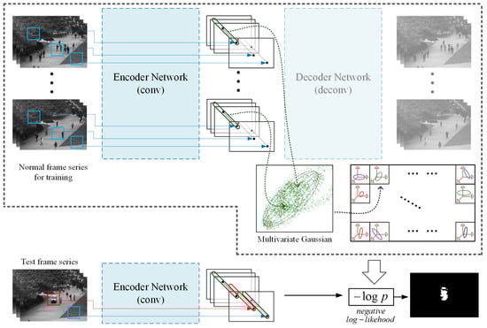
Figure 1.
Appearance and motion representations of each receptive field are learned by our convolutional variational auto-encoder (VAE) first. Then for each receptive field of the scene, a multivariate Gaussian is modelled to fit the feature vector during training. At test time, the negative log-likelihood of each receptive field is computed using the corresponding multivariate Gaussian.
In our work, a series of frames instead of a single frame are used as the input and each training frame series consists of several normal frames. Then, a convolution based variational auto-encoder is constructed to learn appearance and motion representations of the normal frame series, as a method of semi-supervised learning. According to the convolutional neural network, the feature vector at each location of the feature map, which is the output of the encoder, is considered as the appearance and motion representations of its corresponding receptive field. Then, for the feature vectors of the receptive fields at the same location in all inputs, a multivariate Gaussian is modelled to fit them so that each receptive field at different locations has the own corresponding Gaussian model. Once the encoder network and the Gaussian models are trained, receptive fields of low probability under the corresponding Gaussian are considered abnormalities. Given a test frame series, the feature vector of each receptive field is extraced by the encoder network, and its negative log-likelihood under its own Gaussian is computed. In the following we describe the proposed system in detail.
3.2. Convolutional VAE Architecture and Feature Extraction
The network architecture of our convolution based variational auto-encoder (VAE) [18] is shown in Figure 2. In our work, a frame sequence is represented by a set of regional appearance and motion feature vectors, which are extracted densely from the corresponding receptive fields by the following convolution based VAE.
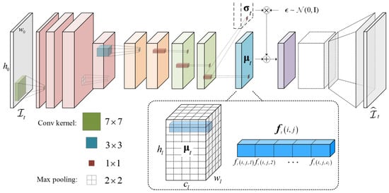
Figure 2.
The network architecture of the proposed convolution-based VAE. Three blocks with different convolution kernels marked green, blue, and red constitute the encoder. The mean map output by the encoder is defined as the feature matrix that consists of the feature vector from each position.
Taking both appearance and motion patterns into account, a series of frames is used as the input. Specifically, suppose we have T frames in the training dataset and all the frames are free of abnormal events, the pixel-wise average of frame and previous frame denoted by and the same as the frame , with the next frame denoted by , are used,
where is the tth frame in the video. Thus, the sequence is used as as a multichannel image to detect anomalies in frame and the sequence set is .
In the feature description step, our convolution based VAE has a deep fully convolutional architecture that contains an encoder network and a decoder network. The encoder can be divided into three blocks according to the size of the convolution kernel. The first block consists of three convolutional layers with the same kernel size and the same stride , and a max pooling layer with a kernel and stride. The second block has two convolutional layers with kernel size and stride . The third block contains three convolutional layers with the same kernel size and stride . Then according to the VAE, which assumes the posterior distribution of each latent variable takes on an approximate Gaussian form, the encoder outputs a mean map and a standard deviation map , which are the parameters for the posterior distributions of the latent variables. The reparameterization trick is used to generate samples from the posterior distributions of the latent variables, , where and ⊗ as an element-wise product. Next, the samples are pushed into the following decoder network. Compare with the encoder, the followed decoder has the same reversed structure with the deconvolutional layers instead of the convolutional layers.
Specifically, for the tth sequence with the resolution , our encoder network outputs a mean tensor and a standard deviation tensor , where , h, w are the height and width of the tensor map, c is the number of channels, and l is the layer of the network.
Following the work in VAE, the loss function is mainly comprised of two parts. Here we give the equations used for the calculation as follows. The first part could be considered as the reconstruction loss to make the generated frame series close to the original series , thus the loss function can be defined as follows:
In addition, as we assume the distribution of each feature representation that described by a mean map and a standard deviation map takes on an approximate Gaussian form with an approximate diagonal covariance, the second part is the Kullback–Leibler (KL) divergence, which measures the difference between two probability distributions.
Specifically, the KL divergence can be computed and differentiated without estimation:
where is the total number of the pixels in the mean tensor (also the standard deviation tensor). Finally, the total loss function is as follows.
In the training processing, Adam [43] based Stochastic Gradient Descent method is used for parameter optimization and the learning rate is set to 0.0001. As a fully convolutional network, the resolutions of input and output are the same. Consequently, there is no need to crop or resize the input video frames.
Different from ordinary auto-encoder, the variational auto-encoder aims to learn the posterior distributions of feature representations, in the form of parameters mean and standard deviation . From the view of numerical simulation, the mean can be treated as a statistical representation of the input data and the standard deviation as a noise intensity regulator. Therefore, for the input series , we define the mean tensor from the encoder as the feature representation of the appearance and motion patterns. Suppose we have the mean tensor with size from the encoder at the lth layer, the feature representation is considered to consist of feature vectors with dimensions. Specifically, for each position , where , the feature vectors can be written as:
According to the architecture of the conventional neural network, each feature vector is derived from a specific receptive field, which is a sub-region of the original sequence . In other words, instead of cropping the sequence into patches and extracting the features one by one, we divide the sequence into overlapping patches containing appearance and motion information densely and extract features , from all the receptive fields at one time.
In general, the features learned by our convolutional VAE are the further statistical representations of that learned by an ordinary convolutional auto-encoder, which means our features can represent the appearance and motion patterns that the receptive fields belong to rather than just some specific receptive fields samples. On the other hand, according to the assumption and the corresponding constraint condition of VAE, the elements of our feature vector tend to be independent and decoupled, comparing with the feature learned by the conventional auto-encoder.
3.3. Anomaly Detection and Localization
In the training phase, all the frames and the frame series are free of abnormal events and thus the features extraced from them are considered as normal features. As mentioned above, the appearance and motion patterns in each receptive field of a video sequence are represented using a feature vector from the encoder of our fully convolutional network, where is corresponding location on the feature map and .
To model all the normal features that form the training frame series and to check whether the upcoming features are abnormal or not, Gaussians are constructed to fit the normal features. Different from other works that used only one model to fit all the feature vectors, we construct different Gaussian models to fit the normal feature vectors extracted from each receptive field. Besides this, considering the residual correlation among the elements of a feature vector, the multivariate Gaussian is adopted to improve the accuracy. Specifically, for each location of the feature tensor, an exclusive multivariate Gaussian model with variables is fitted to all normal feature vectors extracted from all frame series , where T is the number of the normal frames:
where is the mean vector, is the covariance matrix and is the dimension of . Therefore, we define these Gaussian models as our reference models for normal appearance and motion patterns.
In the anomaly detection phase, input sequences are pushed into the encoder network first. Then feature vectors are extracted by the encoder network. These feature vectors are varified by the corresponding Gaussian model . Observations of low probability under these Gaussian model are declared anomalies. In our work, the log-likelihood of a feature vector under the Gaussian model is used to measure the anomaly so that the abnormality map at location is the negative log-likelihood of the feature vector :
In addition, the location of the anomalies can be mapped from the feature maps layer to the original frame. According to the convolution and pooling processes of CNN, all the feature vectors are extraced from the corresponding receptive fields that overlap each other in sequence for considering the tth frame. As the kernel of each convolution and pooling processes has the fixed size, therefore, the abnormality of each receptive field in the original tth frame can be backward mapped by the abnormality at each location in the abnormality map. For the regions where the receptive fields overlap in the original frame, an averaging operation is used to calculate the final anomaly score.
4. Experimental Results and Comparisons
We evaluate the performance of the proposed method mainly on the large scene surveillance dataset: UCSD Anomaly Detection Dataset (http://www.svcl.ucsd.edu/projects/anomaly/dataset.htm). The UCSD Anomaly Detection Dataset was acquired with a stationary camera mounted at an elevation, overlooking pedestrian walkways. The crowd density in the walkways was variable, ranging from sparse to very crowded. The UCSD dataset includes two subsets: Ped1 and Ped2. Both contain training set and testing set. Specifically, Ped1 contains 34 training video sequences and 36 testing video sequences. The frame resolution is pixels. In Ped1, people walk towards and away from the camera so that the foreshortening effects occur; Ped2 contains 16 training video sequences and 12 testing video sequences with pedestrian movement parallel to the camera plane. The frame resolution is pixels. All frames in the training set are normal and contain only pedestrians. In addition to normal frames, the testing set contains abnormal frames with bikers, skaters, small carts or people walking in the grass as anomalies. We also make an additional experiment on the ShanghaiTech Campus dataset (https://svip-lab.github.io/dataset/campus_dataset.html) to evaluate our method. The ShanghaiTech Campus dataset includes 13 scenes and each scenes are of complex light conditions and camera angles. Each color frame resolution is pixels. The same as the UCSD dataset, all the videos for training are normal and contain only pedestrians and the testing frames for each scene contains abnormal events, such as bikers, people running and fighting.
All experiments are carried out on a dedicated GPU server with Intel Xeon E5-2620 CPU running at 2.1 GHz, 128 GB of RAM, a Nvidia TITANX GPU and running Ubuntu Mate 16.04. We use the Pytorch library, which is an open-source machine learning library for Python, to implement our anomaly detection architecture.
4.1. Visualization of the Feature Distribution
Given a sequence as input, our VAE outputs the feature map in the size of , which means we extract a c-dimension feature vector at each location . To observe the distribution of the feature vectors, we set the feature dimension c to 3 as an example and select a fixed location . Then we can scatter the feature vectors , which are extracted from the same receptive field of both training and testing sequence sets, in a three-dimensional grid as follows.
As shown in Figure 3, all the feature vectors extracted from the same receptive field of the input series are plotted as scatter points in the 3-dimensional coordinate system. The distribution of both training and testing scatter points is almost a 3D fusiform shape, which is a typical shape of the multivariate Gaussian distribution. Moreover, the contours of the projection on the three planes also indicate that the distribution of the scatter points is Gaussian. Then we examine the relationship between the receptive patches and the feature points and take three from testing samples as examples. The feature vectors that near the center come from the normal samples (the pedestrian and background) and some similar samples of anomalies (the cyclist). The points that far from the center come from the anomaly samples (the car). This distribution trend indicates that the fitting the feature vectors by Gaussian is feasible.
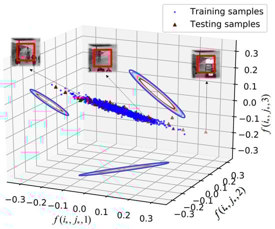
Figure 3.
The distribution of the receptive field from the same position in the three-dimensional feature space.
4.2. Qualitative and Quantitative Results
For the UCSD Anomaly Detection Dataset, the receiver operating characteristic (ROC) curves, the equal error rate (EER), and the area under curve (AUC) are used to compare our results with state-of-art methods. Two measures at frame level and pixel level are used, which are introduced in [32] and widely used in later works. In essence, both of the two measures focus on the anomaly of a frame. For frame level evaluation, a frame is considered an anomaly if at least one pixel is recognized as an anomaly, whether the recognition result is correct or wrong. For pixel level evaluation, a frame is considered to contain anomalies if at least of anomaly ground truth are covered by the regions that are detected by the algorithm. In other words, the anomaly of a frame can be determined only when the anomaly object in it is accurately located.
We compare our anomaly detection method with several methods. Specifically, we consider some classical methods that are widely cited as the baselines for the UCSD Anomaly Detection Dataset, which contains the sparse combination learning framework (SCLF) in [36], the mixture of probabilistic principal component analyzers (MPPCA) approach in [31], the social force model (SF) in [44], and their extension (SF+MPPCA) in [32], mixture of dynamic texture (MDT) in [32] and Adam method in [30]. In addition to these classical baselines, we also consider two state-of-the-art methods, the sparse reconstruction method in [37] and the Appearance and Motion DeepNet (AMDN) method in [21].
Figure 4 and Figure 5 plot the ROC curves of the various algorithms for comparison. By varying the threshold parameter, we can obtain a series anomaly detection results and their corresponding false positive rates (FPR) and true positive rates (TPR). Thus, the ROC curve can be plotted by the series of coordinate points composed of FPRs and TPRs. The ROC curves of the baseline methods are taken from the original papers (when available). From the frame-level evaluation results, it shows that our method outperforms most previous methods and yields competitive performance comparing with two state-of-the-art methods AMDN [21] and Sparse reconstruction [37]. Moreover, from the pixel-level evaluation results, which reflect the accuracy of anomaly localization, our method outperforms all the competing approaches.
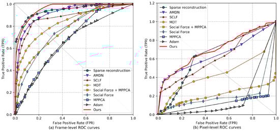
Figure 4.
Receiver operating characteristic (ROC) comparisons of different methods on Ped1 dataset. (a) Plots the frame-level ROC curves and (b) plots the pixel-level ROC curves.
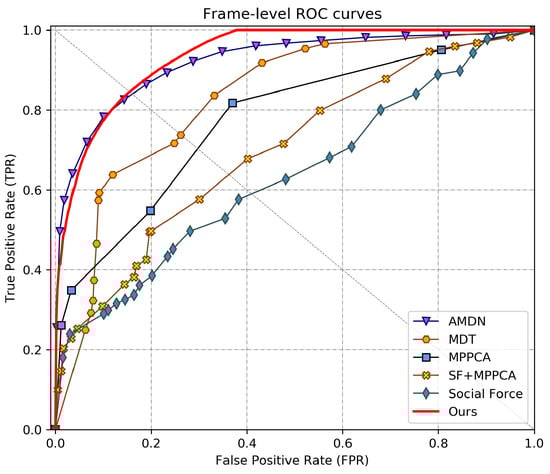
Figure 5.
ROC comparison of different methods on Ped2 dataset for frame-level.
In addition to the ROC curves, the evaluation criteria also include two numerical indices, AUC and EER in frame-level and pixel-level, and the results are presented in Figure 6 and Table 1. It is noted that the lower EER and higher AUC indicate better performance. Comparing with the sparse reconstruction methods [37], which achieved an outstanding result without using deep learning methods, our method achieves only about 1% AUC increase and the same EER for frame-level detection. However, for pixel-level detection, our method achieves about 6% AUC increase, which means our methods locates the anomalies more accurately. Compared with other AMDN methods [21], which had superior performance by using the deep neural network based auto-encoders to learn feature representations, our method achieves about 3% AUC increases, 4% EER reduction for Ped1 frame-level detection and about 1.5% AUC increases, 2% EER reduction for Ped2 frame-level detection. For pixel-level detection, our method achieves a 3% AUC increase.
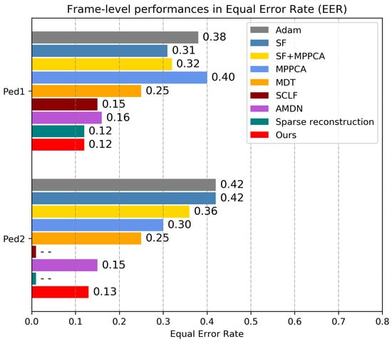
Figure 6.
Equal error rate (EER) comparison of frame-level performance with different methods. Note that the performances of the sparse combination learning framework (SCLF) [36] and the sparse reconstruction [37] on Ped2 dataset are not available.

Table 1.
Area under curve (AUC) comparison with the state of art methods.
We report some examples of anomaly detected with our method on the UCSD dataset in Figure 7. Our detection results are marked with red color and the groundtruth manually labeled are marked with green color. Besides the obvious single anomaly, such as the bikers and the vehicles in (a), (b), (f), and (g), our method also works well in other complex scenes. In the scenes (c), (h), and (i), two abnormal events occur simultaneously. In (d), as our method can learn the appearance and motion feature representations, the skater that is almost the same as the pedestrian can also be detected. In (e) and (j), the anomalies are surrounded by normal pedestrians.
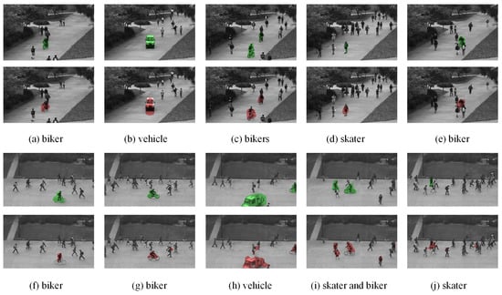
Figure 7.
Examples of anomaly detection results on Ped1 (top) and Ped2 (bottom) sequences. The detection results are marked with red color and the groundtruth are with green color.
Some failure cases that impede the performance of our method are reported in Figure 8. In Figure 8a, a man is walking along the street with nothing, but a box suddenly appears in his hand at the end of the sequence. Then our system wrongly detects him as an anomaly. In Ped1 sequence (b), a biker is almost the same as a pedestrian in some special angles, which causes our system to fail to detect it. In Ped2 sequence (c), part of the biker that appears at the bottom of the frame is correctly detected as an anomaly. However, for the biker that appears in the middle of the frame, our system misses it since the biker is similar to the grass background and the edge of the bike is too tiny to activate our system.
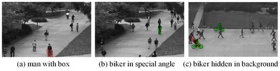
Figure 8.
Examples of failure results on Ped1 and Ped2 sequences. The detection results are marked with red color and the groundtruth are with green color.
In addition to UCSD Anomaly Detection Dataset, we also evaluate the performance of the proposed methods on the new colord surveillance dataset: ShanghaiTech Campus dataset. We compare our anomaly detection method with two methods, Conv-AE [40] and FFP [6], since the dataset has not been widely used. The Area Under Curve (AUC) is cumulated to a scalar for performance evaluation. Following the work in [6], we leverage frame-level AUC for performance evaluation.
The AUC of these two methods are taken from FFP [6] and listed with our method together in Table 2. For the 13 different scenes in the dataset, we trained their own models instead of only one model on all 13 scenes altogether like FFP did, because the definition of anomaly is different in these different scenes. We can see that our method outperforms the other two methods, which demonstrates the effectiveness of our method for colored scenes.
Table 2.
AUC comparison on the ShanghaiTech dataset.
4.3. Run-Time Analysis
We compare the running time of our method with the other approaches on UCSD dataset. Different image resolutions affect the time required to process each frame. Specifically, the resolutions are for the UCSD Ped1 dataset and for the UCSD Ped2 dataset. Table 3 reports the average running time of each frame during the test phase. Since the original implementations of the other methods are not publicly avilable, we report the running times taken from [21,36], specifying the working environment. Inevitably, the improvement in terms of accuracy obtained with deep neural network comes at a price of an increased computational cost. Compared with AMDN [21], which also adopted a deep architecture, the computational speed of our method is faster. The main reason is that our method benefits from fully convolutional neural network that can extract the feature representations of all the receptive fields in the input frames at one time, and AMDN crops the input into patches and the same feature extraction process is repeated among these patches. As shown in Table 3, with a GPU, our method has great time efficiency in terms of anomaly detection.
Table 3.
Comparison of different methods in terms of running time (seconds per frame).
5. Conclusions
In this paper, we introduce a novel unsupervised learning approach for a video anomaly detection system based on convolutional auto-encoder architectures. We focus on the anomalies that occur in outdoor scenes, considering the challenging publicly available UCSD anomaly detection datasets. The fundamental advantage of our approach is the use of a variational convolutional auto-encoder. On the one hand, our approach can extract features independent of the prior knowledge of hand-crafted features (the input of our detection system are raw pixels) and dispenses with any object-level analysis, like object detection and tracking. On the other hand, we omit the process of cropping the input into patches by the convolution principle of the convolutional neural network, which makes our framework simple and clear. We demonstrate the effectiveness and robustness of the proposed approach, showing competitive performance to existing methods.
In fact, the approcah we present for the anomaly detection system can be viewed as a baseline of using a variational auto-encoder to detect anomalies in surveillance video. Further research directions will include jointing the input with richer temporal and contextual information and combining the feature extraction with the final anomaly decision. Besides, we can learn from the deep neural network frameworks for object detection and classification tasks to design more sophisticated frameworks, in order to represent the multiple patterns from the input video.
Author Contributions
All the authors made significant contributions to this work. Conceptualization, M.X. and D.C.; methodology, M.X. and D.C.; validation, M.X., X.Y. and C.W.; formal analysis, M.X. and X.Y.; investigation, M.X.; writing—original draft preparation, M.X.; writing—review and editing, M.X., D.C. and C.W.; supervision, C.W. and Y.J.
Funding
This research was funded by National Natural Science Foundation of China under Grant 61701101, U1713216 and U1613214, National Key R&D Program of China under Grant 2017YFC0821402, National Key Robot Project under Grant 2017YFB1300900 and 2017YFB1301103, Fundamental Research Fund for the Central Universities of China N172603001, N172604004, N172604002 and N181602014.
Acknowledgments
We are thankful to anonymous editor and reviewers for their valuable comments and kind suggestions in early versions of this article.
Conflicts of Interest
The authors declare no conflict of interest.
References
- Ye, R.; Li, X. Collective representation for abnormal event detection. J. Comput. Sci. Technol. 2017, 32, 470–479. [Google Scholar] [CrossRef]
- Sun, Q.; Liu, H.; Harada, T. Online growing neural gas for anomaly detection in changing surveillance scenes. Pattern Recognit. 2017, 64, 187–201. [Google Scholar] [CrossRef]
- de Almeida, I.R.; Cassol, V.J.; Badler, N.I.; Musse, S.R.; Jung, C.R. Detection of global and local motion changes in human crowds. IEEE Trans. Circuits Syst. Video Technol. 2017, 27, 603–612. [Google Scholar] [CrossRef]
- Xiao, T.; Zhang, C.; Zha, H. Learning to detect anomalies in surveillance video. IEEE Signal Process. Lett. 2015, 22, 1477–1481. [Google Scholar] [CrossRef]
- Biswas, S.; Gupta, V. Abnormality detection in crowd videos by tracking sparse components. Mach. Vis. Appl. 2017, 28, 35–48. [Google Scholar] [CrossRef]
- Liu, W.; Luo, W.; Lian, D.; Gao, S. Future frame prediction for anomaly detection—A new baseline. In Proceedings of the 2018 IEEE/CVF Conference on Computer Vision and Pattern Recognition, Salt Lake City, UT, USA, 18–22 June 2018; pp. 6536–6545. [Google Scholar] [CrossRef]
- Afiq, A.A.; Zakariya, M.A.; Saad, M.N.; Nurfarzana, A.A.; Khir, M.H.M.; Fadzil, A.F.; Jale, A.; Gunawan, W.; Izuddin, Z.A.A.; Faizari, M. A review on classifying abnormal behavior in crowd scene. J. Vis. Commun. Image Represent. 2019, 58, 285–303. [Google Scholar] [CrossRef]
- Reddy, V.; Sanderson, C.; Lovell, B.C. Improved anomaly detection in crowded scenes via cell-based analysis of foreground speed, size and texture. In Proceedings of the CVPR 2011 WORKSHOPS, Colorado Springs, CO, USA, 20–25 June 2011; pp. 55–61. [Google Scholar] [CrossRef]
- Bertini, M.; Del Bimbo, A.; Seidenari, L. Multi-scale and real-time non-parametric approach for anomaly detection and localization. Comput. Vis. Image Underst. 2012, 116, 320–329. [Google Scholar] [CrossRef]
- Biswas, S.; Babu, R.V. Anomaly detection via short local trajectories. Neurocomputing 2017, 242, 63–72. [Google Scholar] [CrossRef]
- Saligrama, V.; Chen, Z. Video anomaly detection based on local statistical aggregates. In Proceedings of the 2012 IEEE Conference on Computer Vision and Pattern Recognition, Providence, RI, USA, 16–21 June 2012; pp. 2112–2119. [Google Scholar] [CrossRef]
- Hugo Mora Colque, R.V.; Caetano, C.; Lustosa de Andrade, M.T.; Schwartz, W.R. Histograms of optical flow orientation and magnitude and entropy to detect anomalous events in videos. IEEE Trans. Circuits Syst. Video Technol. 2017, 27, 673–682. [Google Scholar] [CrossRef]
- Zhang, Y.; Lu, H.; Zhang, L.; Ruan, X.; Sakai, S. Video anomaly detection based on locality sensitive hashing filters. Pattern Recognit. 2016, 59, 302–311. [Google Scholar] [CrossRef]
- Krizhevsky, A.; Sutskever, I.; Hinton, G.E. ImageNet classification with deep convolutional neural networks. Commun. Acm 2017, 60, 84–90. [Google Scholar] [CrossRef]
- Girshick, R.; Donahue, J.; Darrell, T.; Malik, J. Rich feature hierarchies for accurate object detection and semantic segmentation. In Proceedings of the 2014 IEEE Conference on Computer Vision and Pattern Recognition, Columbus, OH, USA, 23–28 June 2014; pp. 580–587. [Google Scholar] [CrossRef]
- Vincent, P.; Larochelle, H.; Bengio, Y.; Manzagol, P.A. Extracting and composing robust features with denoising autoencoders. In Proceedings of the 25th International Conference on Machine Learning, Helsinki, Finland, 5–9 July 2008; pp. 1096–1103. [Google Scholar] [CrossRef]
- Vincent, P.; Larochelle, H.; Lajoie, I.; Bengio, Y.; Manzagol, P.A. Stacked denoising autoencoders: Learning useful representations in a deep network with a local denoising criterion. J. Mach. Learn. Res. 2010, 11, 3371–3408. [Google Scholar]
- Kingma, D.P.; Welling, M. Auto-encoding variational bayes. arXiv 2013, arXiv:1312.6114. [Google Scholar]
- Long, J.; Shelhamer, E.; Darrell, T. Fully convolutional networks for semantic segmentation. In Proceedings of the 2015 IEEE Conference on Computer Vision and Pattern Recognition, Boston, MA, USA, 7–12 June 2015; pp. 3431–3440. [Google Scholar]
- Ribeiro, M.; Lazzaretti, A.E.; Lopes, H.S. A study of deep convolutional auto-encoders for anomaly detection in videos. Pattern Recognit. Lett. 2018, 105, 13–22. [Google Scholar] [CrossRef]
- Xu, D.; Yan, Y.; Ricci, E.; Sebe, N. Detecting anomalous events in videos by learning deep representations of appearance and motion. Comput. Vis. Image Underst. 2017, 156, 117–127. [Google Scholar] [CrossRef]
- Sabokrou, M.; Fayyaz, M.; Fathy, M.; Moayed, Z.; Klette, R. Deep-anomaly: Fully convolutional neural network for fast anomaly detection in crowded scenes. Comput. Vis. Image Underst. 2018, 172, 88–97. [Google Scholar] [CrossRef]
- Wu, S.; Moore, B.E.; Shah, M. Chaotic invariants of Lagrangian particle trajectories for anomaly detection in crowded scenes. In Proceedings of the 2010 IEEE Computer Society Conference on Computer Vision and Pattern Recognition, San Francisco, CA, USA, 13–18 June 2010; pp. 2054–2060. [Google Scholar] [CrossRef]
- Tung, F.; Zelek, J.S.; Clausi, D.A. Goal-based trajectory analysis for unusual behaviour detection in intelligent surveillance. Image Vis. Comput. 2011, 29, 230–240. [Google Scholar] [CrossRef]
- Kumar, D.; Bezdek, J.C.; Rajasegarar, S.; Leckie, C.; Palaniswami, M. A visual-numeric approach to clustering and anomaly detection for trajectory data. Vis. Comput. 2017, 33, 265–281. [Google Scholar] [CrossRef]
- Dalal, N.; Triggs, B. Histograms of oriented gradients for human detection. In Proceedings of the 2005 IEEE Computer Society Conference on Computer Vision and Pattern Recognition (CVPR’05), San Diego, CA, USA, 20–25 June 2005; Volume 1, pp. 886–893. [Google Scholar] [CrossRef]
- Dalal, N.; Triggs, B.; Schmid, C. Human detection using oriented histograms of flow and appearance. In Computer Vision ECCV 2006; Springer: Berlin/Heidelberg, Germany, 2006; pp. 428–441. [Google Scholar]
- Kratz, L.; Nishino, K. Anomaly detection in extremely crowded scenes using spatio-temporal motion pattern models. In Proceedings of the 2009 IEEE Conference on Computer Vision and Pattern Recognition, Miami, FL, USA, 20–25 June 2009; pp. 1446–1453. [Google Scholar] [CrossRef]
- Xu, D.; Song, R.; Wu, X.; Li, N.; Feng, W.; Qian, H. Video anomaly detection based on a hierarchical activity discovery within spatio-temporal contexts. Neurocomputing 2014, 143, 144–152. [Google Scholar] [CrossRef]
- Adam, A.; Rivlin, E.; Shimshoni, I.; Reinitz, D. Robust real-time unusual event detection using multiple fixed-location monitors. IEEE Trans. Pattern Anal. Mach. Intell. 2008, 30, 555–560. [Google Scholar] [CrossRef]
- Kim, J.; Grauman, K. Observe locally, infer globally: A space-time MRF for detecting abnormal activities with incremental updates. In Proceedings of the 2009 IEEE Conference on Computer Vision and Pattern Recognition, Miami, FL, USA, 20–25 June 2009; pp. 2921–2928. [Google Scholar] [CrossRef]
- Mahadevan, V.; Li, W.; Bhalodia, V.; Vasconcelos, N. Anomaly detection in crowded scenes. In Proceedings of the 2010 IEEE Computer Society Conference on Computer Vision and Pattern Recognition, San Francisco, CA, USA, 13–18 June 2010; pp. 1975–1981. [Google Scholar] [CrossRef]
- Li, W.; Mahadevan, V.; Vasconcelos, N. Anomaly detection and localization in crowded scenes. IEEE Trans. Pattern Anal. Mach. Intell. 2014, 36, 18–32. [Google Scholar] [CrossRef] [PubMed]
- Feng, Y.; Yuan, Y.; Lu, X. Learning deep event models for crowd anomaly detection. Neurocomputing 2017, 219, 548–556. [Google Scholar] [CrossRef]
- Cong, Y.; Yuan, J.; Liu, J. Sparse reconstruction cost for abnormal event detection. In Proceedings of the CVPR 2011, Colorado Springs, CO, USA, 20–25 June 2011; pp. 3449–3456. [Google Scholar] [CrossRef]
- Lu, C.; Shi, J.; Jia, J. Abnormal event detection at 150 FPS in MATLAB. In Proceedings of the 2013 IEEE International Conference on Computer Vision, Sydney, NSW, Australia, 1–8 December 2013; pp. 2720–2727. [Google Scholar] [CrossRef]
- Yu, B.; Liu, Y.; Sun, Q. A content-adaptively sparse reconstruction method for abnormal events detection with low-rank property. IEEE Trans. Syst. Man Cybern. Syst. 2017, 47, 704–716. [Google Scholar] [CrossRef]
- Sabokrou, M.; Fathy, M.; Hoseini, M.; Klette, R. Real-time anomaly detection and localization in crowded scenes. In Proceedings of the 2015 IEEE Conference on Computer Vision and Pattern Recognition Workshops (CVPRW), Boston, MA, USA, 7–12 June 2015; pp. 56–62. [Google Scholar] [CrossRef]
- Revathi, A.R.; Kumar, D. An efficient system for anomaly detection using deep learning classifier. Signal Image Video Process. 2017, 11, 291–299. [Google Scholar] [CrossRef]
- Hasan, M.; Choi, J.; Neumann, J.; Roy-Chowdhury, A.K.; Davis, L.S. Learning temporal regularity in video sequences. In Proceedings of the 2016 IEEE Conference on Computer Vision and Pattern Recognition, Las Vegas, NV, USA, 27–30 June 2016; pp. 733–742. [Google Scholar] [CrossRef]
- Narasimhan, M.G.; Kamath, S.S. Dynamic video anomaly detection and localization using sparse denoising autoencoders. Multimed. Tools Appl. 2018, 77, 13173–13195. [Google Scholar] [CrossRef]
- Sabokrou, M.; Fayyaz, M.; Fathy, M.; Klette, R. Deep-cascade: Cascading 3D deep neural networks for nast anomaly detection and localization in crowded scenes. IEEE Trans. Image Process. 2017, 26, 1992–2004. [Google Scholar] [CrossRef] [PubMed]
- Kingma, D.P.; Ba, J. Adam: A method for stochastic optimization. arXiv 2014, arXiv:1412.6980. [Google Scholar]
- Mehran, R.; Oyama, A.; Shah, M. Abnormal crowd behavior detection using social force model. In Proceedings of the 2009 IEEE Conference on Computer Vision and Pattern Recognition, Miami, FL, USA, 20–25 June 2009; pp. 935–942. [Google Scholar] [CrossRef]
© 2019 by the authors. Licensee MDPI, Basel, Switzerland. This article is an open access article distributed under the terms and conditions of the Creative Commons Attribution (CC BY) license (http://creativecommons.org/licenses/by/4.0/).