Gait Classification Using Mahalanobis–Taguchi System for Health Monitoring Systems Following Anterior Cruciate Ligament Reconstruction

Featured Application

This novel method can be implemented by orthopaedic doctors or physiotherapists to provide a clinical assessment of their Anterior Cruciate Ligament Reconstruction patients with more objective, efficient and effective way.

Abstract

In this paper, a gait patterns classification system is proposed, which is based on Mahalanobis–Taguchi System (MTS). The classification of gait patterns is necessary in order to ascertain the rehab outcome among anterior cruciate ligament reconstruction (ACLR) patients. (1) Background: One of the most critical discussion about when ACLR patients should return to work (RTW). The objective was to use Mahalanobis distance (MD) to classify between the gait patterns of the control and ACLR groups, while the Taguchi Method (TM) was employed to choose the useful features. Moreover, MD was also utilised to ascertain whether the ACLR group approaching RTW. The combination of these two methods is called as Mahalanobis-Taguchi System (MTS). (2) Methods: This study compared the gait of 15 control subjects to a group of 10 subjects with laboratory. Later, the data were analysed using MTS. The analysis was based on 11 spatiotemporal parameters. (3) Results: The results showed that gait deviations can be identified successfully, while the ACLR can be classified with higher precision by MTS. The MDs of the healthy group ranged from 0.560 to 1.180, while the MDs of the ACLR group ranged from 2.308 to 1509.811. Out of the 11 spatiotemporal parameters analysed, only eight parameters were considered as useful features. (4) Conclusions: These results indicate that MTS can effectively detect the ACLR recovery progress with reduced number of useful features. MTS enabled doctors or physiotherapists to provide a clinical assessment of their patients with more objective way.

1. Introduction

The most frequently executed orthopaedic surgery is anterior cruciate ligament reconstruction (ACLR) [1,2]. Modern ACLR techniques allow steady ligament reconstruction in nearly all cases; however, the outcome of ACLR rehabilitation is not uniformly excellent [3]. At present, one of the most significant discussions regarding ACLR is the actual degree of recovery. According to Groot, Jonkers, Kievit, Kuijer, and Hoozemans, (2017) the purpose of ACLR and rehabilitation is to allow return to work. Recent studies provide comprehensive information about the predictive factors for return to work involving different activities [4,5,6,7,8]. The patient’s ability to return to physical activity following ACLR is dependent on various factors such as the patient’s characteristics (e.g., gender or age) [9,10,11], results of the operation (e.g., damage quality or joint flexibility) [6,11], knee function prior to the ACLR (e.g., muscle power or flexibility) [5,12,13], exercise level before ACLR (e.g., physical activity or level of Tegner activity) [14,15], and emotional aspects (e.g., self-confidence or inspiration) [16,17].

In our review, we found no significant exiting research that focussed on patients’ return to work (RTW) after ACLR using an analytical strategy. Taguchi [18] demonstrated that the Mahalanobis distance (MD) can be used to distinguish the pattern of a specific group, which is similar to the procedure used by healthcare providers to determine if a person has a specific sort of disorder [19,20,21]. The MD is a space measurement based on correlations between variables (attributes) where distinct patterns can be realised and analysed in regard to a reference evaluation. Mahalanobis Distance (MD) is a statistical tool, which is widely used to differentiate pattern of a certain group from other groups [19,21,22,23].

This study aims to method of ACLR analysis that can predict RTW according to spatiotemporal data. Our proposed method uses the MD to differentiate the routine of ACLR; based on signal-to-noise ratios (S/N ratios) and orthogonal arrays (OAs), useful features can be identified [19,21,22,24]. Associated studies, such as MD, are explained in Section 2. In Section 3, the suggested strategy presented and a case study utilising the suggested strategy demonstrated in Section 4. Some discussion is provided in Section 5 and Section 6, followed by our conclusions in Section 7.

2. Related Study

2.1. ACLR

Anterior cruciate ligament (ACL) injury is one of the most frequent injuries in sport traumatology and ligament instability [25]. In the United States, approximately 90% of accidental ACL injuries are handled by ligament reconstruction clinical procedures. Even though the medium- and long-term results are not as good as anticipated by the orthopaedic community, it is thought to be the best option available [26,27]. Almost people with anterior cruciate ligament damage will experience pain, functional constraints, and radiographic signs of osteoarthritis from the wounded knee within 12–20 years of the injury [28,29,30].

In a group evaluation, Paterno et al. reported that the incidence of knee sprains in the first year after ACL injury is 15 times larger than it was before [31]. They also indicate that after ACL injury and reconstruction, the prevalence of accidental injuries at the contralateral knee is higher than expected for uninjured recreational sportspersons [31]. The fact that defects are not restored by the rehabilitation process can be explained by the high prevalence of recurring sprains after ACLR [32,33]. Biomechanical studies have demonstrated that after two years of rehabilitation injured people tend to adapt their lower limb motion routine for many tasks [26,27]. However, we were unable to find a consensus in the literature regarding the time required before sports activities are permitted. A methodical review by Barber-Westin and Noyes found that return to sports should be based on practice parameters such as ligament laxity on examination, muscle healing compared to the contralateral limb, and a few particular operational assessments [34]. Nevertheless, these conditions are subjective and do not include the identification of possible dangers such as potential comorbidities or re-injuries; therefore, methods that quantify residual deficits are likely to be preferable [34].

Even after ACLR and recovery, changes in gait patterns can be recognised [35]. It has been proven that ACLR subjects have an inclination to pose altered knee angles during gait, even 12 months after the operation [36]. With no changes in the sagittal plane, the major altered variables were connected to increased adduction and rotation of the knee. These factors alter the angle of the frontal and transverse planes of the knee during gait and have been related to premature knee osteoarthritis [37]. For clinical training, the assessment of complex motions is frequently limited by the large expense of instruments. However, spatiotemporal gait parameters are gait performance indicators that require relatively low-cost equipment [2]. Therefore, we aim to develop a predictive technique for ACLR diagnosis based on the spatiotemporal parameters of ACLR groups and to classify the status of normality [19,22,24,38]. The recommended strategy utilises the MD to identify significant features and to identify patterns related to ACLR that can be used for the return to work assessments [23,39].

2.2. Mahalanobis–Taguchi System (MTS)

2.2.1. Four Steps in MTS

The data were analysed using the Mahalanobis–Taguchi System (MTS) [40], a combinations of MD and Taguchi strategies. MD is a generalised distance that is useful for identifying similarities between healthy and unhealthy sample sets and a scalar value is used to represent a multivariate system [39]. Taguchi strategies are statistical approaches used to enhance the engineered quality and to make the system more powerful [24,41,42]. There are four steps in a MTS [40]:

Step 0: Identification of assessment criteria and collection of patients’ spatiotemporal data

Step I: Mahalanobis space (MS) creation

Data from the healthy subjects are collected to create the standard data set; their MDs constitute a reference space that is called MS. Their MDs are approximately equal to one. In this study, a feature data set consisting of spatiotemporal data from healthy subjects was used to create the MS. The healthy data set is denoted as H; $h_{ij}$ is the $i\mathrm{th}$ observation on the $j\mathrm{th}$ feature, where $i=1,2,\dots ,m,$ and $j=1,2, \dots , n.$ Then, ${\overline{H}}_j$ and $S_j$ are the mean and standard deviation of the $j$th feature $\left(H_j\right)$, respectively, where $j =1,2, \dots , n$. Each individual feature of each data vector ($H_j$) is normalised by the mean ($\overline{H_j}$) and the standard deviation ($S_j$). Hence, the normalised values are as follows:

$$z_{ij}=\frac{h_{ij}-\overline{H_j}}{S_j} , i=1,2,\dots ,m,j=1,2,\dots ,n$$

(1)

where

$$\overline{H_j}=\frac{1}{m}{\displaystyle \sum }_{i=1}^m{h}_{ij}$$

(2)

and

$$S_j=\sqrt{\frac{{{\displaystyle \sum }}_{i=1}^m{\left(h_{ij}-\overline{H_j}\right)}^2}{m-1}}$$

(3)

The MDs of the healthy dataset are calculated with the following formula:

$$M{D}_i=\frac{1}{n}{z}_i{C}^{-1}{z}_i^T$$

(4)

where $z=\left[z_{i1},z_{i2}\dots ,z_{in}\right], z_i^T$ is the transpose vector and $z_i\mathrm{and} C^{-1}$ is the inverse of the covariance coefficient matrix $C$. We compute $C$ as:

$$C=\frac{1}{m-1}{\displaystyle \sum }_{i=1}^m{z}_i^T{z}_i$$

(5)

Multicollinearity (strong correlations among features) is one issue confronted by MD. Multicollinearities will have a problematic impact within a singular covariance coefficient matrix, resulting in an imprecise inverse of the covariance coefficient matrix, and subsequently an inaccurate MD [43]. MDA may be utilised to address this issue; MDA is MD corresponding to the adjoint matrix of the covariance coefficient matrix,

$$MD{A}_I=\frac{1}{n}{z}_i{C}_{adj}{z}_i^T$$

(6)

where $C_{adj}$ is the adjoint matrix of the covariance coefficient matrix $C$. Since $C^{-1}=C_{adj}/\left|C\right|$, the relationship between MD and MDA is given by,

$$M{D}_i=\frac{1}{\left|C\right|}MD{A}_i$$

(7)

Step II: Validation of MS

Trials of ACLR subjects are selected [19]. The abnormal data set is symbolised as P; $p_{ij}$ is the $ith$ observation of the $j\mathrm{th}$ feature, where $i=1,2,\dots , m,$ and $j=1,2, \dots , n.$ It is normalised by applying the mean and standard deviation of the healthy data set while the MDs are estimated using the feature information and the data’s coefficient matrix. MDs corresponding to ACLRs will be outside of the MS if the MS is appropriately constructed. In other words, the MDs associated with abnormal conditions will have higher values [20,21].

Step III: Identification of useful features

By utilising the OAs and S/N ratios, useful features are selected. In MTS, OAs are used to recognise significant features by decreasing the number feature combinations established initially. The number of features determines the true number of columns in the OA. Two levels of factors are used: Level-1 means that the feature is included, while Level-2 means that the feature is not included. To measure the accuracy of the MS predictions, S/N ratios are used; these are calculated using only the ACLR conditions. The equation for determining the S/N ratio (${\eta }_i$) corresponding to the ith run of the OA is 1

$${\eta }_i=-10\log \left(\frac{1}{t}{\displaystyle \sum }_{j=1}^t\frac{1}{M{D}_j}\right)$$

(8)

where it is the number of ACLR conditions and $M{D}_j$ is the $MD$ of the $j\mathrm{th}$ ACLR condition. By evaluating the ‘gain’ in the S/N ratios, the useful features are identified. Therefore, by using Equation (9) the gain of each feature is computed. Features with positive gain are considered useful.

$$Gain= \overline{S/Nrati{o}_{Level-1}}- \overline{S/Nrati{o}_{Level-2}}$$

(9)

Step IV: Future diagnosis

The MS is rebuilt using the attributes recorded in Step III and the MDs of the monitored products are calculated. The subjects are healthy if the MDs are inside the MS. If the MDs are outside the MS, then the subjects reveal abnormal (ACLR) behaviours. A greater MD indicates a greater deviation between the healthy and ACLR patients [19].

2.2.2. Determine MD Ranges

MD is a distance metric with values ranging from zero to infinity. Greater MD values are of concern from the perspective of ACLR. The primary problem is to find a suitable threshold $T$ that can distinguish between ACLR and healthy patients for medical diagnosis. If $MD \le T$, the patient is healthy. The patient is injured if $MD>T$. Therefore, sensitivity and specificity analysis are employed to determine the MD ranges corresponding to the difference between the ACLR and healthy patients.

3. Proposed Approach

We propose using the MTS to enhance ACLR diagnosis and analysis. This approach can be split into two phases; the first phase uses the MD to distinguish the routine of ACLR and uses OAs and S/N ratios to select important features [19]. The second phase demonstrates how to use the model created in the initial phase. A flow chart describing this strategy is shown in Figure 1. A broader description is given below.

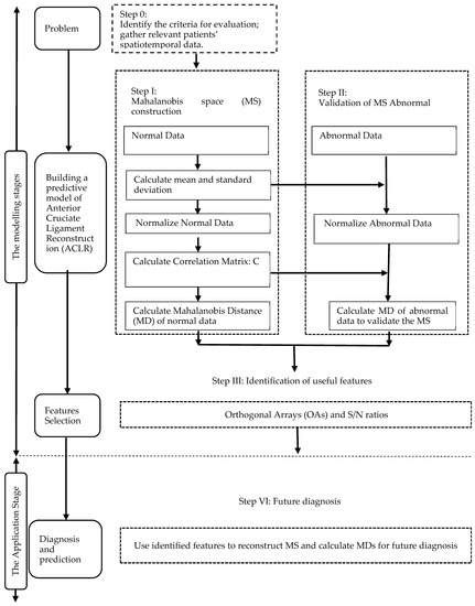
Figure 1. Flow chart of the approach proposed in this study.

3.1. Modelling Stage

There are three steps to developing the model. The first step is to define the issue; this is where we find the spatiotemporal gait parameters. Next, we gather the essential data. We select a ‘normal’ or ‘healthy’ group to construct the MS. Then, we use the information from the healthy group and the spatiotemporal gait parameters to get the Mahalanobis distance MS1, and data from the ACLR group and chosen attributes to get the Mahalanobis distance MS2. Next, we find an appropriate threshold to efficiently distinguish the healthy and ACLR groups. The threshold value is set according to MS1 and MS2 and an effective threshold can improve clinicians’ analytical and forecasting abilities. The final step is attribute selection, where the most vital features are chosen.

3.2. Application Stage

The developed model can be used to forecast ACLR rehabilitation patterns by entering the ACLR data together with the chosen features.

4. Case Study

4.1. Participants

To assess the efficiency of our method, ACLR patients from the Rehab and Physiotherapy Unit of Hospital Tuanku Fauziah at Kangar, Perlis, were considered for this study. Ten patients with a unilateral primary ACLR were chosen for the ACLR group (PG). This group was composed of 10 males. All patients go through similar rehabilitation procedures, beginning passive and active mobilization after the operation. Meanwhile, 15 healthy subjects (HG) were selected for the healthy group with the condition that they had no previous history of lower extremity injuries, surgeries, or neuropathy. The HG consisted of 15 males. The height, age, and weight distribution of the two groups were not significantly (p > 0.05) (Table 1). Ethical approval was granted by the University of Malaysia Perlis, and the participants provided written informed consent.

Table 1. Anthropometric data of the subjects and p-value of relationship between the healthy group (HG) and ACLR group (PG). Values stated as mean ± standard deviation.

Parameter	HG	PG	p-Value
Age (years)	27.73 ± 0.80	25.8 ± 5.41	0.1365
Body mass (kg)	60.22 ± 6.04	71.6 ± 9.66	0.608
Height (cm)	167 ± 5.0	172.0 ± 6.0	0.837

4.2. Procedures

Subjects were instructed to walk seven times on an 8 m walkway. The first two laps were not measured to allow for familiarization with the task and instrumentation. The last five laps were assessed to catch four gait cycles, employing the right limb from the HG and the injured limb from the PG. We compared the ACLR to the right limbs only because most individuals are right leg dominant and we wanted to compare those limbs to a right control limb that is more likely to exhibit ideal and stable knee biomechanics [44,45].

A number of previous studies have compared differences in ACLR limbs to control limbs and the fact that both the right and left control limbs provided similar results and that we observed significant differences between the ACLR and right limbs indicates that we were able to find these differences by concentrating on these limbs [45,46,47].

The trial was conducted in the Motion Lab at the University of Malaysia Perlis. Motion data were collected using five Oqus cameras of a motion capture system (Oqus, Qualisys AB, Gothenburg, Sweden). 36 reflective markers were placed on the joint landmarks and segments of the lower limb as denoted in Figure 2. The cameras were mounted on tripods to capture the static trial of the subject in 2 s at 120 Hz, followed by the walking motion of the subjects. The dynamic trials were captured in 8 s at 480 Hz.

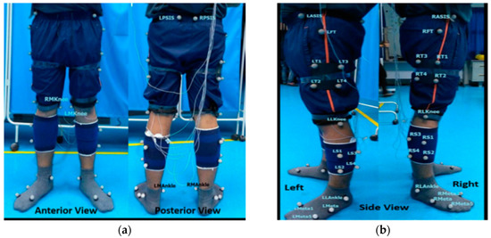
Figure 2. (a) Anterior and posterior views and (b) left and right-side views of marker placement.

Two force plates were reset for the next trial. The vertical ground reaction force was detected by two force plates with dimensions of 400 × 600 mm (Bertec, Worthington, Ohio, OH, USA) while the subject performed several walks at his own pace. At least five success trials were collected and interpreted.

At least five success trials were captured and post-processed using Qualisys Track Manager with a sampling rate of 60 Hz. The 11 spatiotemporal parameters (Table 2) of the trial were generated in Visual 3D Pro v6. This includes variations in the step width, stride speed, swing time, stance time, stride time, step time, step width, stride length and step length.

Table 2. Operational definitions of gait parameters and variables.

	Variables	Operational Definition
Step Length (cm)	X1	Anterior-posterior distance from the heel of one footprint to the heel of the opposite footprint.
Stride Length (cm)	X2	Anterior-posterior distance between the heels of two consecutive footprints of the same foot (left to left, right to right); two steps (e.g., a right step followed by a left step) comprise one stride or one gait cycle.
Step Width (cm)	X3	Lateral distance from the heel centre of one footprint to the line of progression formed by two consecutive footprints of the opposite foot.
Stance Time (s)	X4	The stance phase is the weight bearing portion of each gait cycle beginning at heel contact and ending at toe off of the same foot; stance time is the time elapsed between the initial contact last contact of a single footfall.
Swing Time (s)	X5	The swing begins with toe off and ends with initial contact of the same foot; swing time is the time elapsed between the last contact of the current footfall to the initial contact of the next footfall of the same foot.
Single Support Time (s)	X6	Single support occurs when only one foot is in contact with the ground; single support time is the time elapsed between the last contact of the opposite footfall to the initial contact of the next footfall of the same foot.
Double Support Time (s)	X7	Double support occurs when both feet are in contact with the ground simultaneously; double support time is the sum of the time elapsed during two periods of double support in the gait cycle.
Stance Time (%GC)	X8	Stance time normalised to stride time.
Double Support Time (%GC)	X9	Double support time normalised to stride time.
Gait Speed (m/s)	X10	Calculated by dividing the distance walked by the ambulation time.
Stride Speed (m/s)	X11	Calculated by dividing stride length by the stride time.

Note = %GC = % gait cycle.

4.3. Results

Step I: Construction of MS

After collecting the information (Table 3), we calculated the MD using the formulas given in Section 2.2.1. To compute MD1, we utilised the healthy group data and the 11 features of selection. The 15 healthy subjects were used as the benchmark (healthy) group. The average and standard deviation of every characteristic from the HG were computed (Table 4) and the information from Table 5 was normalised using Equation (1). This normalised information was used to build the correlation matrix and its inverse (see Table 6). Next, the Mahalanobis distances were computed using Equation (4), as presented in Table 7. Likewise, using the inverse correlation matrix (Table 6) generated from the HG data, we computed the Mahalanobis distance for the 10 sets of PG data. The MDs of the HG were approximately equal to one, as shown in Figure 3.

Table 3. Mean and standard deviation (SD) of healthy group (HG) and ACLR group (PG) for all variables.

Parameter	Unit	HG		PG
		Mean	SD	Mean	SD
Step Length	(m)	0.584	0.043	0.562	0.030
Stride Length	(m)	1.161	0.077	1.079	0.197
Step Width	(m)	0.156	0.049	0.153	0.060
Stance Time	(s)	0.864	0.157	0.961	0.172
Swing Time	(s)	0.566	0.116	0.604	0.076
Single Support Time	(s)	1.100	0.176	1.023	0.284
Double Support Time	(s)	0.312	0.087	0.390	0.094
Stance Time	(%GC)	60.502	3.409	61.186	3.381
Double Support Time	(%GC)	21.918	2.946	28.584	8.888
Gait Speed	(m/s)	0.507	0.088	0.425	0.085
Stride Speed	(m/s)	42.974	6.198	39.09	5.762

Table 4. Average and standard deviation of the data of the healthy group (HG).

HG	Variables
	X1	X2	X3	X4	X5	X6	X7	X8	X9	X10	X11
H1	0.66	1.314	0.171	0.75	0.47	0.943	0.277	61.48	22.7	0.641	49.18
H2	0.59	1.156	0.171	0.76	0.485	0.958	0.287	61.04	23.05	0.551	48.193
H3	0.634	1.278	0.182	0.975	0.61	1.262	0.323	61.51	20.38	0.462	37.855
.	.	.	.	.	.	.	.	.	.	.	.
.	.	.	.	.	.	.	.	.	.	.	.
.	.	.	.	.	.	.	.	.	.	.	.
H15	0.582	1.055	0.1	1.265	0.79	1.445	0.538	61.56	27.13	0.313	29.197
Avg	0.583	1.160	0.158	0.864	0.565	1.099	0.311	60.502	21.918	0.5066	42.97413
Std	0.043	0.077	0.048	0.156	0.115	0.175	0.086	3.408	2.945	0.088	6.197

Table 5. Normalised data of the healthy group (HG).

HG	Features
	X1	X2	X3	X4	X5	X6	X7	X8	X9	X10	X11
H1	1.759	1.981	0.258	–0.728	–0.826	–0.892	–0.403	0.286	0.265	1.526	1.001
H2	0.146	–0.060	0.258	–0.665	–0.696	–0.806	–0.287	0.157	0.384	0.504	0.842
H3	1.160	1.515	0.485	0.707	0.381	0.922	0.127	0.295	–0.522	–0.506	–0.825
.	.	.	.	.	.	.	.	.	.	.	.
.	.	.	.	.	.	.	.	.	.	.	.
.	.	.	.	.	.	.	.	.	.	.	.
H15	–0.04	–1.365	–1.205	2.557	1.933	1.963	2.608	0.310	1.769	–2.199	–2.222

Table 6. Inverse of the correlation matrix of the healthy group (HG).

	X1	X2	X3	X4	X5	X6	X7	X8	X9	X10	X11
X1	39.710	–29.82	–0.916	–465.5	344.03	–109.5	257.98	295.39	–166.3	8.0218	–111.6
X2	–29.82	29.687	–0.845	326.07	–222.4	60.940	–183.9	–198.6	113.93	–22.88	89.114
X3	–0.916	–0.845	3.583	7.4016	–14.51	11.902	–1.389	–10.96	6.307	1.8092	5.0282
X4	–465.5	326.07	7.4016	6775.9	–4939	1719.0	–3901	–4264	2469.7	–79.17	1670.9
X5	344.03	–222.4	–14.51	–4939	4319.6	–1229	2356.9	3450.8	–1605	–30.03	–858.5
X6	–109.5	60.940	11.902	1719.0	–1229	625.48	–1168	–1090.	762.71	6.988	496.32
X7	257.98	–183.9	–1.389	–3901	2356.9	–1168	2795.0	2235.5	–1704	104.55	–1228
X8	295.39	–198.6	–10.96	–4264	3450	–1090	2235.5	2852.2	–1474	11.885	–895.8
X9	–166.3	113.93	6.307	2469.7	–1605	762.71	–1704	–1474	1065.2	–48.74	737.86
X10	8.021	–22.88	1.809	–79.17	–30.03	6.988	104.5	11.88	–48.74	58.130	–71.991
X11	–111	89.11	5.028	1670.9	–858.5	496.321	–1228	–895.8	737.8	–71.99	648.083

Table 7. MD of the healthy group (HG) data sets.

HG	X1	X2	X3	X4	X5	X6	X7	X8	X9	X10	X11	MD
H1	0.66	1.314	0.171	0.75	0.47	0.943	0.277	61.48	22.7	0.641	49.18	0.923
H2	0.59	1.156	0.171	0.76	0.485	0.958	0.287	61.04	23.05	0.551	48.193	1.084
H3	0.634	1.278	0.182	0.975	0.61	1.262	0.323	61.51	20.38	0.462	37.855	1.017
H4	0.594	1.206	0.251	0.895	0.53	1.118	0.307	62.81	21.54	0.507	42.105	1.082
H5	0.632	1.249	0.222	0.72	0.745	0.962	0.258	49.15	21.15	0.602	40.956	1.166
H6	0.546	1.143	0.166	0.75	0.51	1.045	0.215	59.52	17.06	0.531	47.619	1.058
H7	0.599	1.127	0.138	0.78	0.535	1.025	0.29	59.32	22.05	0.51	45.627	0.867
H8	0.524	1.085	0.18	0.825	0.485	1.033	0.277	62.98	21.15	0.504	45.802	0.617
H9	0.61	1.165	0.163	0.76	0.46	0.938	0.282	62.3	23.11	0.565	49.18	0.916
H10	0.514	1.056	0.119	0.8	0.509	1.091	0.274	61.12	20.07	0.496	45.837	0.674
H11	0.55	1.145	0.211	0.883	0.6	1.25	0.233	59.54	15.71	0.489	40.459	1.084
H12	0.528	1.095	0.077	1.155	0.785	1.465	0.483	59.54	24.79	0.331	30.928	1.150
H13	0.606	1.205	0.115	0.815	0.49	0.985	0.308	62.45	23.82	0.572	45.977	0.622
H14	0.586	1.131	0.111	0.83	0.483	0.978	0.327	63.21	25.06	0.525	45.697	0.560
H15	0.582	1.055	0.1	1.265	0.79	1.445	0.538	61.56	27.13	0.313	29.197	1.180
Average												0.933

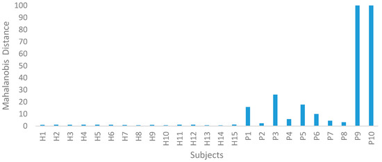
Figure 3. Mahalanobis distance for the healthy group (HG) and ACLR group (PG).

Step II: Validation of MS

In Step II of the MTS, the ACLR data were utilised to confirm the MS dimension scale. Using the averages and standard deviations of the HG data, the PG data were normalised. The MDs of the ACLR group were computed using the covariance coefficient matrix of the HG data. From this study, they were clearly outside of this MS. Therefore, the MS is valid. A wide range of MD values were observed for the PG; on the other hand, the HG was absolutely uniform, as shown in Figure 3. For clinical diagnosis, the main challenge is to obtain a threshold T which differentiates between healthy and ACLR patients. Its distribution is displayed in the graph in Figure 3. As shown in Table 8 the threshold was set at 0.5–3.0 in order to calculate the g-means. After considering sensitivity and specificity, we discovered the best threshold value was 1.5, which provided 100% sensitivity and specificity. The 10 ACLR spatiotemporal data, along with the calculated MDs, are functioned and displayed in Table 9.

Table 8. Sensitivity analysis of the threshold.

Threshold		ACLR (Abnormal)	Healthy (Normal)	Sensitivity (%)	Specificity (%)	G-Means (%)
0.5	Positive	10	0	100	0.00	0.00
	Negative	15	0
1.0	Positive	10	0	100	53.33	73
	Negative	7	8
1.5	Positive	10	0	100	100	100
	Negative	0	15
2.0	Positive	10	0	100	100	100
	Negative	0	15

Table 9. MD for ACLR group (PG) data.

PG	X1	X2	X3	X4	X5	X6	X7	X8	X9	X10	X11	MD
P1	0.52	1.05	0.202	0.96	0.55	1.15	0.46	63.7	28.8	0.38	39.55	15.77
P2	0.55	1.05	0.189	0.84	0.54	1.01	0.34	61.0	25.2	0.48	43.25	2.308
P3	0.51	1.08	0.232	1.08	0.55	1.14	0.47	66.3	29.3	0.39	36.74	26.035
P4	0.58	1.12	0.172	1.03	0.62	1.16	0.46	62.3	28.6	0.38	36.18	5.721
P5	0.57	1.11	0.217	0.98	0.73	1.34	0.42	57.2	24.0	0.36	34.95	17.78
P6	0.60	1.26	0.051	0.68	0.55	1.02	0.20	55.0	16.8	0.59	48.58	9.979
P7	0.56	1.14	0.149	1.08	0.66	1.29	0.43	62.1	24.9	0.38	34.38	4.404
P8	0.59	1.20	0.086	0.75	0.53	1.05	0.27	58.3	20.4	0.51	46.69	3.133
P9	0.54	0.55	0.136	1.26	0.72	0.57	0.46	63.7	44.9	0.29	30.22	1287.16
P10	0.55	1.18	0.102	0.92	0.56	0.48	0.35	61.8	42.5	0.44	40.32	1509.81
Average												288.21

Step III: Identification of useful features.

In Step III of the MTS, OAs and S/N ratios were used to examine the effects of every feature. Since 11 attributes were assembled, an L₁₂ (2¹¹) OA was used. As revealed in Table 10 and Table 11, X1, X2, and X8 did not have a significant effect on the MD. Hence, the number of attributes was decreased from 11 to 8. The PG could be clearly distinguished from the HG group as their MDs deviated significantly in the MS (PG: 2.308–1509.811, HG: 0.560–1.190). In Step III of the MTS, OAs and S/N ratios were used to examine the effects of every feature. Since 11 attributes were assembled, an L₁₂ (2¹¹) OA was used.

Table 10. L₁₂ (2¹¹) OA for the ACLR conditions.

Run	Features											S/N Ratio
	X1	X2	X3	X4	X5	X6	X7	X8	X9	X10	X11
1	1	1	1	1	1	1	1	1	1	1	1	8.49550614
2	1	1	1	1	1	2	2	2	2	2	2	1.31702001
3	1	1	2	2	2	1	1	1	2	2	2	−1.4245509
4	1	2	1	2	2	1	2	2	1	1	2	5.12522506
5	1	2	2	1	2	2	1	2	1	2	1	3.6517743
6	1	2	2	2	1	2	2	1	2	1	1	0.67514098
7	2	1	2	2	1	1	2	2	1	2	1	2.99885419
8	2	1	2	1	2	2	2	1	1	1	2	3.19462065
9	2	1	1	2	2	2	1	2	2	1	1	3.29197259
10	2	2	2	1	1	1	1	2	2	1	2	2.85909121
11	2	2	1	2	1	2	1	1	1	2	2	3.71676119
12	2	2	1	1	2	1	2	1	2	2	1	2.65860164

Table 11. Average S/N ratios and gain for each feature.

	X1	X2	X3	X4	X5	X6	X7	X8	X9	X10	X11
Level-1	2.9733	2.978	4.1	3.696	3.343	3.4521	3.501	2.886	4.5304	3.94	3.628
Level-2	3.1199	3.1144	1.9924	2.397	2.75	2.641	2.662	3.207	1.563	2.153	2.464
Gain	−0.1466	−0.1364	2.1076	1.299	0.593	0.8111	0.839	-0.321	2.9674	1.787	1.164

Step IV: Future diagnosis

The MTS can be applied to achieve two major objectives: diagnosis and forecasting. As shown in Figure 3, the MDs of the 10 ACLR participants are outside of the MS [21]. Therefore, the suggested approach could be used to diagnose ACLR patients. The role of these MDs is to assess the patient, monitor their progress, and to give advice and provide education on the progress of their rehabilitation. The specific exercises provided are extremely important as they are designed to help patients regain a full range of movement and to strengthen the muscles around their knee. Consequently, smaller MDs may be used as the top analytical index to find out if patients are able to fully RTW following ACLR.

5. ACLR Classification

In conventional strategies, such as discrimination and classification strategies (and sometimes in multiple regression), the objective is to classify observations into different groups (populations). In contrast, the main goal of the technique proposed in this research is to supply measurements and to measure the degree of abnormalities on a continuous scale. This can help to determine the correct actions to take predicated by the degree of abnormality [42].

However, in the MTS methods, there are simply no populations [19,24,38,48,49]. It simply requires several observations, called a ‘healthy’ group, to acquire a correlation structure and to define the reference indication for the measurement scale MS. Selection of this healthy group is completely at the discretion of clinicians. In MTS strategies, every irregular condition (ACLR individuals) is considered exclusively, since the occurrence of such conditions differ. The degree of abnormality can be measured in reference to the healthy group [40,43,50,51].To produce the referenced area, MS feature data units from the HG were utilised. The MDs of HG range from 0.560 to 1.180, calculated from the methods introduced in Table 7. The 10 ACLR subjects were used for MS validation [19,24].

The PG data were normalised using the mean and standard deviation of the HG. Their MDs, which were calculated with the covariance coefficient matrix of the HG, range between 2.308 and 1509.811; these are outside of the MS. Therefore, the MS is certainly validated. Hence, Taguchi strategies were used to study the impact of every feature [43,52,53]. The ‘Gain’ of every feature was computed between these two conditions. As shown in DF, X2, and X8 were found to have an insignificant effect on the MD. Hence, the number of features decreased from 11 to 8.

6. ACLR Diagnosis and RTW

6.1. ACLR Diagnosis

Gait variability, defined as the fluctuation in gait features from one step to the next, is an important indicator of impaired mobility in ACLR patients [36,54,55]. In this study, eight important features, including step width, swing time (s), stance time (s), double support time (s), single support time (s), double support time (%GC), gait speed (m/s), and stride speed, were selected by utilising OAs and S/N ratios. These essential features will be discussed in detail.

The human body’s degree of stability can be predicted from step width [56]. In many studies, the step width is often associated with local and orbital stability [54,57]. Stability is defined as the capability of a body to respond to perturbations [58]. During human walking, increasing the step width changes both the anterior-posterior and mediolateral stability along with stability variability [59].

Stance time was identified as a significant variable in clinical gait analysis. According to Kuo and Donelan, modifications in stance time may result in increased mechanical function and, therefore, greater energy consumption during walking [58]. For example, a decline in a single limb’s stance time may result in a heightened contralateral limb swing speed, which will decrease the effect produced by initial contact [2]. Hence, this strategy raises energy expenditure [2]. Therefore, the analysis of stance time is essential as an indicator of subjects’ energy expenditure.

The time from toe-off to the next heel strike, indicating as a passive movement with little metabolic cost, is known as swing time [60]. Current estimates for leg swing costs are equivocal, covering a range of between 10% and 33% of the net cost of walking [60]. Most of the changes were observed during the longer swing period of ACLR patients. As this speed rises, there is a general increase in activity that leads to an increase in muscle strength generation and ground reaction force [31]. Additionally, the increase in speed will decrease stance time, limiting the amount of time that the body needs to explore the various ranges of movement required to accomplish a task [61].

Gait speed has been recognised as a significant factor in normal health condition [62]. Under normal conditions, a comfortable gait speed relates to the speed where the energy cost per unit of distance is minimised [63]. Achieving energy efficiency is dependent on joint mobility and muscle activity [64]. ACLR leads to increased energy use, which is usually accompanied by a compensatory drop in the gait speed. In addition, the motions may cause the centre of gravity to shift, which increases energy expenditure [65].

Stride speed is another important indicator of knee joint health, as well as overall health [56,66]. Slower stride speeds have been associated with poorer results on psychomotor tests, verbal fluency tests, and decreased cardiovascular health [67]. Stride speed has been used as a measure to predict survival rates in an elderly community [68,69]. Stride speed is a good measure of energy, motor control, endurance, muscle function, and health status.

The ACLR knees demonstrated prolonged double support phases and reduced single support phases in comparison to the healthy knees. This reflects the increased time that the ACLR knees tended to remain in flexion prior maximum extension in order to achieve a less sudden weight change. This adaptation mechanism has been also shown by an electromyography experiment, which demonstrated that ACLR patients had prolonged firing of biceps, femoris, and vastus medialis during the stance phase in comparison to the HG [70].

6.2. Return to Work

To date, RTW analysis has concentrated on the knee-demanding workload and the number of weeks walking using crutches. The information is controversial, and there is no general agreement to quantify knee extension and knee function. Previously, the most powerful factor determining RTW after ACLR was the level of knee-demanding work, which is assessed using the work rehabilitation questionnaire (WORQ). Kievit et al. highlight that the time required to completely RTW following ACLR is less than that following a complete knee arthroplasty; with 71% of ACL patients taking more than three months to RTW compared to 50% of total knee arthroplasty patients. However, there no other research describing RTW after knee-related medical procedures was available.

Another factor that has been connected to RTW is the number of weeks the patient requires crutches to walk after the operation [4]. The substantial index, with an odds ratios (OR) of 1.54, suggests that for every week the individual walks using crutches, the danger of a protracted RTW increases by a factor of 1.54 [4]. This suggests that after four months, the OR climbs to 4.57. However, the weakness of this research is that working with the support of crutches actually increases the chance of RTW [4].

Considering the arguments mentioned previously, the MTS ought to be regarded as the most effective program for predicting RTW. This system allows the clinician to identify the principal factors preventing patients from returning to work after the first couple of weeks, and to understand the elements that guarantee RTW. The spatiotemporal information of walking after ACLR has not been analysed previously, so far as we understand. In addition, this method could be implemented to evaluate whether an individual can begin functioning.

Furthermore, specific recommendations for therapy and RTW following knee operations can be provided. The MD may be utilised to determine when patients can fully RTW. It should be observed that the average value of the MD for ACLR individuals, given in Table 9 (typical MD = 288.211), is higher than that of the healthy individuals, given in Table 7 (average MD = 0.933), for the all of the 11 attributes. According to these MD values, the patients could possibly be rated in an ascending sequence. It is obvious that for lower MD values, the deviation from healthy participants is likely be less and the patients will have an excellent likelihood of RTW [31]. From the results, subjects 2, 7, and 8 have an MD close to that of the healthy participants. For individuals with greater MD values, constant rehabilitation should continue until the MD [23].

7. Application

Since one of the goals of restoration of anterior cruciate ligament (ACL) is to return patients to their level of pre-injury activity, it is critical to understand factors that induce. Current guidelines for evaluating an ACLR patient’s results are primarily based on clinicians’ decisions and experience. These guidelines usually consist of qualitative assessment of early intervention plans that emphasizes restoring flexibility, muscular strength, and ligament stability by using closed kinetic chain exercises [71,72,73]. However, a major problem with this kind of qualitative assessment is the clinician’s capacity to provide safe, high-quality care can be reliant on their ability to reason, think, and judge, which can be restricted by absence of experience [74,75]. This is definitely accompanied by several exams to verify the medical diagnosis. For that reason, diagnosing without acquiring assistance from the help of intelligence systems is time consuming.

Therefore, study on medical apps in computerized intelligence systems with MTS is essential. In addition, the implementation of computerized health-related decision support scheme of MTS turns out to be a viable alternative for a quick plus precise patient medical diagnosis. Medical information therefore needs classification approaches with a mixed decision support scheme to guarantee that digital access to health care information will be much simpler for medical officers.

In fact, the system is capable of eliminating any unnecessary items in the information system, as well as offering useful data to the medical officer to assist in making decisions during diagnosis of disease. In addition, MTS is not only capable of performing classification duties, it also has the capacity to recognise the significant multivariate system variables. Furthermore, MTS is not only efficient in performing classification employment, it also provides the ability to determine the key multivariate system parameters. Mahalanobis Space (MS) is developed mainly on the basis of healthy people in the medical diagnosis.

By combining this presented method with the development of sensing technologies, embedded systems, wireless communication technologies, nano-technologies, and miniaturization, smart systems can be developed to monitor human actions on an ongoing basis. Mobile and wearable sensor technology is a rapidly growing sector with a strong potential for health care and scientific study transformation [76,77,78].

Wearable body-sensor network technology is currently moving into routine clinical work, complementing sophisticated motion evaluation with stationary and complicated kinematographic analysis [79,80].These wearable motion sensor systems are suitable for everyday gait assessment, providing a means of delivering individualized gait objectively [81,82,83]. Video-based motion capture systems or instrumented walkway systems are regarded the gold standard for capturing gait parameters, but are expensive and involve dedicated movement labs [78,84].

By implementing MTS and adapting equipment such as wearable sensor-based gait analysis to capture disease status, it can fulfill the requirements of both the doctor, patient and caregiver.

8. Conclusions

In this study, the MTS system was suggested as a way to estimate the health of ACLR patients before they return to work. By building feature data, ACLR diagnosis and classification were achieved using MDs corresponding to different health conditions. The MDs were improved by Taguchi techniques to recognise the attributes that had the greatest impact. ACLR patients are considered ready to RTW when the MDs are small and within the MS. When the MDs are larger, and outside the MS, this suggests that there are problems affecting the individual. In particular, as gait deviation increases, the MD increases. The results demonstrated that the MDs corresponding to the ACLR group deviated from the ones that were healthy. In addition, the size of the MD reflected the degree of abnormality. Hence, MDs can indicate the seriousness of an abnormality. In the future, this MTS method can help physiotherapists to decide comprehensive treatment plans. Further research is essential to optimally target deficits in neuromuscular control, neuromotor status, and psychological readiness in order to best prepare individuals for RTW following ACLR.

References

- Gokeler, A.; Benjaminse, A.; van Eck, C.F.; Webster, K.E.; Schot, L.; Otten, E. Return of normal gait as an outcome measurement in acl reconstructed patients. A systematic review. Int. J. Sports Phys. Ther. 2013, 8, 441–451. [Google Scholar] [PubMed]
- Leporace, G.; Metsavaht, L.; Zeitoune, G.; Marinho, T.; Oliveira, T.; Pereira, G.R.; De Oliveira, L.P.; Batista, L.A. Use of spatiotemporal gait parameters to determine return to sports after ACL reconstruction. Acta Ortop. Bras. 2016, 24, 73–76. [Google Scholar] [CrossRef]
- Johnson, R.J.; Beynnon, B.D. What do we really know about rehabilitation after ACL reconstruction?: commentary on an article by L.M. Kruse, MD, et al.: “rehabilitation after anterior cruciate ligament reconstruction. a systematic review.”. J. Bone Jt. Surg Am. 2012, 94, e148(1-2). [Google Scholar] [CrossRef] [PubMed][Green Version]
- Groot, J.A.M.; Jonkers, F.J.; Kievit, A.J.; Kuijer, P.P.F.M.; Hoozemans, M.J.M. Beneficial and limiting factors for return to work following anterior cruciate ligament reconstruction: a retrospective cohort study. Arch. Orthop. Trauma Surg. 2017, 137, 155–166. [Google Scholar] [CrossRef]
- Meuffels, D.E.; Poldervaart, M.T.; Diercks, R.L.; Fievez, A.W.F.M.; Patt, T.W.; Van Der Hart, C.P.; Hammacher, E.R.; Van Der Meer, F.; Goedhart, E.A.; Lenssen, A.F.; et al. Guideline on anterior cruciate ligament injury. Acta Orthop. 2012, 83, 379–386. [Google Scholar] [CrossRef] [PubMed]
- Herrington, L.; Myer, G.; Horsley, I. Task based rehabilitation protocol for elite athletes following Anterior Cruciate ligament reconstruction: A clinical commentary. Phys. Ther. Sport 2013, 14, 188–198. [Google Scholar] [CrossRef] [PubMed]
- Lyman, S.; Koulouvaris, P.; Sherman, S.; Do, H.; Mandl, L.A.; Marx, R.G. Epidemiology of anterior cruciate ligament reconstruction. Trends, readmissions, and subsequent knee surgery. J. Bone Jt. Surg. - Ser. A 2009, 91, 2321–2328. [Google Scholar] [CrossRef]
- Everhart, J.S.; Best, T.M.; Flanigan, D.C. Psychological predictors of anterior cruciate ligament reconstruction outcomes: a systematic review. Knee Surgery Sport. Traumatol. Arthrosc. 2015, 23, 752–762. [Google Scholar] [CrossRef]
- Wilk, K.E.; Arrigo, C.; Andrews, J.R.; Clancy, W.G. Rehabilitation after anterior cruciate ligament reconstruction in the female athlete. J. Athl. Train. 1999, 34, 177–193. [Google Scholar]
- Di Stasi, S.; Hartigan, E.H.; Snyder-Mackler, L. Sex-specific gait adaptations prior to and up to 6 months after anterior cruciate ligament reconstruction. J. Orthop. Sports Phys. Ther. 2015, 45, 207–214. [Google Scholar] [CrossRef]
- Magnussen, R.A.; Pedroza, A.D.; Donaldson, C.T.; Flanigan, D.C.; Kaeding, C.C. Time from ACL injury to reconstruction and the prevalence of additional intra-articular pathology: is patient age an important factor? Knee Surg Sport. Traumatol Arthrosc 2013. [Google Scholar] [CrossRef] [PubMed]
- Pamukoff, D.N.; Pietrosimone, B.G.; Ryan, E.D.; Lee, D.R.; Blackburn, J.T. Quadriceps Function and Hamstrings Co-Activation After Anterior Cruciate Ligament Reconstruction. J. Athl. Train. 2017, 52, 422–428. [Google Scholar] [CrossRef] [PubMed]
- Pamukoff, D.N.; Pietrosimone, B.; Lewek, M.D.; Ryan, E.D.; Weinhold, P.S.; Lee, D.R.; Blackburn, J.T. Whole body and local muscle vibration immediately improves quadriceps function in individuals with anterior cruciate ligament reconstruction. Arch. Phys. Med. Rehabil. 2016. [Google Scholar] [CrossRef] [PubMed]
- Toutoungi, D.E.; Lu, T.W.; Leardini, A.; Catani, F.; O’Connor, J.J. Cruciate ligament forces in the human knee during rehabilitation exercises. Clin. Biomech. 2000, 15, 176–187. [Google Scholar] [CrossRef]
- Kuenze, C.; Hertel, J.; Weltman, A.; Diduch, D.R.; Saliba, S.; Hart, J.M. Jogging biomechanics after exercise in individuals with ACL-Reconstructed knees. Med. Sci. Sports Exerc. 2014, 46, 1067–1076. [Google Scholar] [CrossRef] [PubMed]
- Ryan, Z.; Mathew, F. Lynn Snyder-Mackler The relationship between EMG activity and psychological outlook following ACL reconstruction. J. Orthop. Res. 2016, 34. [Google Scholar]
- Atkinson, H.D.E.; Laver, J.M.; Sharp, E. (vi) Physiotherapy and rehabilitation following soft-tissue surgery of the knee. Orthop. Trauma 2010, 24, 129–138. [Google Scholar] [CrossRef]
- Taguchi, R.; Jugulum, G. The Mahalanobis–Taguchi Strategy—A Pattern Technology System; John Wiley and Sons Inc.: Hoboken, NJ, USA, 2002. [Google Scholar]
- Wang, P.C.; Su, C.T.; Chen, K.H.; Chen, N.H. The application of rough set and Mahalanobis distance to enhance the quality of OSA diagnosis. Expert Syst. Appl. 2011, 38, 7828–7836. [Google Scholar] [CrossRef]
- Aly, S. Learning invariant local image descriptor using convolutional Mahalanobis self-organising map. Neurocomputing 2014, 142, 239–247. [Google Scholar] [CrossRef]
- Long, B.; Xian, W.; Li, M.; Wang, H. Improved diagnostics for the incipient faults in analog circuits using LSSVM based on PSO algorithm with Mahalanobis distance. Neurocomputing 2014, 133, 237–248. [Google Scholar] [CrossRef]
- Hsiao, Y.H.; Su, C.T.; Fu, P.C.; Chen, M.C. MTSbag: A Method to Solve Class Imbalance Problems. In Proceedings of the 2018 7th International Congress on Advanced Applied Informatics (IIAI-AAI), Yonago, Japan, 8–13 July 2018; pp. 524–529. [Google Scholar] [CrossRef]
- Haldar, N.A.H.; Khan, F.A.; Ali, A.; Abbas, H. Arrhythmia classification using Mahalanobis distance based improved Fuzzy C-Means clustering for mobile health monitoring systems. Neurocomputing 2017, 220, 221–235. [Google Scholar] [CrossRef]
- Su, C.T.; Hsiao, Y.H. An evaluation of the robustness of MTS for imbalanced data. IEEE Trans. Biomed. Eng. 2007, 19, 1321–1332. [Google Scholar] [CrossRef]
- Maitland, M.E.; Bell, G.D.; Mohtadi, N.G.H.; Herzog, W. Quantitative analysis of anterior cruciate ligament instability. Clin. Biomech. 1995, 10, 93–97. [Google Scholar] [CrossRef]
- White, K.; Logerstedt, D.; Snyder-Mackler, L. Gait Asymmetries Persist 1 Year After Anterior Cruciate Ligament Reconstruction. Orthop. J. Sport. Med. 2013, 1, 1–6. [Google Scholar] [CrossRef] [PubMed]
- Sigward, S.M.; Lin, P.; Pratt, K. Knee loading asymmetries during gait and running in early rehabilitation following anterior cruciate ligament reconstruction: A longitudinal study. Clin. Biomech. 2016, 32, 249–254. [Google Scholar] [CrossRef] [PubMed]
- Lohmander, L.S.; Englund, P.M.; Dahl, L.L.; Roos, E.M. The long-term consequence of anterior cruciate ligament and meniscus injuries: osteoarthritis. Am. J. Sport. Med 2007, 35, 1756–1769. [Google Scholar] [CrossRef]
- Wellsandt, E.; Arundale, A.; Manal, K.; Buchanan, T.S.; Snyder-Mackler, L. Lower hop scores related to gait asymmetries after ACL injury: Identifying associations related to the development of early onset knee OA. Osteoarthr. Cartil. 2015, 23, A279. [Google Scholar] [CrossRef]
- Hart, H.F.; Collins, N.J.; Ackland, D.C.; Cowan, S.M.; Crossley, K.M. Gait Characteristics of People With Lateral Knee OA After ACL Reconstruction. Med. Sci. Sports Exerc. 2015, 2406–2415. [Google Scholar] [CrossRef]
- Paterno, M.V.; Schmitt, L.C.; Ford, K.R.; Rauh, M.J.; Hewett, T.E. Altered postural sway persists after anterior cruciate ligament reconstruction and return to sport. Gait Posture 2013, 38, 136–140. [Google Scholar] [CrossRef]
- Heijne, A. Rehabilitation After Anterior Cruciate Ligament Reconstruction Using Patellar Tendon or Hamstring Grafts: Open and Closed Kinetic Chain Exercises. Ph.D. Thesis, Karolinska Institutet, Solna, Sweden, 2007. [Google Scholar]
- Fithian, D.C.; Powers, C.M.; Khan, N. Rehabilitation of the Knee After Medial Patellofemoral Ligament Reconstruction. Clin. Sports Med. 2010, 29, 283–290. [Google Scholar] [CrossRef]
- Barber-Westin, S.D.; Noyes, F.R. Objective criteria for return to athletics after anterior cruciate ligament reconstruction and subsequent reinjury rates: a systematic review. Phys. Sportsmed. 2011, 39, 100–110. [Google Scholar] [CrossRef] [PubMed]
- Webster, K.E.; Wittwer, J.E.; O’Brien, J.; Feller, J.A. Gait Patterns After Anterior Cruciate Ligament Reconstruction Are Related to Graft Type. Am. J. Sports Med. 2005, 33, 247–254. [Google Scholar] [CrossRef] [PubMed]
- Culvenor, A.G.; Perraton, L.; Guermazi, A.; Bryant, A.L.; Whitehead, T.S.; Morris, H.G.; Crossley, K.M. Knee kinematics and kinetics are associated with early patellofemoral osteoarthritis following anterior cruciate ligament reconstruction. Osteoarthr. Cartil. 2016, 24, 1548–1553. [Google Scholar] [CrossRef] [PubMed]
- Butler, R.J.; Minick, K.I.; Ferber, R.; Underwood, F. Gait mechanics after ACL reconstruction: Implications for the early onset of knee osteoarthritis. Br. J. Sports Med. 2009, 43, 366–370. [Google Scholar] [CrossRef] [PubMed]
- Hsiao, Y.H.; Su, C.T. Multiclass MTS for saxophone timbre quality inspection using waveform-shape-based features. IEEE Trans. Syst. Man, Cybern. Part B Cybern. 2009, 39, 690–704. [Google Scholar] [CrossRef] [PubMed]
- Song, J.L.; Hu, W.; Zhang, R. Automated detection of epileptic EEGs using a novel fusion feature and extreme learning machine. Neurocomputing 2015, 175, 383–391. [Google Scholar] [CrossRef]
- Taguchi, G.; Jugulum, R. The Mahalanobis–Taguchi Strategy; John Wiley Sons Inc.: Hoboken, NJ, USA, 2002. [Google Scholar] [CrossRef]
- Fearn, T. Taguchi methods. NIR News 2001, 12, 2013. [Google Scholar] [CrossRef]
- Ali, A.; Haldar, N.A.H.; Khan, F.A.; Ullah, S. ECG arrhythmia classification using mahalanobis-taguchi system in a body area network environment. In Proceedings of the 2015 IEEE Global Communications Conference (GLOBECOM), San Diego, CA, USA, 6–10 December 2015. [Google Scholar] [CrossRef]
- Su, C. Mahalanobis – Taguchi System and Its Medical Applications. Neuropsychiatry 2017, 7, 316–320. [Google Scholar]
- Sadeghi, H.; Allard, P.; Prince, F.F.; Labelle, H. Symmetry and limb dominance in able-bodied gait: a review. Gait Posture 2000, 12, 34–45. [Google Scholar] [CrossRef]
- Morgan, K.D.; Zheng, Y.; Bush, H.; Noehren, B. Nyquist and Bode stability criteria to assess changes in dynamic knee stability in healthy and anterior cruciate ligament reconstructed individuals during walking. J. Biomech. 2016. [Google Scholar] [CrossRef]
- Chmielewski, T.L.; Hurd, W.J.; Rudolph, K.S.; Axe, M.J.; Snyder-mackler, L. Kinematics and Reduces Muscle. Phys. Ther. 2005, 85, 740–754. [Google Scholar]
- Goerger, B.M.; Marshall, S.W.; Beutler, A.I.; Blackburn, J.T.; Wilckens, J.H.; Padua, D.A. Anterior cruciate ligament injury alters preinjury lower extremity biomechanics in the injured and uninjured leg: The JUMP-ACL study. Br. J. Sports Med. 2015, 49, 188–195. [Google Scholar] [CrossRef]
- Iquebal, A.S.; Pal, A.; Ceglarek, D.; Tiwari, M.K. Enhancement of Mahalanobis-Taguchi System via Rough Sets based Feature Selection. Expert Syst. Appl. 2014, 41, 8003–8015. [Google Scholar] [CrossRef]
- Lee, Y.C.; Teng, H.L. Predicting the financial crisis by Mahalanobis-Taguchi system - Examples of Taiwan’s electronic sector. Expert Syst. Appl. 2009, 36, 7469–7478. [Google Scholar] [CrossRef]
- Pal, A.; Maiti, J. Development of a hybrid methodology for dimensionality reduction in Mahalanobis–Taguchi system using Mahalanobis distance and binary particle swarm optimization. Expert Syst. Appl. 2010, 37, 1286–1293. [Google Scholar] [CrossRef]
- Jin, X.; Chow, T.W.S. Anomaly detection of cooling fan and fault classification of induction motor using Mahalanobis–Taguchi system. Expert Syst. Appl. 2013, 40, 5787–5795. [Google Scholar] [CrossRef]
- Buenviaje, B.; Bischoff, J.; Roncace, R.; Willy, C. Mahalanobis Taguchi System to Identify Pre- indicators of Delirium in the ICU. Biomed. Heal. Inform. IEEE J. 2015, 20, 1205–1212. [Google Scholar] [CrossRef]
- Reséndiz, E.; Rull-Flores, C.A. Mahalanobis-Taguchi system applied to variable selection in automotive pedals components using Gompertz binary particle swarm optimization. Expert Syst. Appl. 2013, 40, 2361–2365. [Google Scholar] [CrossRef]
- Williams, A.A.; Titchenal, M.R.; Andriacchi, T.P.; Chu, C.R. MRI UTE-T2* profile characteristics correlate to walking mechanics and patient reported outcomes 2 years after ACL reconstruction. Osteoarthr. Cartil. 2018, 26, 569–579. [Google Scholar] [CrossRef]
- Bhatla, J.L.; Kroker, A.; Manske, S.L.; Emery, C.A.; Boyd, S.K. Differences in subchondral bone plate and cartilage thickness between women with anterior cruciate ligament reconstructions and uninjured controls. Osteoarthr. Cartil. 2018, 26, 929–939. [Google Scholar] [CrossRef]
- Boggess, G.; Morgan, K.; Johnson, D.; Ireland, M.L.; Reinbolt, J.A.; Noehren, B. Neuromuscular compensatory strategies at the trunk and lower limb are not resolved following an ACL reconstruction. Gait Posture 2018, 60, 81–87. [Google Scholar] [CrossRef]
- Mitchell, M.J.; King, M.R. Voluntarily Changing Step Length or Step Width Affects Dynamic Stability of Human Walking. New J. Phys. 2014, 35, 1–23. [Google Scholar] [CrossRef]
- Kuo, A.D.; Donelan, J.M. Dynamic Principles of Gait and Their Clinical Implications. Phys. Ther. 2010, 90, 157–174. [Google Scholar] [CrossRef]
- Young, P.M.M.; Wilken, J.M.; Dingwell, J.B. Dynamic Margins of Stability During Human Walking in Destabilizing Environments. J. Biomech. 2012, 45, 1053–1059. [Google Scholar] [CrossRef]
- Umberger, B.R.; Umberger, B.R. Stance and swing phase costs in human walking Stance and swing phase costs in human walking. J. R. Soc. Interface 2010, 7, 1329–1340. [Google Scholar] [CrossRef]
- Gribbin, T.C.; Slater, L.V.; Herb, C.C.; Hart, J.M.; Chapman, R.M.; Hertel, J.; Kuenze, C.M. Differences in hip-knee joint coupling during gait after anterior cruciate ligament reconstruction. Clin. Biomech. 2016, 32, 64–71. [Google Scholar] [CrossRef]
- Lin, P.E.; Sigward, S.M. Contributors to knee loading deficits during gait in individuals following anterior cruciate ligament reconstruction. Gait Posture 2018. Under review. [Google Scholar] [CrossRef]
- Kurz, M.J.; Stergiou, N.; Buzzi, U.H.; Georgoulis, A.D. The effect of anterior cruciate ligament recontruction on lower extremity relative phase dynamics during walking and running. Knee Surg. Sport. Traumatol. Arthrosc. 2005, 13, 107–115. [Google Scholar] [CrossRef]
- Franceschini, M.; Rampello, A.; Agosti, M.; Massucci, M.; Bovolenta, F.; Sale, P. Walking Performance: Correlation between Energy Cost of Walking and Walking Participation. New Statistical Approach Concerning Outcome Measurement. PLoS One 2013, 8. [Google Scholar] [CrossRef]
- Esquenazi, A. Gait analysis in lower-limb amputation and prosthetic rehabilitation. Phys. Med. Rehabil. Clin. N. Am. 2014, 25, 153–167. [Google Scholar] [CrossRef]
- Armitano, C.N.; Morrison, S.; Russell, D.M. Upper body accelerations during walking are altered in adults with ACL reconstruction. Gait Posture 2017, 58, 401–408. [Google Scholar] [CrossRef] [PubMed]
- Van Egmond, M.A.; van der Schaaf, M.; Vredeveld, T.; Vollenbroek-Hutten, M.M.R.; van Berge Henegouwen, M.I.; Klinkenbijl, J.H.G.; Engelbert, R.H.H. Effectiveness of physiotherapy with telerehabilitation in surgical patients: a systematic review and meta-analysis. Physiotherapy 2018. [Google Scholar] [CrossRef] [PubMed]
- Studenski, S.; Perera, S.; Patel, K. Gait Speed and Survival in Older Adults. Jama 2011, 305, 50–58. [Google Scholar] [CrossRef] [PubMed]
- Gao, B.; Zheng, N. (Nigel) Alterations in three-dimensional joint kinematics of anterior cruciate ligament-deficient and -reconstructed knees during walking. Clin. Biomech. 2010, 25, 222–229. [Google Scholar] [CrossRef] [PubMed]
- Knoll, Z.; Kiss, R.M.; Kocsis, L. Gait adaptation in ACL deficient patients before and after anterior cruciate ligament reconstruction surgery. J. Electromyogr. Kinesiol. 2004, 14, 287–294. [Google Scholar] [CrossRef] [PubMed]
- Morrissey, M.C.; Hudson, Z.L.; Drechsler, W.I.; Coutts, F.J.; Knight, P.R.; King, J.B. Effects of open versus closed kinetic chain training on knee laxity in the early period after anterior cruciate ligament reconstruction. Knee Surgery, Sport. Traumatol. Arthrosc. 2000, 8, 343–348. [Google Scholar] [CrossRef] [PubMed]
- Isberg, J.; Faxén, E.; Brandsson, S.; Eriksson, B.I.; Kärrholm, J.; Karlsson, J. Early active extension after anterior cruciate ligament reconstruction does not result in increased laxity of the knee. Knee Surgery, Sport. Traumatol. Arthrosc. 2006, 14, 1108–1115. [Google Scholar] [CrossRef] [PubMed]
- Mikkelsen, C.; Werner, S.; Eriksson, E. Closed kinetic chain alone compared to combined open and closed kinetic chain exercises for quadriceps strengthening after anterior cruciate ligament reconstruction with respect to return to sports: A prospective matched follow-up study. Knee Surgery Sport. Traumatol. Arthrosc. 2000, 8, 337–342. [Google Scholar] [CrossRef]
- Moissenet, F.; Armand, S. Qualitative and quantitative methods of assessing gait disorders. In Orthopedic Management Children with Cerebral Palsy A Comprehensive Approach; Nova Biomedical Books: Hauppauge, NY, USA, 2015; pp. 215–240. [Google Scholar]
- Cavanaugh, J.T.; Powers, M. ACL Rehabilitation Progression: Where Are We Now? Curr. Rev. Musculoskelet. Med. 2017, 10, 289–296. [Google Scholar] [CrossRef]
- Galna, B.; Lord, S.; Burn, D.J.; Rochester, L. Progression of gait dysfunction in incident Parkinson’s disease: Impact of medication and phenotype. Mov. Disord. 2015, 30, 359–367. [Google Scholar] [CrossRef]
- Pasluosta, C.F.; Gassner, H.; Winkler, J.; Klucken, J.; Eskofier, B.M. An emerging era in the management of Parkinson’s disease: Wearable technologies and the internet of things. IEEE J. Biomed. Heal. Informatics 2015, 19, 1873–1881. [Google Scholar] [CrossRef]
- Schlachetzki, J.C.M.; Barth, J.; Marxreiter, F.; Gossler, J.; Kohl, Z.; Reinfelder, S.; Gassner, H.; Aminian, K.; Klucken, J.; Eskofier, M. Wearable sensors objectively measure gait parameters in Parkinson’s disease. PLoS ONE 2017, 12, e0183989. [Google Scholar] [CrossRef]
- Horak, F.B.; Mancini, M. Objective biomarkers of balance and gait for Parkinson’s disease using body-worn sensors. Mov. Disord. 2013, 28, 1544–1551. [Google Scholar] [CrossRef]
- Maetzler, W.; Klucken, J.; Horne, M. A clinical view on the development of technology-based tools in managing Parkinson’s disease. Mov. Disord. 2016, 31, 1263–1271. [Google Scholar] [CrossRef]
- Hobert, M.A.; Maetzler, W.; Aminian, K.; Chiari, L. Technical and clinical view on ambulatory assessment in Parkinson’s disease. Acta Neurol. Scand. 2014, 130, 139–147. [Google Scholar] [CrossRef]
- Maetzler, W.; Domingos, J.; Srulijes, K.; Ferreira, J.J.; Bloem, B.R. Quantitative wearable sensors for objective assessment of Parkinson’s disease. Mov. Disord. 2013, 28, 1628–1637. [Google Scholar] [CrossRef]
- Dewey, D.C.; Miocinovic, S.; Bernstein, I.; Khemani, P.; Querry, R.; Chitnis, S.; Dewey, R.B. Automated gait and balance parameters diagnose and correlate with severity in Parkinson disease. J. Neurol. Sci. 2014, 345, 131–138. [Google Scholar] [CrossRef]
- Verghese, J.; Holtzer, R.; Lipton, R.B.; Wang, C. Quantitative gait markers and incident fall risk in older adults. J. Gerontol.- Ser. A Biol. Sci. Med. Sci. 2009, 64, 896–901. [Google Scholar] [CrossRef]
© 2019 by the authors. Licensee MDPI, Basel, Switzerland. This article is an open access article distributed under the terms and conditions of the Creative Commons Attribution (CC BY) license (http://creativecommons.org/licenses/by/4.0/).