Probabilistic Energy Flow Calculation through the Nataf Transformation and Point Estimation

Featured Application

The work presented in this paper provides methods for probabilistic energy flow calculations and will serve as a reference for the operation and maintenance of integrated energy systems.

Abstract

With the increasing capacity of renewable energy sources, uncertainties regarding renewable energy and other dynamic loads in integrated energy systems (IESs) are increasing. Thus, it is necessary to study the probabilistic energy flow (PEF) of IESs. However, existing PEF calculation methods such as the point estimate method (PEM) are computationally inefficient when there are many random variables and estimated points; moreover, relatively large errors can occur when the estimated points are outside their limits. Hence, this paper presents a calculation method that addresses these problems. Because there are correlations among the variables, the Nataf transformation is employed to control the correlation quickly and effectively. A model for an IES that is interconnected with natural gas and electricity systems and accounts for the uncertainties of wind plants, photovoltaic power plants, and dynamic gas loads is presented. Correlations between wind plants and photovoltaic power plants are handled using the Nataf transformation. Finally, a modified PEM is developed to solve the PEF. For situations in which the estimated points exceed their boundaries, the power transformation and equal constraint transformation methods are used. The results of time-domain simulations demonstrate the effectiveness of the proposed approach.

1. Introduction

The increasing demand for energy has resulted in increased concerns regarding energy sources, and the exploration of new energy supply modes has attracted considerable interest. The concept of integrated energy systems (IESs) challenges that of traditional energy systems. IESs, which can fully utilize energy in various forms and optimize resource allocation, have rapidly developed in recent years [1]. Compared with traditional energy systems, these systems have significant advantages [2,3]. For example, all types of energy are closely coupled, which makes them complementary and mutually beneficial, and they can realize cascade utilization and collaborative optimization of energy. Presently, research on IESs is mostly focused on three aspects: energy flow analysis and calculation [4], multi-energy system optimization scheduling [2,3], and multi-energy system planning and multi-market games [5,6].

The ability to integrate various types of energy structures is a compelling advantage of IESs [7,8]. However, owing to the significant amount of renewable energy sources (RESs) involved, crucial challenges in terms of energy uncertainties arise. The uncertainties come from the intermittency of RESs; additionally, the volatility of the loads in different energy structures aggravate the energy uncertainties in IESs [9], which creates significant challenges for the operation and maintenance of IESs. We can determine the probabilistic distribution of each node state in the IESs by calculating the probabilistic energy flow, which provides guidance to address possible risks. Therefore, the probabilistic energy flow (PEF) in IESs must be studied.

The basis of PEF is the calculation of steady-state energy flow (SSEF), which has been studied extensively. Because of the similarity between the SSEF model of the power system and the gas network, Newton’s method can be used to solve the SSEF of the gas network. When the initial point of Newton’s method is near the equilibrium point, the method has good and fast convergence. Moreover, the IES mostly works near the equilibrium point. Therefore, Newton’s method is a commonly used method for solving the energy flow problem. Moreover, the solutions obtained using this method for multiple energy systems can be divided into two forms according to the Jacobian matrices used in the solution, i.e., separate Newton iterations for each system [10] or a unified Newton iteration for all systems [11]. In [10], each energy system (e.g., power system or natural gas system) is represented by its own Jacobian matrix and independent iterations are performed using Newton’s method. The unbalanced quantity is iterated using the energy coupling unit until the whole energy system achieves convergence. This method is relatively simple, but the computation speed is somewhat slow. In [11], the power and natural gas networks are represented by a single Jacobian matrix for the unified Newton iterations. Then, the integrated energy flow of the entire network can be obtained. This method is more complicated in cases where there is a compressor in the gas grid, but the iterations are faster.

Presently, research on the impact of uncertainties in IESs is limited. However, the calculations performed for these systems are similar to the probabilistic power flow (PPF) calculations in traditional power systems. They include the Monte Carlo method [12], analytical method [13], stochastic spectral analysis method [14], and approximation method [15].

Generally, a Monte Carlo simulation (MCS) requires several samples to obtain good precision according to the law of large numbers; this simulation requires considerable time to compute. However, it is possible to achieve the most accurate results with an MCS; therefore, it is used as reference to measure the precision of other methods. The studies on MCSs mainly focus on improving sampling efficiency to reduce the number of sampling representatives, for instance stratified sampling [16,17] and importance sampling [18]. Others focus on improving the calculation efficiency using methods such as parallel computing [19]. The sampling sequence can also be changed to reduce the number of samples, such as in the quasi-Monte Carlo method [20]. This method obtains random numbers using the Sobol sequence, which generates more uniformity than random numbers generated by the pseudo random number technique.

The analytical method is used to solve the PPF problem with a linearized alternating current model and convolution. The number of calculations in this method increases exponentially when the system is relatively large and several components need to be considered. Therefore, this method is not as widely used as the other three methods.

Stochastic spectral analysis includes the Karhunen–Loeve expansion method (KLEM) [21], polynomial chaos expansion [22], and surrogate modelling [23]. KLEM expands the system response into a deterministic part and a stochastic part. The stochastic part consists of a series of unrelated random variables and deterministic coefficients (eigenvalues and eigenfunctions). The disadvantage of KLEM is that it is not applicable to the covariance function of unknown stochastic processes. Polynomial chaos expansion expands the structural probability using the orthogonal polynomial of the basic variable and uses the chaotic polynomial as the basis of the expansion. Therefore, it can be applied to both Gaussian and non-Gaussian outputs. However, when the number of uncertain parameters increases, the number of polynomial coefficients also increase, which greatly increases the cost of computation. Hence, stochastic spectral analysis method is a new method developed recently and remains an on-going research.

Currently, the approximation method is an important approach to solving the PPF problem. This method mainly includes the first-order second-moment method (FOSMM) [24] and point estimate method (PEM) [25]. The FOSMM is fast and precise. Because it adopts the Taylor series expansion method, only the linear term is considered and the higher-order term is ignored; therefore, when the system is highly nonlinear or the random variables are very asymmetrical, a large error will be caused. PEM is now widely used for solving the PPF problem; through Gaussian interpolation, the estimated points can be easily obtained, resulting in fewer power flow calculations. PEM is very fast. However, the original PEM cannot deal with correlated variables [26] and the estimated points might exceed the estimator boundary constraints, which results in a less accurate result [27]. Therefore, PEM is restricted to specific applications.

However, studies examining cases wherein a great number of probability variables with different marginal distributions co-exist in IESs are scarce. In practice, the probability variables, such as those of RESs, are highly correlated with each other; for example, wind speeds and solar radiation at different sites within the same geographical area are typically dependent owing to similar weather conditions. Thus, large errors will occur if we ignore the correlations among different probability variables. The commonly used approaches to deal with the correlation of random variables are transformation methods such as the third-order polynomial normal transformation (TPNT) [28], rotational transformation and orthogonal transformation (RTOT) [29], Rosenblatt transformation [30], unscented transformation [26], and copula function method (CFM) [20].

TPNT transfers variables into the third-order polynomial normal space, which causes mapping errors and low accuracy in some cases. RTOT transfers the correlation variables from the linear correlation coefficient matrix into the generated samples. Unlike the unscented transformation, which does not require a linear transformation and is suitable for any arbitrary nonlinear function, RTOT is essentially a linear transformation method. CFM uses marginal distribution functions to obtain joint distribution functions; this is a convenient method for adding relevance among variables with good precision, so it is now widely adopted. The Nataf transformation [31], which is a type of Gaussian copula, is one of the most important CFMs and famous for its high precision and speed; it can link any distribution space to the normal distribution space, and this is extremely beneficial for the PEM. The estimated points and weights can be easily obtained through the Gauss–Hermite integration. Moreover, because the calculation of PEF is extremely time consuming, the PEM can considerably reduce the computation time. Therefore, the combination of the Nataf transformation with PEM is an excellent choice for PEF calculations. However, the probability variables can be bounded by constraints. For instance, wind farms have cut-in and cut-out wind speed constraints, and when the estimated points are outside the range of these constraints, they lose their physical significance and cause errors. In particular, when dealing with 2-point and 3-point estimation situations, because of the small number of estimated points, the errors can become considerable. Hence, it is necessary to limit the estimated points to remain within the boundaries of the constraints.

The goal of this study is to solve the PEF in an IES. We comprehensively consider the uncertainty regarding wind energy, solar energy in power systems, and gas loads in natural gas systems to establish a model for calculating the PEF. Considering the correlation between different wind-driven generators and solar energy generators in reality, we propose using the Nataf transformation to solve the correlation problem accurately and efficiently. As is well known, solving the PEF in an IES is more time consuming than solving the PPF in a power system. The Monte Carlo method is an inefficient solution to the PEF; hence, the method developed in our study improves the solution efficiency using the multipoint estimation method (MPEM). This paper proposes an extension to the existing MPEM that reduces the computational complexity and cost. For cases where the estimated points are outside of the range, the approach proposed in this paper uses the power transformation method and equality constraint transformation to improve 2-point and 3-point estimations and reduce the calculation error.

The remainder of this paper is organized as follows: A PEF model for IESs is described in Section 2. A PEM based on the Nataf transformation is detailed in Section 3, and 2-point estimation methods considering boundary constraints are discussed in Section 4. Section 5 presents a case discussing PEF calculations, and Section 6 discusses the ideas proposed in this paper and directions of research worth studying in future. The concluding remarks are given in Section 7. Notations and a list of abbreviations are provided in the Appendix A.

2. PEF Model for IESs

2.1. SSEF Calculation in an IES

The SSEF calculation is the basic step in PEF calculations; similar to the power flow model of power systems, the SSEF model can be expressed using the following equation:

$$\begin{array}{c}p=P_i^s+P_i^g-P_i^l-P_c-{\displaystyle \sum _{j=1}^n{P}_{ij}}=0\\ j\ne i,\forall i=1,\cdot \cdot \cdot ,n\\ q=Q_i^s+Q_i^g-Q_i^l-P_c-{\displaystyle \sum _{j=1}^n{P}_{ij}}=0\\ j\ne i,\forall i=1,\cdot \cdot \cdot ,n\\ f_{NG}=Q_i-{\displaystyle \sum _{m\in i}{f}_{im}}+{\displaystyle \sum _{m\in i}{f}_{in}}+{\displaystyle \sum _j{G}_{ij}{F}_j}=0\\ j\ne i,\forall i=1,\cdot \cdot \cdot ,m\end{array}$$

(1)

Here, $P_i^s$ and $Q_i^s$ are respectively the active and reactive power that the source injects into node $i$, $P_i^l$ and $Q_i^l$ are respectively the active and reactive power demanded by the $ith$ node load, $P_i^c$ and $Q_i^c$ are respectively the active and reactive power consumed by the compressor, and $P_i^g$ and $Q_i^g$ are respectively the active and reactive power that the gas generator injects into node $i$. In addition, $n$ represents the number of nodes directly connected to the $ith$ node, $Q_i$ is the injection of natural gas at the $ith$ node, and $f_{im}$ and $f_{in}$ represent the injections at the downstream and upstream nodes, respectively. The gas consumption of the compressor is denoted by $F_j$: when the compressor takes air from node $i$, the correlation coefficient $G_{ij}$ is 1; otherwise, $G_{ij}$ is 0. If the energy required by the compressor comes from the power system, then $G_{ij}$ is also 0. Finally, $p$, $q$ and $f_{NG}$ represent the active, reactive, and gas flow unbalances in a node.

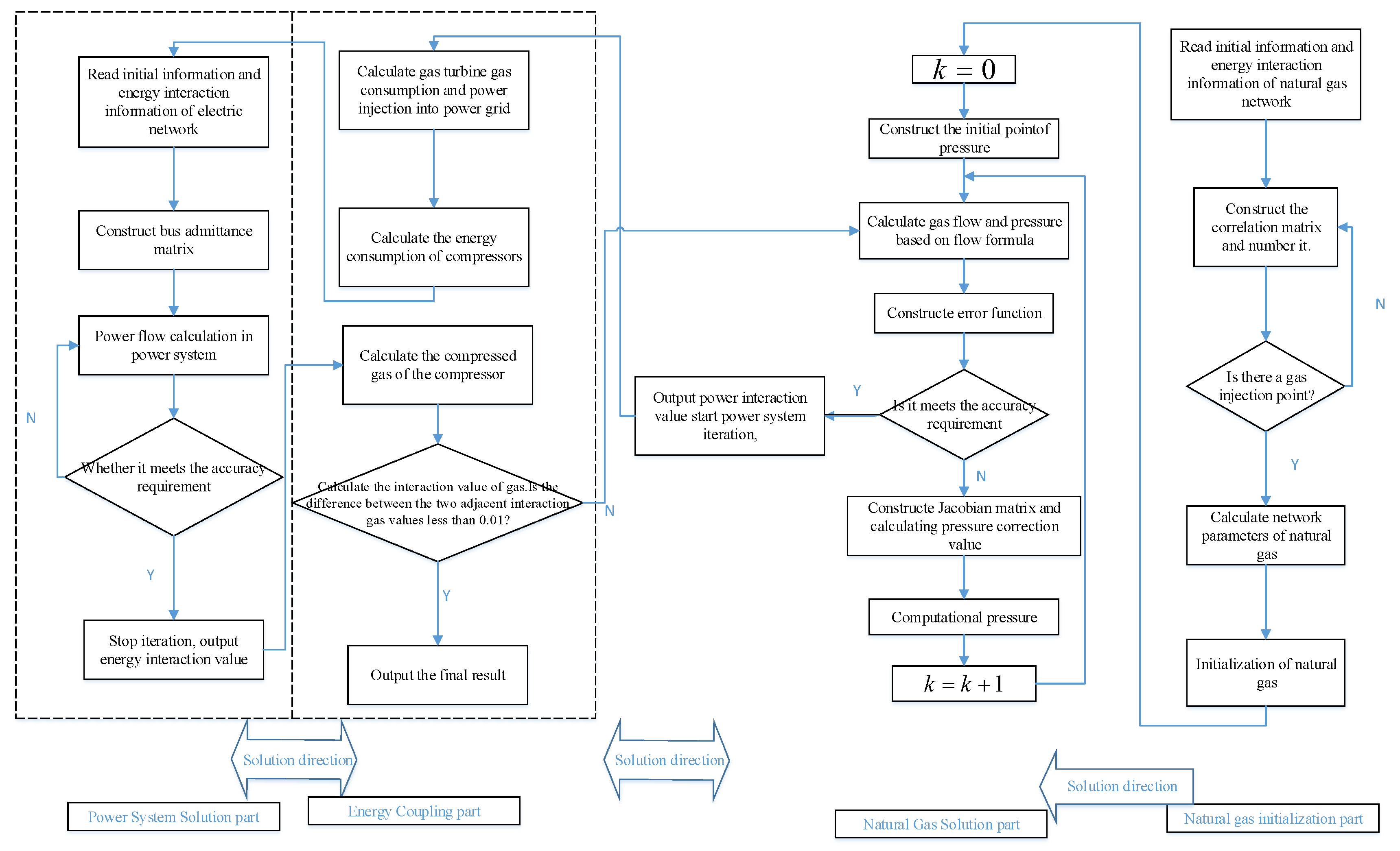
The specific calculation of the SSEF and parameters for a natural gas network are discussed elsewhere [10]. This study uses separate Newton iterations to solve the SSEF problem. That is, the SSEFs of the power and natural gas systems are each iterated independently using Newton’s method until convergence is achieved. Then, the unbalanced quantity between these energy systems is iterated through the energy coupling system unit until overall convergence is achieved, as shown in Figure 1.

The main steps of SSEF computation are as follows:

Step 1: Initialize the variables with the information of the natural gas network and construct its correlation matrix.

Step 2: Using the initial pressure of the natural gas network, solve each variable of the natural gas network (such as the pressure of each node and the gas flow of each pipeline) using Newton’s method.

Step 3: Compute the value of the energy interaction of the natural gas network with the power system in the coupling system, which consists of the gas turbine and compressor.

Step 4: Construct the nodal admittance matrix of the power system and compute its initial values from the energy interaction obtained in Step 3. Solve the power flow of the power system using Newton’s method and obtain its information, which includes node voltage, active power, reactive power, and voltage phase angle.

Step 5: Compute the energy interaction value again from the results of Step 4 and then use it to compute the natural gas network information using Newton’s method. Repeat Steps 2–5 until the relative error of the current and previous energy interaction values meets the accuracy requirement (e.g., less than a given tolerance).

2.2. Uncertainty Analysis and Uncertainty Modeling

With the rapid development of new energy sources in recent years, the capacity for new energy and power generation in IESs is increasing quickly, which causes considerable uncertainty in these systems. At the same time, the demand for gas is also volatile and uncertain in some places; therefore, the uncertainty associated with IESs mainly comprises uncertainties pertaining to wind power, solar power, and gas load.

2.2.1. Probability Model of Wind Power Plants

The probability model of wind speed satisfies the two-parameter Weibull distribution. Wind speed probability $v$ can hence be computed as

$$f(v)=\frac{k_p}{c_p}{(\frac{v}{c_p})}^{k_p-1}{e}^{-{(\frac{v}{c_p})}^{k_p}},$$

(2)

where $k_p$ is the shape parameter of the Weibull distribution and $c_p$ is the scale parameter. The power generated by wind turbines is proportional to the wind speed, as follows:

$$\begin{array}{c}p(x)=\{\begin{array}{cc}0& 0\le x<x_{ci}\\ P\delta (x-x_{ci})& x_{ci}\le x<x_{co}\\ P& x_{co}\le x\end{array},\\ \delta =\frac{1}{x_{co}-x_{ci}}\end{array}$$

(3)

where $P$ and $\delta$ are the relevant scaling coefficients, $p(x)$ is the power of the wind turbines, $x_{ci}$ is the cut-in wind speed, and $x_{co}$ is the cut-out wind speed.

2.2.2. Probability Model of Photovoltaic Power Plants

The probability model of light intensity can be approximated as a beta distribution for a given period of time. Its probability density function is

$$f(G_{stc})=\frac{\Gamma (\alpha +\beta )}{\Gamma (\alpha )+\Gamma (\beta )}{(\frac{G_{stc}(t)}{G_{stc\max }})}^{\alpha -1}{(1-\frac{G_{stc}(t)}{G_{stc\max }})}^{\beta -1}$$

(4)

The output characteristic of a photovoltaic power plant is as follows:

$$p_t^{PV}=p_{}^{stc}{G}_{stc}$$

(5)

In the above formula, $G_{stc}$ and $p_j^{stc}$ are the illumination intensity and relevant scaling coefficient, respectively, and $G_{stc}(t)$ and $G_{stc\max }$ are respectively the actual light intensity and maximum light intensity over a certain period. Parameters $\alpha$ and $\beta$ are the shape parameters of the beta distribution.

2.2.3. Probability Model of Gas Load

The uncertainty of the gas network load can be fit using the following normal distribution function:

$$f(x)=\frac{1}{\sqrt{2\pi }\delta }{e}^{-\frac{{(x-\mu )}^2}{2{\delta }^2}},$$

(6)

where $\mu$ is the mean of the load, $\delta$ is its standard deviation, and $x$ is the gas consumed under the gas load.

3. PEM Based on the Nataf Transformation

3.1. Nataf Transformation Theory

The Nataf transformation can transform random variables from any distribution to a normal distribution, which is convenient for correlation control, and has high precision. This method was proposed by Liu in [30], who provided the correlation coefficient transformation table for the Nataf transformation, which proved extremely beneficial for researchers in this area. For ease of understanding, the main steps of the Nataf transformation are briefly described below.

First, we set the input random variable vector $X=\left\{x_1,x_2\dots x_n\right\}$ using

$$\{\begin{array}{c}\Phi (y_i)=F_i(x_i)\\ y_i={\Phi }^{-1}(F_i(x_i))\end{array}.$$

(7)

Here, $Y=\left\{y_1,y_2\dots y_n\right\}$ is the standard normal random vector, $\Phi (\cdot )$ is the standard normal cumulative distribution function, and ${\Phi }^{-1}(\cdot )$ is the inverse cumulative distribution function.

The joint probability density function of random vectors can be derived using the derivative rule of implicit functions as follows:

$$f_X(x)=f_1(x_1)f_2(x_2)\dots f_n(x_n)\frac{{\varphi }_n(y,{\rho }_0)}{\varphi (y_1)\varphi (y_2)\dots \varphi (y_n)}$$

(8)

$${\varphi }_n(y,{\rho }_0)=\frac{1}{\sqrt{{(2\pi )}^n\det ({\rho }_0)}}\exp (-\frac{1}{2}{y}^T{\rho }_{0}y).$$

(9)

Assuming the correlation coefficient matrix of the input random vector $X$ is $\rho$, the expressions for each component of the correlation coefficient matrix can be derived as follows:

$$\begin{array}{l}{\rho }_{ij}={\displaystyle \underset{-\infty }{\overset{+\infty }{\int }}{\displaystyle \underset{-\infty }{\overset{+\infty }{\int }}(\frac{x_i-{\mu }_i}{{\sigma }_i})}}(\frac{x_j-{\mu }_j}{{\sigma }_j})f_{X_i{X}_j}(x_i,x_j)didj\\ ={\displaystyle \underset{-\infty }{\overset{+\infty }{\int }}{\displaystyle \underset{-\infty }{\overset{+\infty }{\int }}(\frac{F^{-1}(\Phi (y_i))-{\mu }_i}{{\sigma }_i})}}(\frac{F^{-1}(\Phi (y_j))-{\mu }_j}{{\sigma }_j})\times {\varphi }_2(y_i,y_j,{\rho }_{0ij})d{y}_{i}d{y}_j\end{array}$$

(10)

where ${\rho }_{0ij}$ is a component of the correlation coefficient of standard normal random vector $Y$. When we obtain all the values of ${\rho }_{0ij}$, the Cholesky decomposition of ${\rho }_0$ is ${\rho }_0=L_0{L}_0^T$. The relevant normal random vectors $Y$ can be transformed into independent normal random vectors $U$ and $U=L_0^{-1}Y$.

Moreover, the following inverse transformation can be performed:

$$Y=L_{0}U,$$

(11)

$$x_i=F_i{}^{-1}(\Phi (y_i)).$$

(12)

3.2. Combining of Nataf Transformation with PEM

The m-PEM are defined according to the number of estimated points. Generally speaking, the bigger of m, the more accurate results will be got, but the computational burden will become larger accordingly. The PEM is a type of Gauss–Hermite integration. For integrals with a normal distribution, the nodes and weights of the Gauss–Hermite integration can be easily obtained from tables.

In this method, the equal probability rule is used to transform the space of the normal distribution into an arbitrary distribution $G=[G_1(X_1),G_2(X_2),\cdots G_n(X_n)]$. Assuming that the response function of pointin $X$ in any systemis $h$ is $h=h(X_1,X_2\cdots ,X_n)$, we discuss two cases, considering the number of variables $X$ in $h$.

3.2.1. Univariate response function

Using Formulas (7)–(12), the following relations can be obtained:

$$X=G^{-1}(\Phi (Y)),$$

(13)

where $X=(x_1,x_2\cdots ,x_k)$, and $k$ is the number of a set of samples. Let $h=h(X)=h(x_1,x_2\cdots ,x_k)$; then the probability statistic of $h$ is

$${\mu }_h={\displaystyle \int h(x)}f(x)dx$$

(14)

$${\sigma }_h^2={\displaystyle \int (h(x})-{\mu }_h{)}^{2}f(x)dx$$

(15)

Substituting Equation (13) into Equations (14)–(15) yields the following formula:

$${\mu }_h={\displaystyle \int h(G^{-1}(\Phi (y)}))\varphi (y)dy$$

(16)

$${\sigma }_h^2={\displaystyle \int (h(G^{-1}(\Phi (y)}))-{\mu }_h{)}^2\varphi (y)dy$$

(17)

Because $y$ is a variable of normal distribution, $\varphi (y)$ is the probability density function of normal distribution, and the expansion of Equations (16) and (17) using the Gauss–Hermite integration is

$${\mu }_h=p_{1}h(G^{-1}(\Phi (y_1)))+\cdots +p_{m}h((G^{-1}(\Phi (y_m)))$$

(18)

$$\begin{array}{l}{\sigma }_h^2={\displaystyle \sum _{j=1}^m{p}_j{(h(x)-{\mu }_h)}^2}\\ =p_1{(h(G^{-1}(\Phi (y_1)))-{\mu }_h)}^2+\cdots +p_m{(h(G^{-1}(\Phi (y_m)))-{\mu }_h)}^2\end{array}$$

(19)

Equation (19) shows that the cost of computing a univariate response function for an m-PEM is proportional to $m$, where m is the number of estimation nodes. In addition, $y_i$ is the point estimated by m-PEM and $p_i$ is the weight coefficient of $y_i$. Hence, m-PEM is expressed as follows:

$$y_i={\mu }_y+{\xi }_i{\sigma }_y,i=1,2\cdots m,$$

(20)

where ${\xi }_i$ is a position parameter of $y_i$, which is the point estimated by m-PEM. If $y$ satisfies the standard normal distribution, ${\mu }_y=0$. Parameters ${\xi }_i$ and $p_i$ can be easily obtained from

Table 1. Gauss–Hermite integration table.

Number of Nodes $\mathit{m}$	Position Parameter ${\mathit{\xi }}_{\mathit{i}}$	Weight Coefficient ${\mathit{p}}_{\mathit{i}}$
2	±1	0.5
3	0	0.66666667
	±1.7320508	0.16666667
5	0	0.533333333
	±1.35526179	0.22207592
	±2.85697001	0.011257411
7	0	0.457142857
	±3.75043972	0.0005482688587
	±2.36675941	0.0307571240
	±1.15440539	0.240123179

, which lists their values for a Gauss–Hermite integration.

3.2.2. Multivariable Response Function

Formulas (13)–(20) are used in a single-variable point estimation algorithm. In practice, the input of the response function usually has multiple variables. Assuming there are $n$ variables in $h$ with $G=[G_1(X_1),G_2(X_2),\cdots G_n(X_n)]$, $h=h(X_1,X_2\cdots ,X_n)$, then the following equations can be used:

$$X_i=G_i{}^{-1}(\Phi (Y_i))\begin{array}{cc}& i=1:n\end{array},$$

(21)

where $X_i=(x_{i1},x_{i2}\cdots ,x_{ik})\begin{array}{cc},& i=1\cdots n\end{array}$, and $k$ is the number samples in the set. Let $h=h(X_i)=h(x_{i1},x_{i2}\cdots ,x_{ik})\begin{array}{cc},& i=1\cdots n\end{array}$. Then the variance and mean of $h$ can be obtained from

$$n{\mu }_h={\displaystyle {\int }_1^n{\displaystyle \int h(x)}f(x)dxdi},$$

(22)

$$n{\sigma }_h^2={\displaystyle {\int }_1^n{\displaystyle \int (h(x)}-{\mu }_h{)}^{2}f(y)dydi}.$$

(23)

Substituting Equation (21) into Equations (22) and (23) yields the following formulas:

$$n{\mu }_h={\displaystyle {\int }_1^n{\displaystyle \int h(G_i{}^{-1}(\Phi (y)}))\varphi (y)dydi},$$

(24)

$$n{\sigma }_h^2={\displaystyle {\int }_1^n{\displaystyle \int h^2(G_i{}^{-1}(\Phi (y)})-{\mu }_h)\varphi (y)dydi}.$$

(25)

Because $y$ is a variable with a normal distribution, $\varphi (y)$ is the probability density function of normal distribution. Hence, the expansion of Formula (24)–(25) by the Gauss–Hermite integration is

$$\begin{array}{l}{\mu }_h=\frac{1}{n}[{\displaystyle \sum _{j=1}^m{p}_{j}h(G_1{}^{-1}(\Phi (y_j)),\mu (G_2{}^{-1}(\Phi (y))),\cdots ,\mu (G_n{}^{-1}(\Phi (y)))})+\cdots \\ +{\displaystyle \sum _{j=1}^m{p}_{j}h(\mu (G_1{}^{-1}(\Phi (y_j))),\mu (G_2{}^{-1}(\Phi (y_j))),\cdots ,G_n{}^{-1}(\Phi (y_j))})]\end{array}$$

(26)

$$\begin{array}{l}{\sigma }_h^2=\frac{1}{n}{\displaystyle \sum _{j=1}^m{p}_j{(h(x)-{\mu }_h)}^2}\\ =\frac{1}{n}{[{\displaystyle \sum _{j=1}^m{p}_j(h(G_1{}^{-1}(\Phi (y_j)),\mu (G_2{}^{-1}(\Phi (y))),\cdots ,\mu (G_n{}^{-1}(\Phi (y)))}-{\mu }_h)}^2+\cdots \\ +{\displaystyle \sum _{j=1}^m{p}_j(h(\mu (G_1{}^{-1}(\Phi (y_j))),\mu (G_2{}^{-1}(\Phi (y_j))),\cdots ,G_n{}^{-1}(\Phi (y_j))})-{\mu }_h{)}^2]\end{array}$$

(27)

Equations (26) and (27) show that the computation cost of an n-response function for m-PEM is proportional to $m\times n$, where, m is the number of estimation nodes. In addition, $y_j$ denotes the points estimated by m-PEM and $p_j$ is the weight coefficient of $y_j$. Hence, m-PEM is expressed as follows:

$$y_j={\mu }_y+{\xi }_i{\sigma }_y,\begin{array}{cc}& j=1:m\end{array},$$

(28)

where ${\xi }_i$ is the position parameter of $y_i$. If $y$ satisfies the standard normal distribution, then ${\mu }_y=0$. Again, ${\xi }_i$ and $p_i$ can be easily obtained from Table 1.

3.2.3. MPEM with Less Computational Cost

Because the cost of calculating PEF is proportional to $m\times n$ using above method, this paper proposes the following approximation method that can be used to calculate m-PEM conveniently and the reduce number of PEF calculations to $(m-1)\times n+1$:

$${\mu }_h=\widetilde{{\mu }_h}+{\displaystyle \sum _{i=1}^n(\widetilde{\tilde{{\mu }_{hi}}}}-\widetilde{{\mu }_h}),$$

(29)

$${\sigma }_h^2={\displaystyle \sum _{i=1}^n(\widetilde{\tilde{{\mu }_{hi}}}-}\widetilde{{\mu }_h}{)}^2.$$

(30)

where,

$$\widetilde{{\mu }_h}=h({\mu }_{G1},{\mu }_{G2},\cdots ,{\mu }_{Gn}),$$

$${\mu }_{Gn}=\mu (G_n{}^{-1}(\Phi (y))),$$

$${\mu }_{G_i}=p_1{G}_i{}^{-1}(\Phi (y_1))+p_2{G}_i{}^{-1}(\Phi (y_2))+\cdots p_n{G}_i{}^{-1}(\Phi (y_n)),$$

$$\widetilde{\tilde{{\mu }_{hi}}}={\displaystyle \sum _{k=1}^m{p}_k}h({\mu }_{G1},{\mu }_{G2},\cdots ,G_i{}^{-1}(\Phi (y_k)),{\mu }_{Gi+1},\cdots ,{\mu }_{Gn}).$$

For 5-PEM and 7-PEM, when $k=1$, we have

$$\widetilde{\tilde{{\mu }_{hi}}}=p_{1}h({\mu }_{G1},{\mu }_{G2},\cdots ,G_i{}^{-1}(\Phi (y_1)),{\mu }_{Gi+1},\cdots ,{\mu }_{Gn})=\widetilde{{\mu }_h}\begin{array}{cc}& i=1,\cdots ,m\end{array}.$$

(31)

3.2.4. Algorithm for PEM Combined with the Nataf Transformation

Step 1: Obtain $i$ initial sets of independent normal distribution samples $Y_0$.

Step 2: Initialize correlation matrix $\rho$ in the original probability space and determine relevance matrix ${\rho }_0$ in the normal space using Equation (10).

Step 3: Obtain the Cholesky decomposition of ${\rho }_0$:${\rho }_0=L_0{L}_0^T$ and obtain new normal distribution samples with relevance $Y$:$Y=L_0{Y}_0$.

Step 4: Select the estimated numbers of each variable for the PEM corresponding to n-PEM.

Step 5: According to the Gauss–Hermite integration values in Table 1, obtain the estimation points and weight coefficients; obtain k points in the standard normal space $Y$.

Step 6: Determine all values of $x_i$ in the original probability space $X$ using the inverse Nataf transformation.

Step 7: Obtain the response function of point $x$ in any system $h$.

Step 8: Determine if $h$ is a univariate or multivariable response function to obtain the estimated mean and density functions using Equations (18)–(20) or Equations (29)–(31).

4. PEM Considering Boundary Constraints

In this study, the boundary constraints indicate if the estimated wind speed is lower than the cut-in wind speed or exceed the cut-out wind speed. When estimated wind speed is outside of these boundary constraints, the estimated points cannot represent the whole sample well. Especially for 2-PEM and 3-PEM, the estimated points obtained from Table 1 will cause a large error. Therefore, the accuracy of PEM in normal space will degrade. In [32], Hong proposed 2-PEM and 3-PEM for an arbitrary probability space; this method, unlike the PEM proposed by Zhao and Ono [33], which should be transformed to a normal distribution space, makes it easier to constrain the estimation points in the sample space. Using Hong’s method, this paper proposes power transformation and equality constraint transformation methods for 2-PEM and 3-PEM when the estimated points are outside of the range.

4.1. Hong’s 2-PEM and 3-PEM

Hong’s 2-PEM and 3-PEM are classic methods that are used widely [34,35]. To facilitate the understanding of the proposed method, these two methods are described briefly below.

Assuming $x$ is the sample in an arbitrary probability space, ${\mu }_x$ is the mean, and ${\sigma }_x$ is the standard deviation of $x$, ${\lambda }_{x,i}$ is the ratio of the $i\mathrm{th}$ center distance to the $i\mathrm{th}$ power of the standard deviation. In addition, $f\left(x\right)$ is the probability of $x$. The value of ${\lambda }_{x,i}$ is found using

$${\lambda }_{x,i}=\frac{{\displaystyle {\int }_{-\infty }^{+\infty }{(x-{\mu }_x)}^{i}f(x)}dx}{{\sigma }_x^j}.$$

(32)

Reference [32] has shown the entire derivation process, and the results of the 2-PEM and 3-PEM are as follows:

$${\tilde{x}}_{2,i}={\mu }_x+{\xi }_{2,i}^{\prime }{\sigma }_x,i=1,2,$$

(33)

$${\tilde{x}}_{3,i}={\mu }_x+{\xi }_{3,i}^{\prime }{\sigma }_x,i=1,2,3.$$

(34)

Here, ${\xi }_i^{\prime }$ and $p_i^{\prime }$ represent the position parameter and weight coefficients and are written as follows:

$$\{\begin{array}{l}{\xi }_{2,j}^{\prime }=\frac{{\lambda }_{x,3}}{2}+{(-1)}^{3-j}\sqrt{1+{(\frac{{\lambda }_{x,3}}{2})}^2}\\ {\xi }_2^{\prime }={\xi }_{2,1}^{\prime }-{\xi }_{2,2}^{\prime }\\ p_{2,j}^{\prime }=\frac{{(-1)}^j{\xi }_{2,3-j}^{\prime }}{{\xi }_2^{\prime }},j=1,2\end{array},$$

(35)

$$\{\begin{array}{l}{\xi }_{3,j}^{\prime }=\frac{{\lambda }_{x,3}}{2}+{(-1)}^{3-j}\sqrt{{\lambda }_{x,4}-3\ast {(\frac{{\lambda }_{x,3}}{2})}^2}\\ {\xi }_3^{\prime }={\xi }_{3,1}^{\prime }-{\xi }_{3,2}^{\prime }\\ p_{3,j}^{\prime }=\frac{{(-1)}^j}{{\xi }_{3,3-j}^{\prime }{\xi }_2^{\prime }},j=1,2\\ {\xi }_{3,3}^{\prime }=0\\ p_{3,3}^{\prime }=\frac{1}{n}-\frac{1}{{\lambda }_{x,4}-{\lambda }_{{}_{x,3}}^2}\end{array}.$$

(36)

Here, $n$ is the number of random variables. The 2-PEM and 3-PEM equations for PEF calculations are hence as follows:

$${\mu }_z=p_{2,1}^{\prime }h(Z(x_{2,1}))+p_{2,2}^{\prime }h(Z(x_{2,2})),$$

(37)

$${\mu }_z=p_{3,1}^{\prime }h(Z(x_{3,1}))+p_{3,2}^{\prime }h(Z(x_{3,2}))+p_{3,3}^{\prime }h(Z(x_{3,3})).$$

(38)

The variances of the estimated probability density function can be derived as follows:

$$D(x)=E(h{(Z(x))}^2)-{\mu }_z^2=p_{2,1}h{(Z(x_{2,1}))}^2+p_{2,2}h{(Z(x_{2,2}))}^2-{\mu }_z^2,$$

(39)

$$D(x)=p_{3,1}^{\prime }h{(Z(x_{3,1}))}^2+p_{3,2}^{\prime }h{(Z(x_{3,2}))}^2+p_{3,3}^{\prime }h{(Z(x_{3,3}))}^2-{\mu }_z^2.$$

(40)

If the estimated points are outside of the range when using Zhao’s or Hong’s PEM, this problem can be solved by processing the sample space before using PEM in the sample space, which is described in the next section.

4.2. Power Transformation Method

The power transformation method can transform an asymmetric probability distribution into a symmetric or approximately symmetric distribution. A symmetrical distribution function can reduce the possibility of estimated points falling outside the boundary constraints. The definition of a power transformation is

$$y=x^a.$$

(41)

The skewness of $y$ is

$${\lambda }_{y,3}(a)=\frac{{{\displaystyle {\int }_{-\infty }^{+\infty }(x^a-{\mu }_{x^a})}}^{3}f(x^a)dx}{{\sigma }_{x^a}^3}.$$

(42)

The wind speed samples $x$ are discrete, so the values of $y$ are discrete:

$${\tilde{\lambda }}_{y,3}(a)=\frac{\frac{1}{N}{\displaystyle \sum _{j=1}^N(x_j^a-\frac{1}{N}{\displaystyle \sum _{k=1}^N{x}_k^a{)}^3}}}{{[\frac{1}{N}{\displaystyle \sum _{j=1}^N(x_j^a-}\frac{1}{N}{\displaystyle \sum _{k=1}^N{X}_k^a{)}^2}]}^{\frac{3}{2}}}$$

(43)

It can be inferred that when ${\tilde{\lambda }}_{y,3}$ is equal to 0, the power-transformed function is a symmetric function. Then, the estimated points can be directly obtained as follows:

$${\tilde{y}}_i={\mu }_y+{(-1)}^{i+1}{\sigma }_y,i=1,2.$$

(44)

Substituting ${\tilde{y}}_i$ into function $f$ with the range constraints to obtain $f(x_i)$ yields

$$f({\tilde{x}}_i)=f(\sqrt[a]{y_i})=f(\sqrt[a]{{\mu }_y+{(-1)}^{i+1}{\sigma }_y}),i=1,2.$$

(45)

However, if $x_i$ remains outside of the range, the power transformation method will be invalid.

Usually, it is difficult to find $\alpha$ such that ${\tilde{\lambda }}_{y,3}$ is 0, so the following iterative method is used to find an $\alpha$ such thatis within the limits:

Step 1. Calculate the variable’s original skewness ${\tilde{\lambda }}_{y,3}$. Let $a_j=k{a}_{j-1}$, $j\ge 0$, and $a_0=1$; if ${\tilde{\lambda }}_{y,3}$ is greater than 0, set the coefficient value to $k=(1+{\tilde{\lambda }}_{x,3}{)}^{-1/9}$. If the skewness coefficient is less than 0, set it to $k=(1-{\tilde{\lambda }}_{x,3}{)}^{1/9}$.

Step 2. Set the maximum number of steps $j$ to 100; calculate each step $a_j$ to obtain $y_{i,j}(i=1,2)$ and ${\tilde{\lambda }}_{j,x,3}$. Then, calculate $y_{i,j}$ and determine whether $x_{i,j}$ remains continuously within the limits. If it meets this criterion, the iteration stops.

Step 3. If $\alpha$ cannot be determined using the above steps, find the smallest ${\tilde{\lambda }}_{l,x,3}$. Let the number of iterations used to obtain ${\tilde{\lambda }}_{l,x,3}$ be $l$; if ${\tilde{\lambda }}_{l,x,3}$ is smaller than 0.01, a suitable value for $\alpha$ cannot be found such that is $x_i$ is within the limits.

Step 4. If ${\tilde{\lambda }}_{l,x,3}$ is greater than 0.01, set $n=1$ and change $k=(1+{\tilde{\lambda }}_{x,3}{)}^{-1/9}$ to $k=(1+{\tilde{\lambda }}_{x,3}{)}^{-\frac{1}{9m}}\begin{array}{c},m=\frac{1}{3^n}\end{array}$ in iteration $l-1$. Calculate $y_{i,j}$ and then determine whether $x_{i,j}$ is within the allowed range from iteration $l-1$ to iteration $l{+3}^n$. If $x_{i,j}$ is outside the limits, set $n=n+1$ and repeat the above steps until $x_{i,j}$ within the range; then, $\alpha$ is determined. However, if ${\tilde{\lambda }}_{l,x,3}$ is less than 0.01, then $\alpha$ cannot be found.

4.3. Equal Constraint Transformation

The equal constraint transformation method either transforms the original probability space into a space that is equivalent to the constrained probability space or it transforms the original space into the constrained probability space directly. The advantage of this method is that the estimation points are sure to be within the constraint, so it is a simple and more general method.

Suppose $F(x)$ is a constraint function of $x$, which has the following format:

$$F(x)=\{\begin{array}{cc}0& 0\le x<x_{\min }\\ L_{\max }\delta (x-x_{\min })& x_{\min }\le x<x_{\max }\\ L_{\max }& x_{\max }\le x\end{array}$$

(46)

Transform $x$ such that it is an equal constraint to $F(x)$ as follows:

$$x^{\prime }=\{\begin{array}{cc}0& 0\le x<k{x}_{\min }\\ L_{\max }\delta (kx-k{x}_{\min })& k{x}_{\min }\le x<k{x}_{\max }\\ k{L}_{\max }& k{x}_{\max }\le kx\end{array}$$

(47)

Then, 2-PEM and 3-PEM are used to calculate $x^{\prime }$ to obtain the estimated points $x_1^{\prime }\dots ,x_m^{\prime }$; next, an inverse transformation is performed to obtain the estimated points $x_1\cdots ,x_m$ in the original space as follows:

$$x_a=\frac{x_a^{\prime }}{k{L}_{\max }\delta }+x_{\min }\begin{array}{cc}& a=1\cdots m\end{array}.$$

It is clear that when k = 1, the transformed constraint space is the original constraint space.

5. Case Study

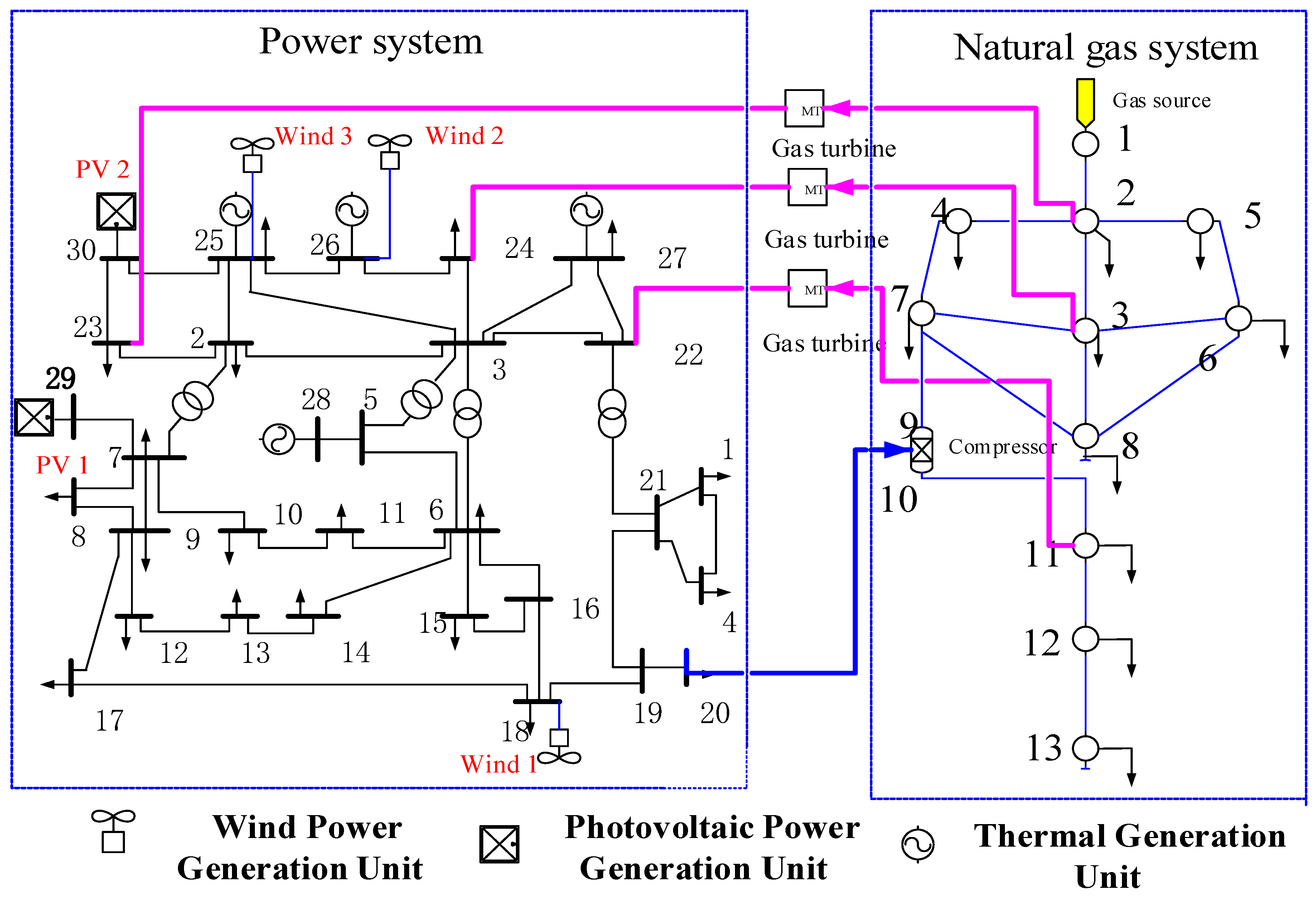
In this study, we simulated and analyzed the IES interconnected with an IEEE 30-bus power system and a 13-bus natural gas system. The overall diagram of the system is shown in Figure 2. There are three wind power plants and two solar power plants in the IES. The natural gas load at number 3 is a fluctuating load that satisfies the normal distribution. Specific data values for natural gas systems can be found in [1]. A gas turbine is equivalent to a power source in the power system and a load in the natural gas network. The conversion between input gas flow and output electric power is as follows:

$$H_{g,j}=a_{g,i}+b_{g,i}{P}_{G,i}+c_{g,i}{P}_{G,i}^2\begin{array}{cc}& j=2,3,11\begin{array}{cc}& i=23,24,22\end{array}\end{array},$$

(48)

$$F_{gas}^{m,j}=\frac{H_{g,i}}{GHV}\begin{array}{cc}& j=2,3,11\begin{array}{cc}& i=23,24,22\end{array}\end{array},$$

(49)

where $H_{g,\mathrm{j}}$ is the input heat value of gas turbine node $j$, $P_{G,i}$ is the output power of the gas turbine, $F_{gas}^{m,i}$ is the equivalent gas load of gas node $m$ in natural gas, $GHV$ is a fixed high calorific value ($GHV=0.2275$), and $a_{g,i}$, $b_{g,i}$, and $c_{g,i}$ are determined by the heat consumption curve of the gas turbine. In this case study, we simplify the heat consumption curve of the gas turbine and regard it as a linear relationship, that is, $a_{g,i}=0$, $b_{g,i}=7$, and $c_{g,i}=0$.

Hence, the relationship between the gas consumed by steam turbines and the electricity supplied to the power grid is as follows:

$$F_{gas}^{m,j}=30.76923\times P_{G,i}\begin{array}{cc}& \end{array}j=2,3,11\begin{array}{cc}& i=23,24,22\end{array}.$$

(50)

The compressor is equivalent to load for the power system, and its power consumption is as follows:

$$P_c^i=B{Q}_c[{(p_j^{}/p_m^{})}^k-1](\frac{0.7457}{{10}^5})\begin{array}{cc}& i=20\begin{array}{cc}& j=10\begin{array}{cc}& m=9\end{array}\end{array}\end{array},$$

(51)

where $P_c^i$ is the power consumed by compressors, $p_j^{}$ and $p_m^{}$ are the pressures of nodes $j$ and $m$, respectively, $Q_c$ is the gas flow rate from node $m$ to node $j$, $B$ is a coefficient ($B=306.2746$), $k$ is the compression ratio power, and $k=2$. Hence,

$$P_c^i=0.002284Q_c[{(p_j^{}/p_m^{})}^2-1]\begin{array}{cc}& i=20\begin{array}{cc}& j=10\begin{array}{cc}& m=9\end{array}\end{array}\end{array}.$$

(52)

5.1. Case 1: Estimation Points within the Limit Range

In this case, the mean of wind speed is 8.5 m/s, and each wind power plant follows the distribution given in Equation (9), where $k_p=2$, $c_p=10$, $x_{ci}=3.5\begin{array}{cc}& m/s\end{array}$, $x_{co}=18m/s$, $P=0.315MW$. Moreover, each photovoltaic power plant follows the distribution given in Equation (10), where $x$ is the standard light intensity value, $x=G_{stc}(t)/G_{stc\max }$, $\alpha =3$, $\beta =2$, $\frac{\Gamma (\alpha +\beta )}{\Gamma (\alpha )+\Gamma (\beta )}=20$, and $p_{}^{stc}=0.5MW$. The mean of the gas load 3 is $\mu =204m^3/h$, its standard deviation is $\delta =2$, We then have

$$f(v)=\frac{2}{10}(\frac{v}{10})e^{-{(\frac{v}{10})}^2}\begin{array}{cc}& v\ge 0\end{array},$$

(53)

$$h(v)=\{\begin{array}{cc}0& 0\le v<3.5\\ \frac{1}{46}(v-3.5)& 3.5\le v<18\\ 0.315& 18\le x\end{array},$$

(54)

$$f(x)=20{(x)}^2(1-x)\begin{array}{cc}& 0\le x\le \end{array}1.$$

(55)

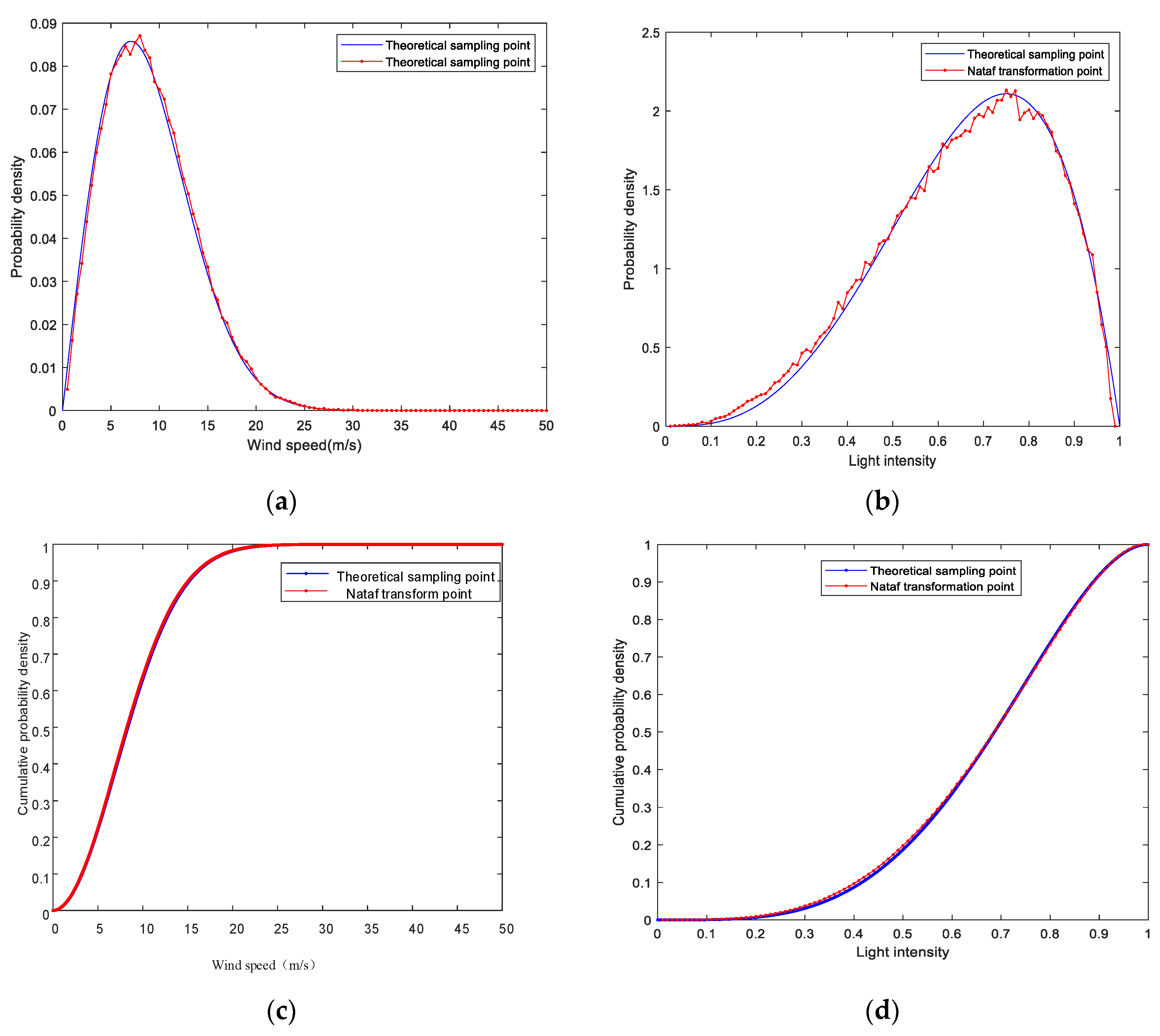
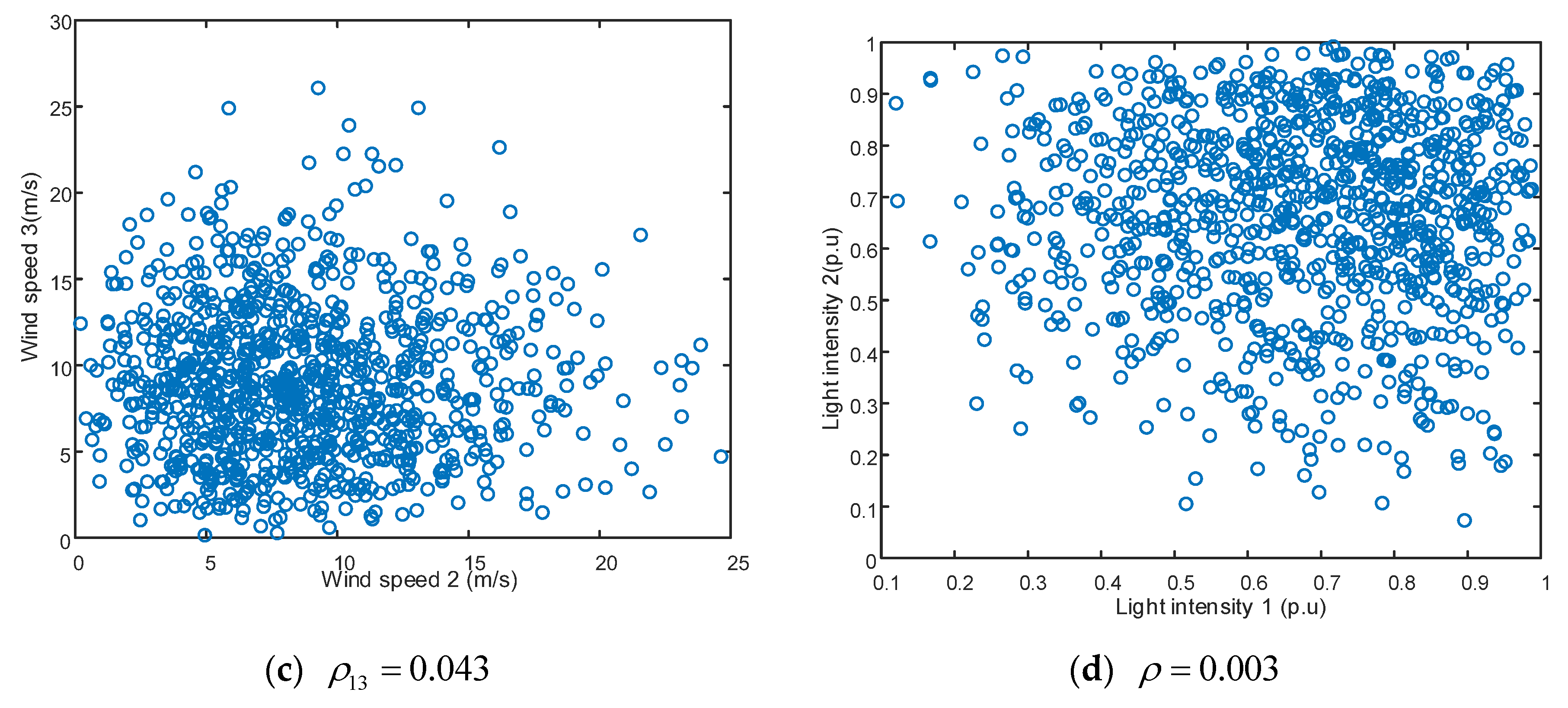
Figure 3 shows the probability density of the sampling points and probability distribution of the power plants and photovoltaic power plants after the Nataf transformation. The appearance of this figure noisy is because the pseudo random variables produced by the computer do not strictly satisfy the probability density function of samples. Figure 3c,d show that the results agree well the theoretical sampling points, indicating that the Nataf transformation has a very good precision.

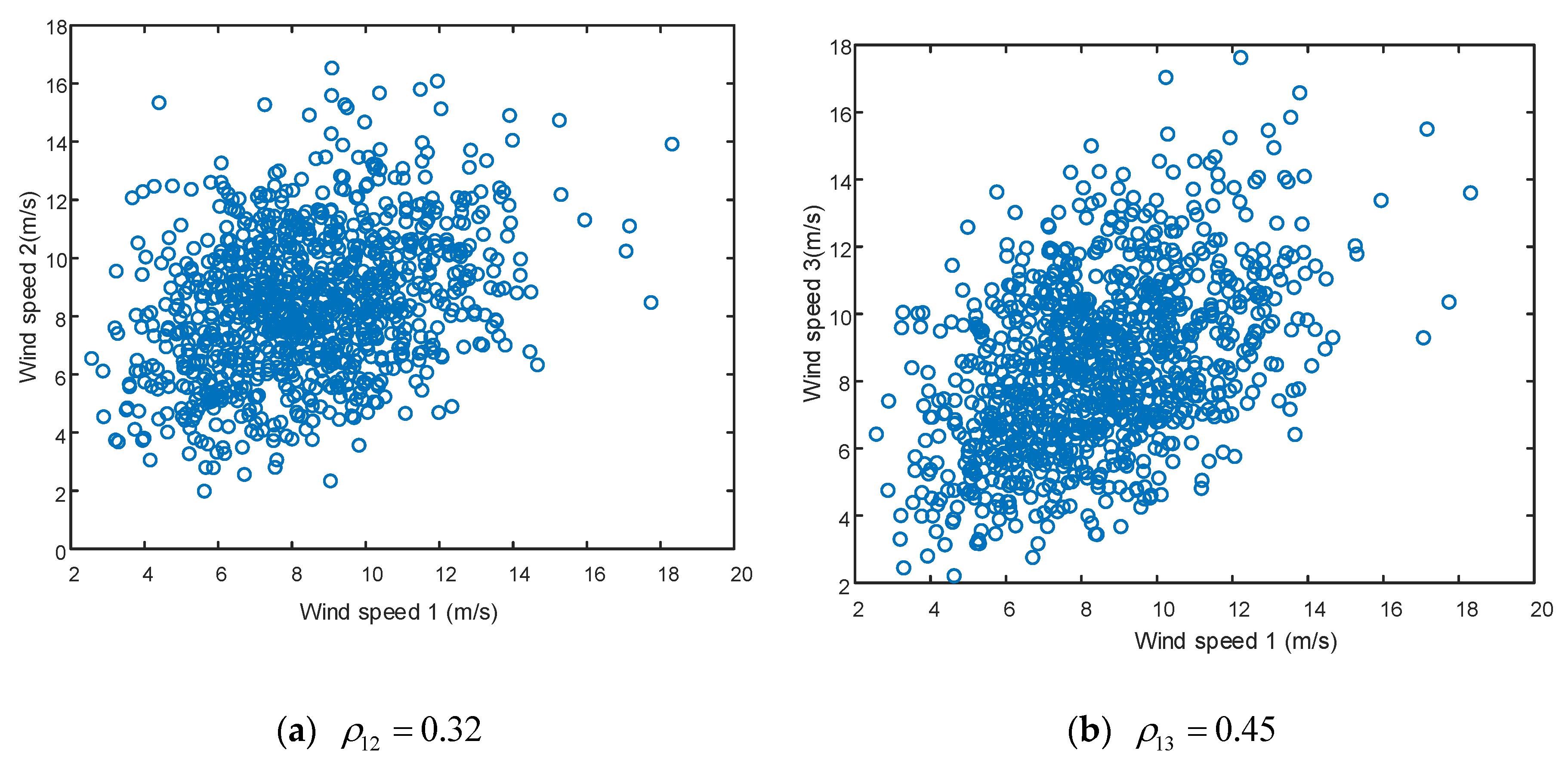
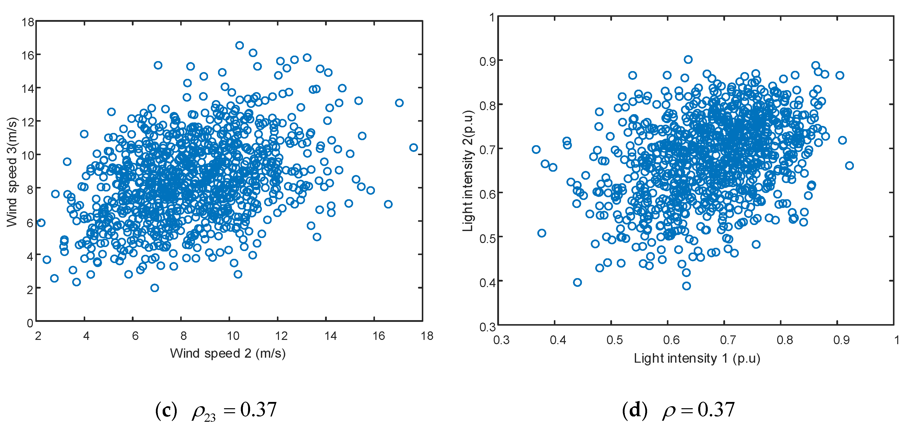
Figure 4 shows the correlation between each wind power plant and photovoltaic power plant after the Nataf transformation. The distribution of the sampling points is all concentrated in an ellipse. A flatter ellipse indicates a stronger correlation. It can be seen that the Nataf transformation controls the correlation well.

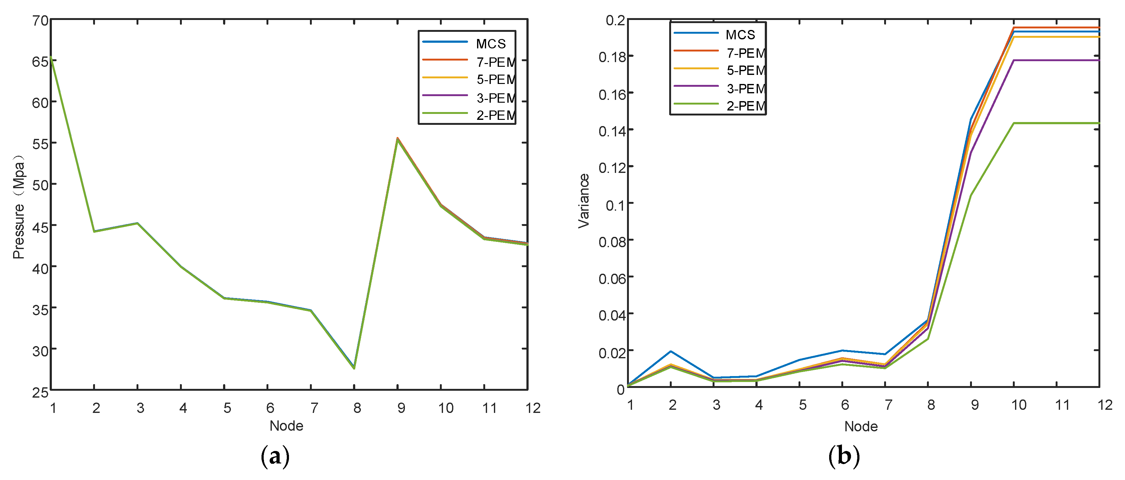
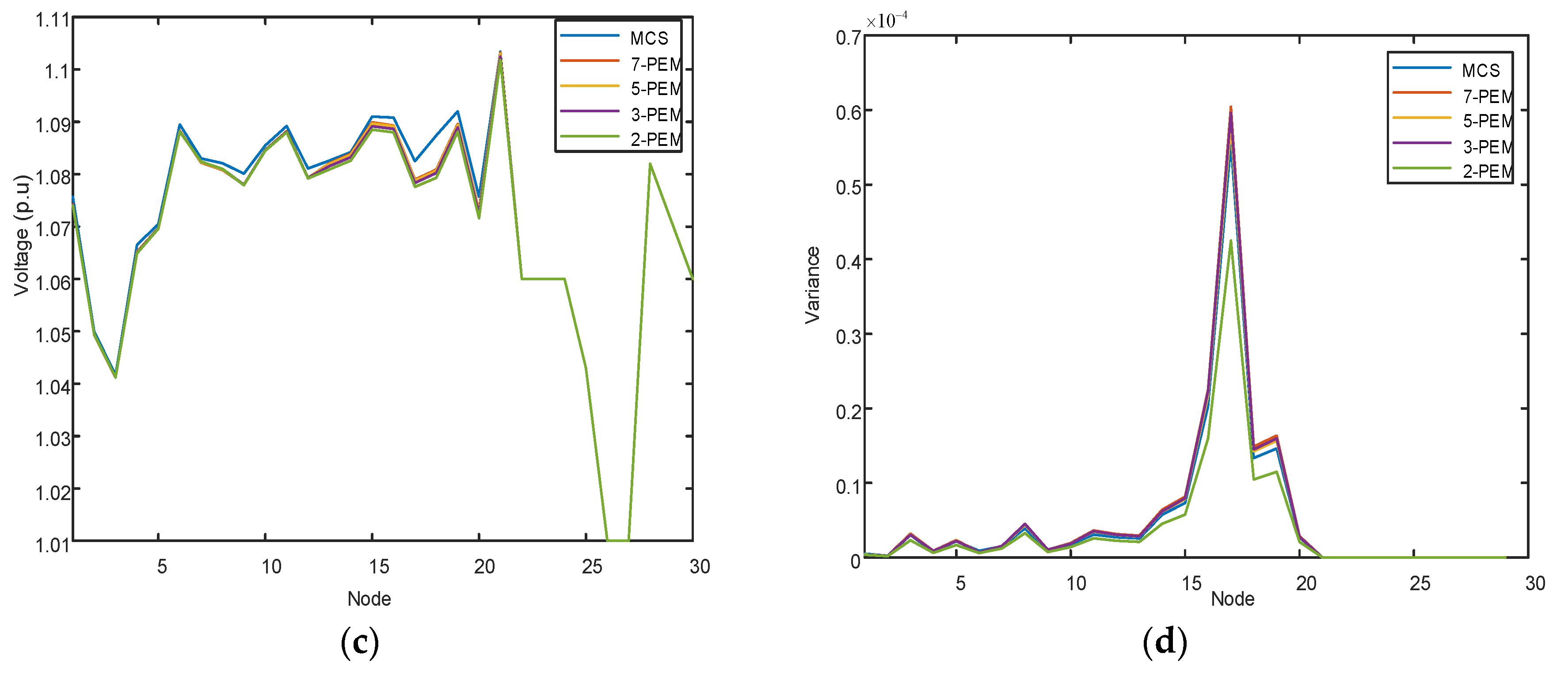
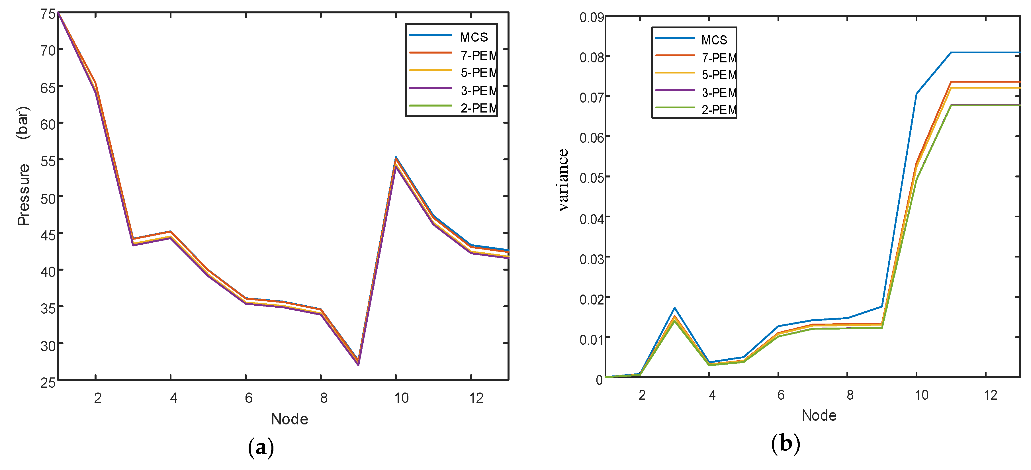
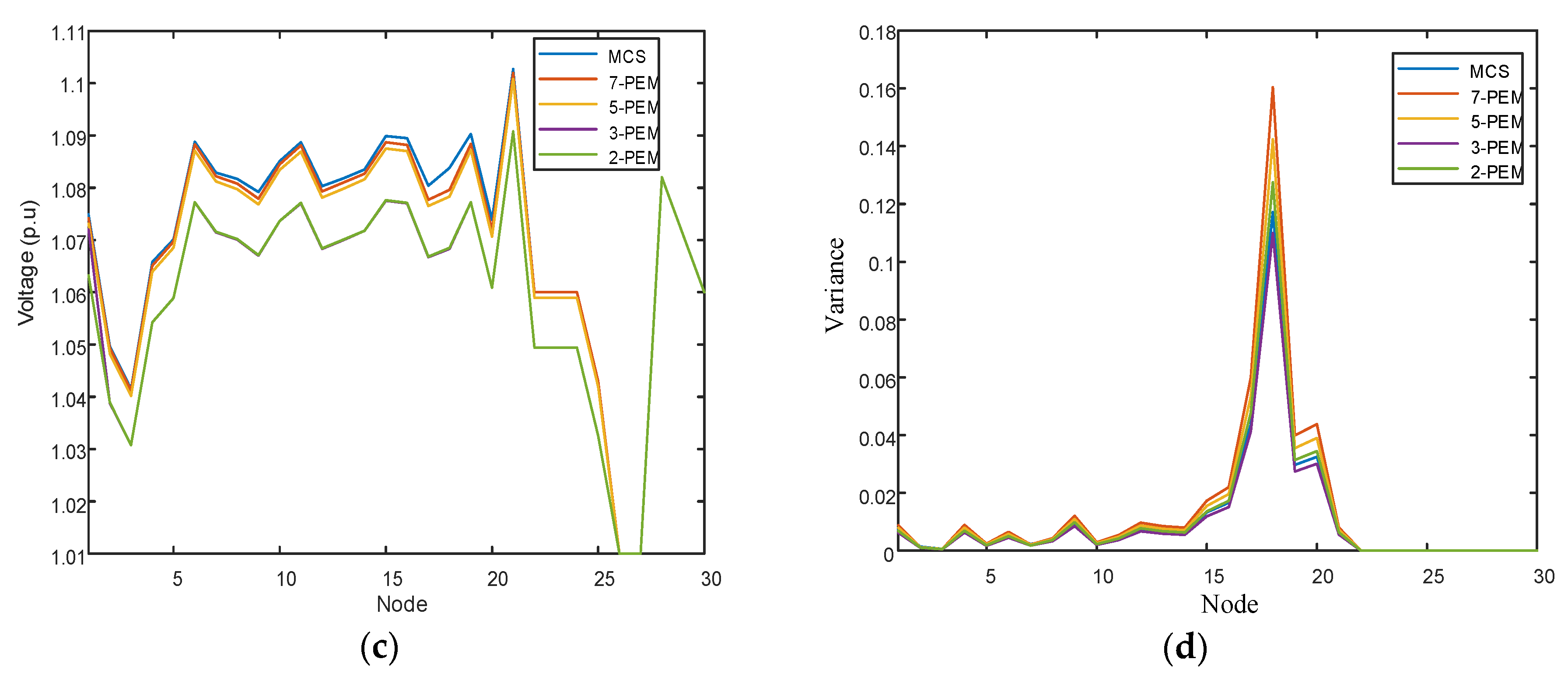
Next, these points are used to calculate the PEF. Figure 5 shows the results of m-PEM combined with the Nataf transformation. To show specific errors,

Table 2. Average relative error of the gas network.

Relative Error	7-PEM (%)	5-PEM (%)	3-PEM (%)	2-PEM (%)
mean	0.1164472	0.1725141	0.1930306	0.240743
variance	14.7833333	15.873716	21.8975776	25.6881084

and

Table 3. Average relative error of the power network.

Relative Error	7-PEM (%)	5-PEM (%)	3-PEM (%)	2-PEM (%)
mean	0.0999138	0.1050468	0.1179273	0.1408777
variance	3.3567948	3.251768	5.6100955	14.9320411

show the errors in the variance and mean. The calculation results show that this method has a very good accuracy when calculating the mean value, especially when calculating the mean value of the grid voltage. When calculating variance, it performs worse, which may be related to the number of Monte Carlo iterations. Because the PEF solution to an IES is very time-consuming, the number of Monte Carlo iterations must be as low as possible (3000). For 2-PEM, 3-PEM, 5-PEM, and 7-PEM, the computational quantities are 12, 18, 25, and 37, respectively.

To compare the results of PEF with and without the Nataf transformation, we used a common pseudo-random sample method for wind and photovoltaic farms. Figure 6 shows the correlation of common pseudo-random sampling points. It can be seen that the correlation of samples is very small: the correlation graph of the sample is approximately distributed in a circle in the plane. If the random error of sampling is ignored, the samples are independent of each other.

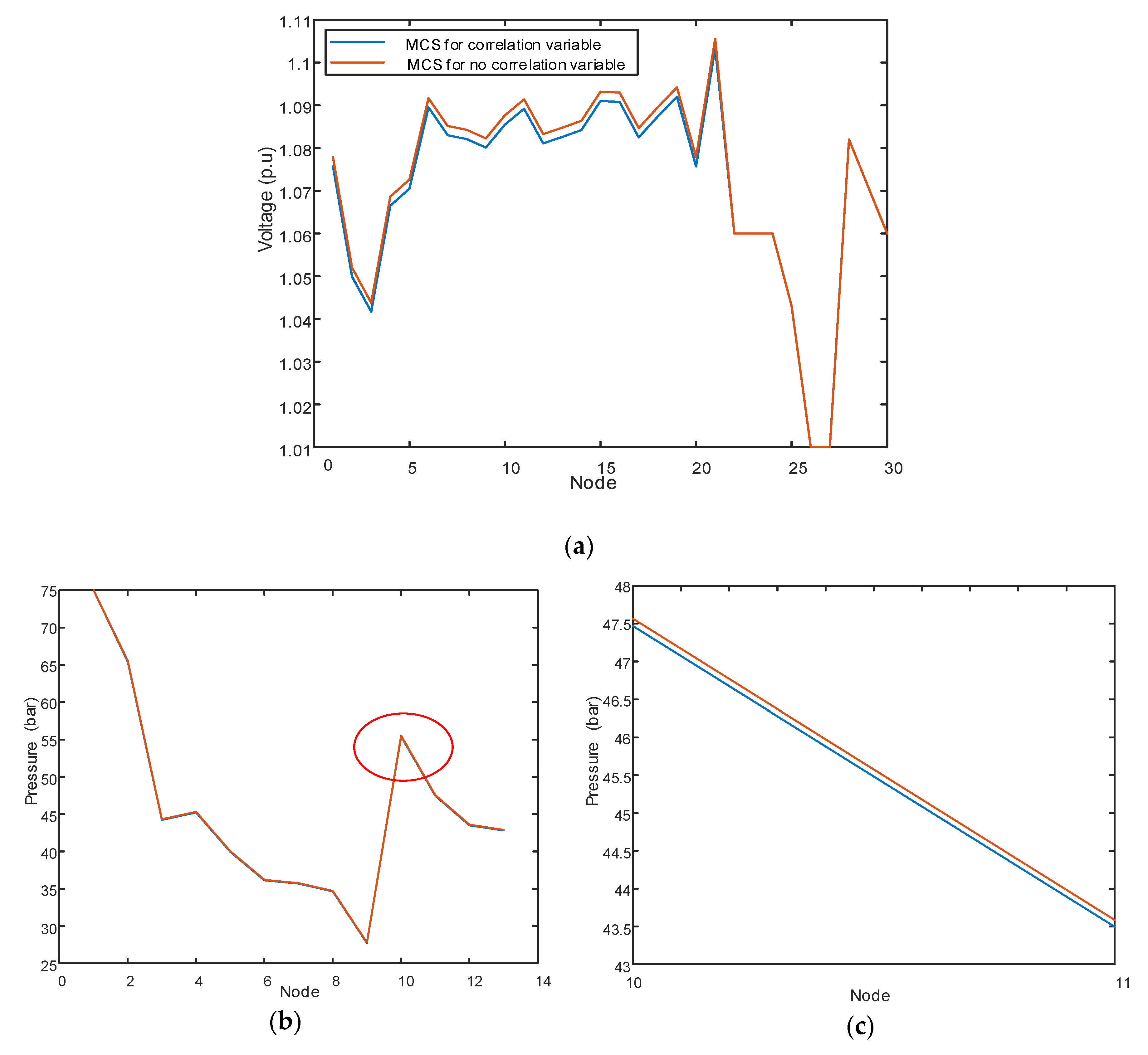
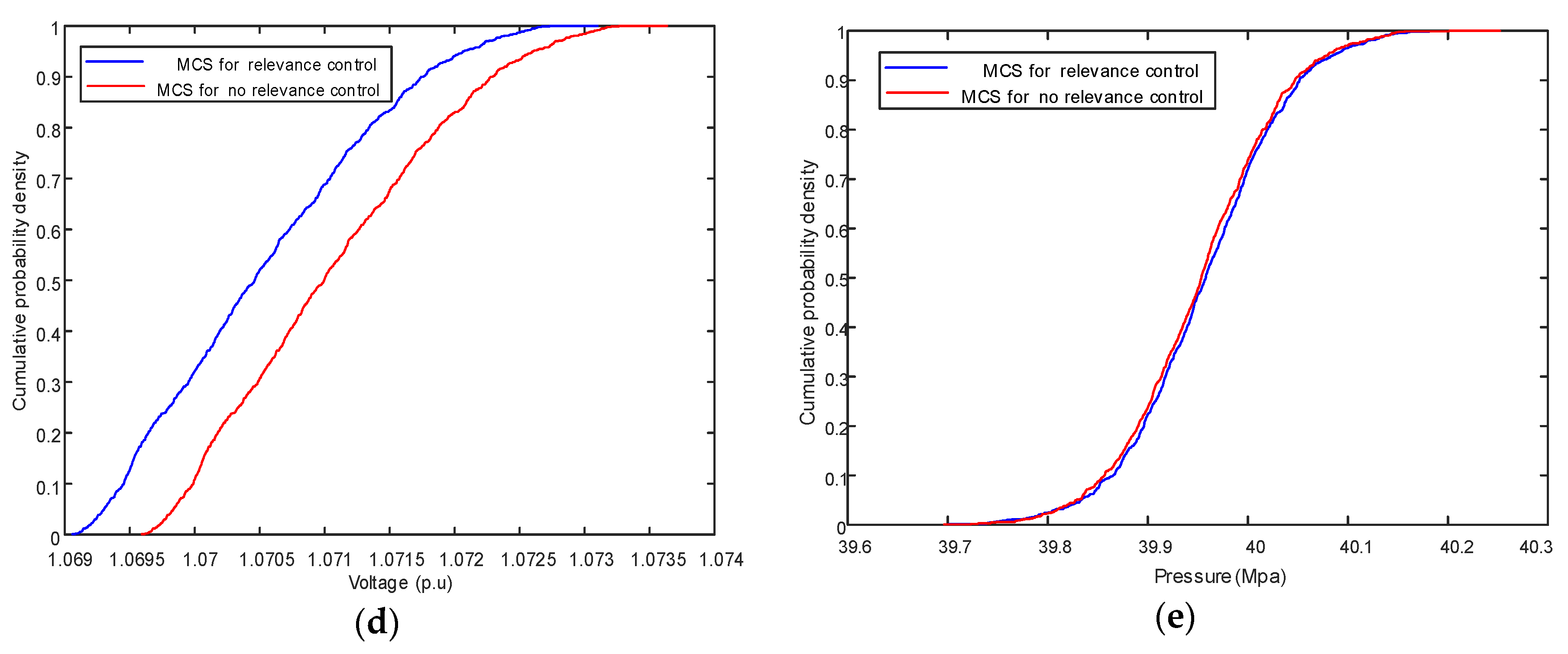
Next, the results of the two sampling methods were compared using MCS. Figure 7 shows the comparison results of MCS with and without the Nataf transformation. The effect of sampling without the Nataf transformation is even greater for the power system, because the correlation of the variables in this example is in the power network. The cumulative probability distributions of Figure 7d,e strongly support this point.

5.2. Case 2: Estimation Points Outside the Limits

In this case study, there is no wind in the environment, so the wind speed is lower than normal speed (mean = 7.14 m/s). Hence, the wind speed meets following conditions:

$$f(v)=(\frac{v}{32.5})e^{-{(\frac{v}{65})}^2}\begin{array}{cc}& v\ge 0\end{array},$$

(56)

$$h(v)=\{\begin{array}{cc}0& 0\le v<3.5\\ \frac{1}{46}(v-3.5)& 3.5\le v<18\\ 0.315& 18\le x\end{array},$$

(57)

where $k_p=2$, $c_p=65$, $x_{ci}=3.5m/s$, $x_{co}=18m/s$, $P=0.315MW$, and the photovoltaic data and gas load 3 are the same as those in Case 1.

Just as in Case 1, the relevance between each power plant and photovoltaic power plant is added using the Nataf transformation. Figure 8 shows the results of points that are outside of the boundary constraints, and

Table 4. Average relative error of the gas network.

Relative Error	7-PEM (%)	5-PEM (%)	3-PEM (%)	2-PEM (%)
mean	0.2399329	0.6347321	1.6014625	2.0714407
variance	13.499378	15.0755443	22.7094732	27.6881084

and

Table 5. Average relative error of the power network.

Relative Error	7-PEM (%)	5-PEM (%)	3-PEM (%)	2-PEM (%)
mean	0.0730304	0.1605961	0.8888845	0.9123241
variance	3.101779	7.9219449	8.9828336	17.1722688

show the errors in the variance and mean. It can be seen that the outside-of-range point has great impact on 2-PEM and 3-PEM. In these cases, the average error of the variance is more than 20%. The impacts on 5-PEM and 7-PEM are smaller.

For 2-PEM, 3-PEM, 5-PEM, and 7-PEM, the computation quantities are 12, 18, 25, and 37, respectively.

To limit points that are outside of the boundary constraints, the power transformation and equality constraints transformation methods are used to recalculate Case 2.

Table 6. Comparison of estimation points for different methods.

Method	Original Method	Power Transformation	Equality Constraint Transformation
2-PEM (m/s)	10.939	9.1205	9.0384
	3.351	5.3445	5.2664
3-PEM (m/s)	14.3745	invalid	10.285
	6.7123		4.0934
	1.6625		3.5

,

Table 7. Average relative error of gas network after constraining estimation points.

Relative Error	3-PEM(%)	2-PEM(%)
mean	/	0.8347321
variance	/	16.034543
(a) Power transformation method
Relative Error	3-PEM(%)	2-PEM(%)
mean	0.8222351	0.8123421
variance	14.983132	16.854671
(b) Equal constraint transformation method

and

Table 8. Average relative error of power network after constraining estimation points.

Relative Error	3-PEM(%)	2-PEM(%)
mean	/	0.2566954
variance	/	7.1256984
(a) Power transformation method
Relative Error	3-PEM(%)	2-PEM(%)
mean	0.8888845	0.9123241
variance	7.9845636	7.16879958
(b) Equal constraint transformation method

show the results of limiting the wind speed estimation points. It can be seen when the power transformation method works, the two methods have similar accuracy, but the equality constraint transformation method has wider applicability. In general, both methods effectively improve the accuracy of calculation.

6. Discussion

Liu presented a correlation coefficient transformation table for the Nataf transformation [30], which was convenient for Zhao and Ono’s MPEM. This study uses the work of these researchers to solve PEF. On the one hand, for 2-PEM and 3-PEM based on Zhao and Ono’s MPEM, estimated points outside of the range will cause a relatively large error. This study utilized the space conversion concept to overcome this limitation. The results show that spatial transformation is an important and effective method for solving PEF. One study [26] provided a good example of this transformation. Its aim was to link the probability space of an elliptic space with the probability space of the sample; the PPF was then solved. On the other hand, for 5-PEM and 7-PEM based on Zhao and Ono’s MPEM, direct calculations will lead to an exponential growth in the computation cost; therefore, we developed a modified MPEM.

Future research on probabilistic methods will focus more on accuracy and less on the cost of computation. As for the work discussed in this paper, the question as to whether 5-PEM and 7-PEM can allow estimation points outside the limit range without affecting accuracy is worth further investigation. In addition, combining PEF problems with economic dispatch, market operations, and optimization will also be directions for future research.

7. Conclusions

A PEM based on the Nataf transformation for computing PEF in an IES was proposed in this paper. This method is appropriate for large-scale electricity, gas, and thermal power interconnected systems because the energy flow calculations for such systems are complicated and time consuming; therefore, it is essential to reduce the cost of computation. From the results of the case studies, the following conclusions can be drawn:

• The proposed modified MPEM is effective in situations where the numbers of estimation points and variables are relatively large. The combination of the Nataf transformation with MPEM can obtain good accuracy. The proposed method makes the computational cost of m-PEM equal to that of (m − 1)-PEM, thus improving the computational efficiency.
• The power transformation and equality constraint transformation methods are used to reduce the large errors when the estimation points are outside of the boundary constraints. Simulation results show the effectiveness of the proposed methods.

Note that these methods are not only suitable for IESs but also for other scientific applications, such as the reliability analysis of structures and geotechnical reliability analysis.

References

1. Zhang, X.P.; Shahidehpour, M.; Alabdulwahab, A. Optimal expansion planning of energy hub with multiple energy infrastructures. IEEE Trans. Smart Grid 2015, 6, 2302–2311. [Google Scholar] [CrossRef]
2. Liu, C.; Shahidehpour, M.; Li, Z. Component & mode models for short-term scheduling of combined-cycle units. IEEE Trans. Power Syst. 2009, 24, 976–990. [Google Scholar]
3. Lu, B.; Shahidehpour, M. Short-term scheduling of combined-cycle units. IEEE Trans. Power Syst. 2004, 19, 1616–1625. [Google Scholar] [CrossRef]
4. Martinez-Mares, C.R. Fuerte-Esquivel. A unified gas and power flow analysis in natural gas and electricity coupled networks. IEEE Trans. Power Syst. 2012, 27, 2156–2166. [Google Scholar] [CrossRef]
5. Barati, F.; Seifi, H.; Sepasian, M.S. Multi-period integrated framework of generation, transmission, and natural gas grid expansion planning for large-scale systems. IEEE Trans. Power Syst. 2015, 30, 2527–2537. [Google Scholar] [CrossRef]
6. Spiecker, S. Modeling market power by natural gas producers and its impact on the power system. IEEE Trans. Power Syst. 2013, 28, 3737–3746. [Google Scholar] [CrossRef]
7. Rehmani, M.H.G.; Reisslein, M.G.; Rachedi, A.; Erol-Kantarci, M.G. Integrating renewable energy resources into the smart grid: Recent developments in information and communication technologies. IEEE Trans. Ind. Inform. 2018, 14, 2814–2825. [Google Scholar] [CrossRef]
8. Liu, N.; Wang, J.; Wang, L. Hybrid Energy Sharing for Multiple Microgrids in an Integrated Heat–Electricity Energy System. IEEE Trans. Sustain. Energy 2019, 10, 1139–1151. [Google Scholar] [CrossRef]
9. Chen, S.; Wei, Z.; Sun, G. Multi-Linear Probabilistic Energy Flow Analysis of Integrated Electrical and Natural-Gas Systems. IEEE Trans. Power Syst. 2017, 32, 1970–1979. [Google Scholar] [CrossRef]
10. Abeysekera, M.; Wu, J.; Jenkins, N. Steady state analysis of gas networks with distributed injection of alternative gas. Appl. Energy 2015, 164, 991–1002. [Google Scholar] [CrossRef]
11. Zhang, P.; Lee, S.T. Probabilistic load flow computation using the method of combined cumulants and Gram-Charlier expansion. IEEE Trans. Power Syst. 2004, 19, 676–682. [Google Scholar] [CrossRef]
12. Chaudry, M.; Wu, J.Z. A sequential Monte Carlo model of the combined GB gas and electricity network. Energy Policy 2013, 62, 473–483. [Google Scholar] [CrossRef]
13. Martinez-Mares, C.R. Fuerte-Esquivel. A robust optimization approach for the interdependency analysis of integrated energy systems considering wind power uncertainty. IEEE Trans. Power Syst. 2013, 28, 3964–3976. [Google Scholar] [CrossRef]
14. Ghanem, R.G.; Spanos, P.D. Stochastic Finite Elements: A Spectral Approach; Springer: Berlin, Germany, 1991. [Google Scholar]
15. Alipour, M.; Zare, K. MINLP Probabilistic Scheduling Model for Demand Response Programs Integrated Energy Hubs. IEEE Trans. Ind. Inform. 2018, 14, 79–88. [Google Scholar] [CrossRef]
16. Oliverira, G.C.; Pereira, M.V.F. A Technique for Reduced Computational Effort in Monte Carlo Based Composite Reliability Evaluation. IEEE Trans. Power Syst. 1989, 4, 1309–1315. [Google Scholar] [CrossRef]
17. Yu, H.; Chung, C.Y.; Wong, K.P. Probabilistic Load Flow Evaluation with Hybrid Latin Hypercube Sampling and Cholesky Decomposition. IEEE Trans. Power Syst. 2009, 20, 661–667. [Google Scholar] [CrossRef]
18. Cunha, S.H.F.; Pereira, M.V.F.; Oliverira, G.C. Composite Generation and Transmission Reliability Evaluation Large Scale Hydroelectric Power Systems. IEEE Trans. Appar. Syst. 1985, 104, 2657–2663. [Google Scholar] [CrossRef]
19. Wei, Z.K.; Xu, J.F.; Dai, X.K. Research on Coarse-Grained Parallel Algorithm of the Monte-Carlo Simulation for Probabilistic Load flow Calculation. In Proceedings of the International Conference on Power and Energy (CPE 2014), Shanghai, China, 3–29 November 2014. [Google Scholar]
20. Xie, Z.Q.; Ji, T.Y.; Li, M.S. Quasi-Monte Carlo Based Probabilistic Optimal Power Flow Considering the Correlation of Wind Speeds Using Copula Function. IEEE Trans. Power Syst. 2018, 33, 2239–2247. [Google Scholar] [CrossRef]
21. Wang, C.; Qiu, Z.; Yang, Y. Uncertainty propagation of heat conduction problem with multiple random inputs. Int. J. Heat Mass Transf. 2016, 99, 95101. [Google Scholar] [CrossRef]
22. Xu, Y.; Mili, L.; Sandu, A. Propagating Uncertainty in Power System Dynamic Simulations Using Polynomial Chaos. IEEE Trans. Power Syst. 2019, 34, 338–348. [Google Scholar] [CrossRef]
23. Zhang, Y.; Hosder, S. Robust Design Optimization Under Mixed Uncertainties with Stochastic Expansions. J. Mech. Des. 2013, 135, 81005. [Google Scholar] [CrossRef]
24. Li, X.; Li, Y.Z.; H, S. Zhang, Analysis of Probabilistic Optimal Power Flow Taking Account of the Variation of Load Power. IEEE Trans. Power Syst. 2008, 23, 992–999. [Google Scholar]
25. Morates, J.M.; Ruiz, J.P. Point estimate schemes to solve the probabilistic power flow. IEEE Trans. Power Syst. 2007, 22, 1594–1601. [Google Scholar] [CrossRef]
26. Aien, M.; Fotuhi-Firuzabad, M.; Aminifar, F. Probabilistic Load Flow in Correlated Uncertain Environment Using Unscented Transformation. IEEE Trans. Power Syst. 2012, 27, 2233–2241. [Google Scholar] [CrossRef]
27. Huang, Y.; Xu, Q.; Yang, Y. Numerical method for probabilistic load flow computation with multiple correlated random variables. IET Renew. Power Gener. 2018, 12, 1295–1303. [Google Scholar] [CrossRef]
28. Chen, X.; Tung, Y.K. Investigation of polynomial normal transform. Struct. Saf. 2003, 25, 423–445. [Google Scholar] [CrossRef]
29. Morales, J.M.; Baringo, L.; Conejo, A.J.; Mnguez, R. Probabilistic power flow with correlated wind sources. IET Gener. Transm. Distrib. 2010, 4, 641–651. [Google Scholar] [CrossRef] [Green Version]
30. Liu, P.L.; Der Kiureghian, A. Multivariate distribution models with prescribed marginals and covariances. Probab. Eng. Mech. 1986, 1, 105–112. [Google Scholar] [CrossRef]
31. Xie, X.; Krewer, U.; Schenkendorf, R. Robust optimization of dynamical systems with correlated random variables using the point estimate method. IFAC-Pap. Online 2018, 51, 427–432. [Google Scholar] [CrossRef]
32. Hong, H.P. An efficient point estimate method for probabilistic analysis. Reliab. Eng. Syst. Saf. 1998, 8, 261–267. [Google Scholar] [CrossRef]
33. Zhao, Y.G.; Ono, T. New point estimates for probability moments. J. Eng. Mech. 2000, 126, 433–436. [Google Scholar] [CrossRef]
34. Su, C.L. Probabilistic load-flow computation using point estimate method. IEEE Trans. Power Syst. 2005, 20, 1843–1851. [Google Scholar] [CrossRef]
35. Kloubert, M.L.; Rehtanz, C. Enhancement to the Combination of Pointestimate Method and Gram–Charlier Expansion Method for Probabilistic load Flow Computations; Power Tech: Manchester, UK, 2017; pp. 1–6. [Google Scholar]
Figure 1. Steady-state energy flow calculation in an integrated energy systems.
Applsci 09 03291 g001
Figure 2. Diagram of the IES used in the case study.
Applsci 09 03291 g002
Figure 3. Probability density of sampling points in (a) wind power plants and (b) photovoltaic power plants. Cumulative probability distribution of (c) wind power plants and (d) photovoltaic power plants.
Applsci 09 03291 g003
Figure 4. Results for point estimate method with the Nataf transformation for Case 1. Correlations in the wind speeds of (a) wind power plants 1 and 2, (b) wind power plants 1 and 3, and (c) wind power plants 2 and 3. (d) Correlation in the light intensity for the photovoltaic power plants.
Applsci 09 03291 g004aApplsci 09 03291 g004b
Figure 5. Case 1 results. (a) Mean pressure for the natural gas network. (b) Variance in pressure for the natural gas network. (c) Mean voltage for the power network. (d) Variance in voltage for the power network.
Applsci 09 03291 g005aApplsci 09 03291 g005b
Figure 6. Results for PEM without the Nataf transformation for Case 1. Correlations in the wind speeds of (a) wind power plants 1 and 2, (b) wind power plants 1 and 3, (c) wind power plants 2 and 3, and (d) photovoltaic power plants.
Applsci 09 03291 g006aApplsci 09 03291 g006b
Figure 7. Comparison of Monte Carlo results with and without the Nataf transformation for Case 1. (a) Voltage results for each node. (b) Mean pressure for the natural gas network. (c) Enlargement of key points. (d) Cumulative probability of node 5 in the power network. (e) Cumulative probability of node 5 in the gas network.
Applsci 09 03291 g007aApplsci 09 03291 g007b
Figure 8. Case 2 results. (a) Mean pressure for the natural gas network. (b) Variance in pressure for the natural gas network. (c) Mean pressure for the power network. (d) Variance in pressure for the power network.
Applsci 09 03291 g008aApplsci 09 03291 g008b