Abstract
Long-distance oil and gas pipelines are inevitably impacted by rockfalls during geologic hazards such as mud-rock flow and landslides, which have a serious effect on the safe operation of pipelines. In view of this, an experimental and numerical study on the strain behavior of buried pipelines under the impact load of rockfall was developed. The impact load exerted on the soil, and the strains of buried pipeline caused by the impact load were theoretically derived. A scale model experiment was conducted using a self-designed soil-box to simulate the complex geological conditions of the buried pipeline. The simulation model of hammer–soil–pipeline was established to investigate the dynamic response of the buried pipeline. Based on the theoretical, experimental, and finite element analysis (FEA) results, the overall strain behavior of the buried pipeline was obtained and the effects of parameters on the strain developments of the pipelines were analyzed. Research results show that the theoretical calculation results of the impact load and the peak strain were in good agreement with the experimental and FEA results, which indicates that the mathematical formula and the finite element models are accurate for the prediction of pipeline response under the impact load. In addition, decreasing the diameter, as well as increasing the wall thickness of the pipeline and the buried depth above the pipeline, could improve the ability of the pipeline to resist the impact load. These results could provide a reference for seismic design of pipelines in engineering.
1. Introduction
Under complex geological conditions such as mud-rock flow and landslides, long-distance oil and gas pipelines are inevitably impacted by rockfalls, seriously resulting in pipeline corrosion, cracking, deformation, and other damages [1,2,3,4]. The serious structural damages of buried pipelines caused by rockfalls attracted much attention from engineers and researchers in recent years. In addition, with the recent rapid development of damage detection and structural health monitoring technology [5,6,7], the monitoring technology of buried pipelines was also developed and it plays an important role in the safe operation of pipeline network systems. In order to further analyze the damage mechanism of buried pipelines, it is necessary to conduct experimental and numerical studies on the strain behavior of buried pipelines subjected to impact loads for the safe operation of pipelines, as well as for loss prevention and environmental protection.
In recent years, many researches on buried pipelines under impact loads mainly focused on finite element analysis (FEA) and the theoretical derivation. Among them, three main calculation modes in FEA were applied to investigate the buried pipelines, including the beam mode [8,9], the shell mode [10,11], and the beam–shell mode [12]. Compared to the beam mode, the shell mode is widely used in FEA due to the more accurate results in calculating the distribution of the large deformation of pipelines. Liu et al. [13] applied the shell mode to simulate the large deformation section of a pipeline under fault movement and concluded that the shell mode could clearly analyze the local buckling and the large deformation of pipeline, but this model had no consideration of the effect of soil property when calculating the sliding friction of pipeline–soil. For further research, Zhang et al. [14] and Liu et al. [15] established the soil–pipeline model in FEA, and completely studied the effects of different parameters (the initial defects, the impact energy, the pipeline wall thickness, the buried depth of pipeline, and the soil properties) on the strain behavior of buried pipelines under impact loads. Furthermore, thorough research on the cross-section deformation and the soil pressure on the pipeline during the impact process was carried out by Deng et al. [16] through the three-dimensional distinct element code software. The results indicated that the main factors affecting the cross-section deformation of the pipeline were the impact velocity and the mass of rockfall. Alongside finite element research, theoretical researches on buried pipelines under impact loads were more comprehensive. Among them, the theoretical researches mainly focused on the theoretical calculation of the impact force on soil and the earth pressure on pipelines. The impact of rockfall can be simplified to a low-speed collision problem in engineering practice. There are three main theoretical methods for calculating the impact force on soil: the Hertz collision theory [17,18,19], the energy theory, and the inelastic collision method [20]. In the former two methods, rockfall and soil are regarded as elastic bodies, unlike the impact force on soil in actual working conditions. The latter method is more reasonable for the consideration of the energy loss, while the calculation process is more complicated. Subsequently, Qi et al. [21] developed a new mathematical model of the impact force from rockfalls to obtain the wallop amplification coefficient, but some differences still existed between the actual situation and the theoretical conditions. Moreover, Ye et al. [22] also studied a new method for calculating the impact force of the rockfall with the consideration of the rockfall weight and the rebound effect, and they validated the feasibility of the proposed calculation method of impact force using examples. For the theoretical calculation of earth pressure on pipelines, a variety of calculation methods of earth pressure were reasonably applied in practical projects, i.e., the Marston method [23,24] based on the limit equilibrium theory, the Hindy method [25], and the empirical coefficient method of earth pressure [26,27,28]. At present, the calculation method of earth pressure is commonly based on the Marston method. Moreover, Yun and Kang [29] carried out research on the mechanical model of pipelines in landslide conditions and calculated the stress distribution on pipelines using the theory of Winkler. For further research, the safety factor equation of pipelines subjected to impact force was summarized. Jing et al. [30] analyzed the dynamic response of buried pipelines impacted by rockfalls by combining the theoretical calculation formula and LS-DYNA. The results showed that there was an approximate proportional relationship between the maximum impact force and velocity; the stress concentration existed on the upper and lower surfaces of the pipeline, and the vertical stress distributed along the longitudinal and transversal directions of the pipeline; then, it decreased gradually along both ends of the pipeline.
Although the finite element analysis (FEA) of and theoretical research on buried pipelines impacted by rockfalls were conducted by many scholars in the past, the experimental investigation of buried pipelines under impact loads was absent due to the complexity of the non-linear contact problem and the difficulty of full-scale experiments. Furthermore, the effects of pipeline parameters on the strain behavior of buried pipelines under impact loads need to be further explored by combining theoretical derivation, experimental research, and FEA. Therefore, an experimental and numerical study on the strain behavior of a buried pipeline subjected to an impact load was established in this research through theoretical research, experimental study, and simulation. The purposes of this research were threefold. Firstly, the rockfall impact force on soil, and the loads and strains on a buried pipeline under an impact load were theoretically derived based on the Hertz collision theory and the Spangler formula. Secondly, a soil-box was designed to conduct a scale experiment of 10 buried pipelines under impact load using a drop hammer impact test machine. Thirdly, an FEA model of hammer–soil–pipeline was developed for further investigation of the dynamic response of the buried pipeline under an impact load, and its accuracy was verified by theoretical and experimental results. Finally, the effect of some important parameters (the wall thickness of the pipeline, the diameter of the pipeline, the buried depth, and the impact height) on the strain behavior of the buried pipeline under an impact load was discussed based on the theoretical, experimental, and FEA results.
2. Theoretical Research
2.1. The Rockfall Impact Force on Soil
For buried pipelines under impact loads from rockfalls, the mathematical formula for calculating the impact force on the soil can be derived. When the rockfall impacts the soil (pebble or clay) with a certain speed, it may sink to a certain depth and the velocity rapidly decreases. During this process, because the stiffness of the soil is smaller than that of the rockfall, the rockfall generally does not rebound slightly and, furthermore, the impact process is very short, which causes a larger impact force. The physical model of a buried long pipeline under a rockfall impact load can be simplified as shown in Figure 1, and the curve of the impact force (F) versus time (t) during this impact process is shown in Figure 2 based on the Hertz collision theory and relevant references [31], in which Fmax is the maximum impact force and t1 is time when F reaches to Fmax.
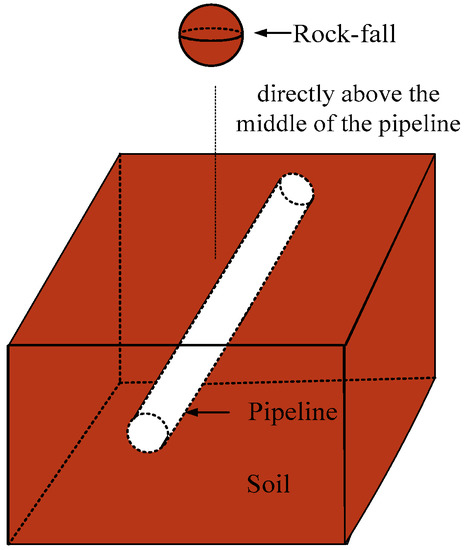
Figure 1.
The physical model of a buried long pipeline under an impact load.
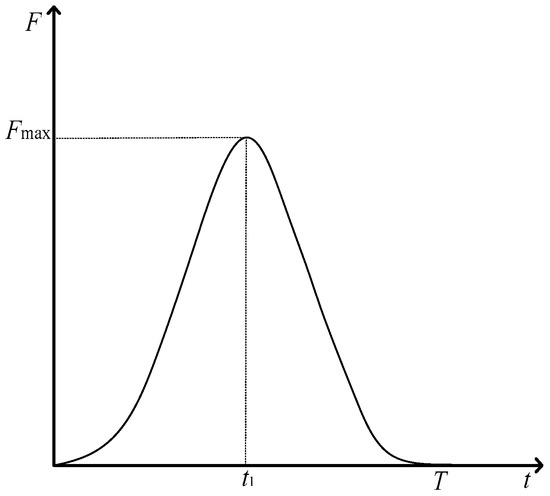
Figure 2.
Impact force (F) versus time (t) curve.
Three main calculation methods of Fmax are the Hertz collision theory, the energy theory, and the inelastic collision method. The velocity of rockfall may not be perpendicular to the soil, but this experiment mainly focuses on the case where the rockfall impacts the soil vertically based on the Hertz collision theory. It is essential for the Hertz collision theory to make the following assumptions: (1) the rockfall is a rigid body where no deformation occurs during the collision; (2) the rockfall is not separated from the soil during the collision, and the friction between them is not considered; (3) based on a linear elastic half-space theory, the maximum displacement of the soil is in the elastic stage; (4) only the first impulse action is taken into consideration. Based on the above assumptions, the motion equation of Fmax on soil can be written as follows:
where m1 and m2 are the masses of the two elastic spheres (rockfall and soil), is the instantaneous velocity before the collision, and K is a stiffness coefficient determined by the following equations:
where r1 and r2 are the radii of the two elastic spheres (rockfall and soil), E1 and E2 are the elastic moduli of the two elastic spheres, and μ1 and μ2 are the Poisson ratios of the two elastic spheres. When the rockfall impacts the soil, it can be considered that E1 approaches infinity since the stiffness of the rockfall is much larger than that of the soil. The values of m2 and r2 approach infinity since the soil is regarded as a semi-linear elastomer. Therefore, the following equations can be derived:
Substituting Equation (6) into Equation (1) gives Fmax as
where , and is the density of the rockfall. Assuming that the pressure on the contact surface between the rockfall and the soil is uniformly distributed, then the impact pressure () can be expressed as
where A represents the contact area between the rockfall and the soil.
2.2. The Loads on a Buried Long Pipeline
2.2.1. The Vertical Compressive Load
The total vertical compression on the pipeline (P) consists of the pressure from the rockfall impact force transmitting through the soil above the pipeline () and the earth pressure above the pipeline (Pv), depicted as follows [32]:
where f represents the penetration coefficient which is related to the buried depth from the soil surface to the crown of the pipeline, as shown in Table 1.

Table 1.
The relationship between the buried depth of the pipeline and .
In a collision, the contact area between the rockfall and the soil is smaller than the surface of the soil and, furthermore, the length of the pipeline is relatively infinite; thus, Fmax can be regarded as a vertical concentrated load that can be calculated by Equation (7), and its sketch is depicted in Figure 3, in which Fmax is the vertical concentrated load which acts on the coordinate origin.
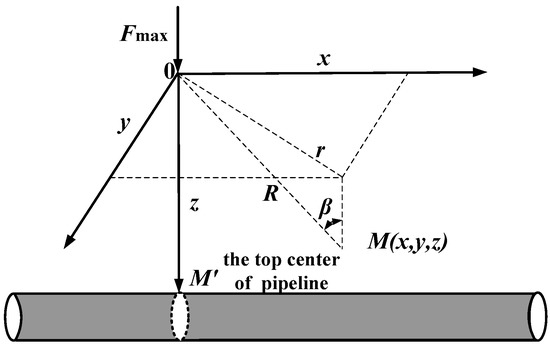
Figure 3.
Vertical concentrated load of the soil layer.
The vertical pressure () at a certain position in the soil, i.e., point M as shown in Figure 3, can be expressed as follows [33]:
where R is the distance between point M and the original coordinate shown as follows:
In Figure 3, β is the angle between the depth (z) and the distance (R), which can be obtained by the following equation:
When the pressure acting on point M’ of the buried pipeline reaches up to Fmax, y approximates to 0. Therefore, the following equation can be obtained:
Substituting Equations (12) and (13) into Equation (10), we can obtain the pressure from the rockfall impact force transmitting through the soil above the pipeline as shown below.
The calculation method of the earth pressure of the soil above the pipeline exerted on the pipeline can be divided into two cases based on the position of water line. When the groundwater level is under the pipeline, Pv is a constant load generated by the gravity of the soil, and can be represented as follows [34]:
where is the unit weight of the soil, while C1 is the buried depth of pipeline.
When the groundwater level is over the pipeline, the buoyancy effect of water should be taken into account. The Pv can then be expressed as follows:
where C2, , , and denote the height between the ground surface and the groundwater level, the saturated unit weight of the soil, the unit weight of water, and the height of the groundwater level over the crown of the pipeline, respectively.
2.2.2. The Horizontal Load
The horizontal load exerted on the pipeline (qx) can be calculated through the vertical load from the rockfall impact force (), as shown below.
where λ represents the horizontal pressure coefficient of the soil, , and is the internal friction coefficient of the soil.
2.3. The Strains on a Buried Long Pipeline
As shown in Figure 4, the deformation of a pipeline can be calculated using the Code for Design of Oil Transportation Pipeline Engineering (GB50253-2003) [35] and the Spangler Formula [36,37].
where , D, , K, E, I, R, E’, and T denote the deformation of the pipeline, the outside diameter of the pipeline, the deformation hysteresis coefficient which is taken as 1.5, the base coefficient of a steel pipeline, the elasticity modulus of the pipeline, the moment of inertia of the pipeline, the radius of the pipeline, the elasticity modulus of the soil, and the wall thickness of pipeline, respectively. P represents the total vertical load on the unit length of the pipeline and can be expressed by Equation (9).
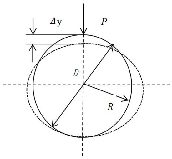
Figure 4.
The deformation of the pipeline.
The stress distribution of the pipeline on the entire section is shown in Figure 5. The maximum stress on the cross-section of the pipeline, , can be obtained as follows:
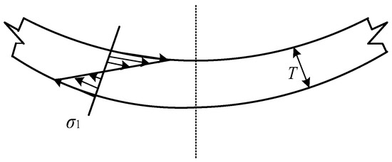
Figure 5.
The stress distribution of the pipeline.
Finally, the maximum strain on the cross-section of pipeline can be expressed as
3. Experimental Program
3.1. Experimental Design
In practical engineering, the buried depth of a pipeline is generally 2.5 m with a diameter of 700 mm; moreover, the effective length of a buried pipeline is generally 20 m. In view of the Technical Specification for Seismic Resistance of Oil and Gas Pipeline Engineering and relevant literature [38,39,40], a scale of the specimens was taken as 1:7 to simulate the actual pipeline in this test. Table 2 shows the cross-sectional dimensions and the impact parameters of all specimens without consideration of the effect of oil and gas pressure. As shown in Table 2, all specimens were labeled to identify the diameter, thickness, buried depth, and impact height of the specimens. For example, the label “A114 × 2.5-d0.6-H0.5” is defined as follows:
Table 2.
Details of specimens.
The first part “A” represents that the specimen is in group A.
The second part “114 × 2.5” indicates that the specimen has a diameter (D) of 114 mm and a thickness (T) of 2.5 mm.
The third part “d0.6” means that the buried depth (d) of the specimen is 0.6 m.
The last part “H0.5” denotes that the impact height of the drop hammer (H) is 0.5 m.
The size of the soil-box for laying the soil and pipeline was 3.0 m (length) × 3.0 m (width) × 1.5 m (height), which was welded by a steel plate, channel steel, and angle steel, as shown in Figure 6.
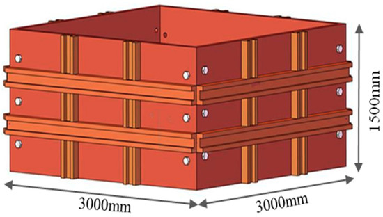
Figure 6.
The schematic of the soil-box.
3.2. Material Property
Clay, commonly applied in practical engineering, was adopted as the soil. By sampling the compacted soil, the material parameters of the soil were measured as shown in Table 3. The pipeline was fabricated from Chinese Standard Q235 galvanized steel (nominal yield stress fy,k = 235 MPa). A tensile test was carried out on the pipeline, and the mechanical properties were measured as shown in Table 4.
Table 3.
Mechanical properties of the soil.
Table 4.
Mechanical properties of the pipelines.
3.3. Layout of Measuring Points
The strain gauges (2 mm × 1 mm) were adopted to measure the longitudinal and transversal strains of the buried pipelines, as shown in Figure 7. The strain acquisition system was the Wireless Dynamic Strain Collector DH5908, as shown in Figure 8. The strain gauges were linked to the wireless transmitter terminal of the acquisition system. There are three channels on the DH5908. Channels A–A and C–C were both reserved for the four strain gauges located one-fourth of the member length from both sides of the pipeline. Meanwhile, channel B–B was reserved for the four strain gauges located in the mid-span of the pipeline. In addition, the accelerometer INV9822A was installed on the drop hammer, and the output signal was recorded by the acquisition instrument INV3018, as shown in Figure 8b.
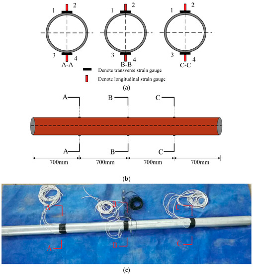
Figure 7.
Layout of strain gauge: (a) section of pipeline; (b) schematic of pipeline strain measurement point; (c) photograph of pipeline strain measurement point.
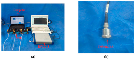
Figure 8.
Test measurement equipment: (a) the Wireless Dynamic Strain Collector; (b) INV9822A accelerometer.
3.4. Test Loading
In this test, a drop hammer was adopted to simulate a rockfall to impact the buried pipeline in the soil-box. Therefore, a drop hammer impact test machine consisting of a support shelf, a drop hammer, two guide rails, and a truss made of four columns and a crossbeam was applied in this test, as shown in Figure 9. The soil-box was placed under the drop hammer impact test machine. The mass of the drop hammer was 339 kg with a maximum impact height of 7.8 m, and the maximum impact energy was 52 kJ. The accelerometer installed on the top of the drop hammer was used to measure the acceleration during the impact. All specimens were buried horizontally in the soil at different depths; then, the soil layers (100 mm thickness per layer) were tamped when the soil was loaded into the soil-box. Finally, the same compactness of the soil was ensured before each impact load test. Meanwhile, the drop hammer was released from the given height and fell down along two rails until impacting directly on the soil, which was located in the mid-span of the pipeline. Preloading was carried out to check whether the test device and measurement system were working properly, and then the formal loading was carried out.
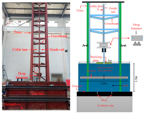
Figure 9.
Schematic diagram of the drop hammer impact test machine.
The impact force (F) in this test could be computed as shown in the equation below.
where m is the mass of the drop hammer, and a denotes the acceleration recorded by the accelerometer during impact.
3.5. Test Results and Discussion
3.5.1. Basic Behavior
The test results of all specimens are presented in Table 2 and Figure 10, which depicts the effect of the wall thickness (T) of the pipeline, the diameter (D) of the pipeline, the buried depth (d) of the pipeline, and the impact height (H) of the drop hammer on the peak strain (ɛmax) at the mid-span of the specimen. It can be seen from Table 2 that, with the same H, D had an obvious influence on ɛmax, while T had a subtle influence on ɛmax. Furthermore, ɛmax decreased with the increase of T, while ɛmax always increased with the increase of D. In addition, we can know that ɛmax decreased rapidly with the increase of d under the same D and T, which indicates that the soil played a good role buffering the impact load. The main reason was that the increases of d absorbed more energy from the impact load via compression in the internal clearance of soil. From Figure 10, it can be seen that the peak longitudinal strain (ɛL) was much larger than the peak transversal strain (ɛT). Furthermore, the maximum deviation of ɛL and ɛT was 33% under the influence of d, and the deviation was approximately equal to 31% under the other three effects. It means that longitudinal bending was the main source of deformation for the specimens under the impact load.
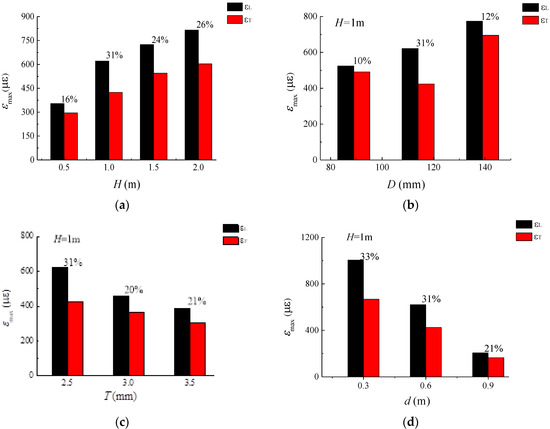
Figure 10.
The effect of the impact height (H), the pipeline diameter (D), the wall thickness (T), and the buried depth (d) on the peak strain (ɛmax): (a) H; (b) D; (c) T; (d) d.
3.5.2. Strain–Time Curves
Taking the A114 × 2.5-d0.6-H1.0 and A114 × 2.5-d0.6-H2.0 samples as examples, the strain–time (ε–t) curves are shown in Figure 11. It can be known from Figure 11a,b that ɛ on the longitude and transverse sections at the mid-span of the specimen increased rapidly and approximately descended to zero after the impact load. Furthermore, compared with ɛT, ɛL was much larger and ε on the upper and lower surfaces of the pipelines showed a symmetrical state. When H was 2 m, ɛL was about 816 με and ɛT was about 603 με. The maximum deviation of ɛL and ɛT was approximately 26%, which indicates that the deformation of the pipeline at the mid-span under the impact load was in the elastic range, and a large elastic deformation was produced in the longitudinal section of the pipeline at mid-span.
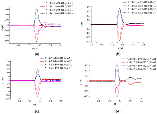
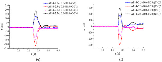
Figure 11.
Strain (ɛ) versus time (t) curves of specimens. (a) A114 × 2.5-d0.6-H1.0, (B–B); (b) A114 × 2.5-d0.6-H2.0, (B–B); (c) A114 × 2.5-d0.6-H1.0, (A–A); (d) A114 × 2.5-d0.6-H2.0, (A–A); (e) A114 × 2.5-d0.6-H1.0, (C–C); (f) A114 × 2.5-d0.6-H2.0, (C–C).
From Figure 11c–f, it can be known that, when H was 2 m, ɛL at positions (A–A)2 and (C–C)2 was 310 με and 300 με, respectively, and ɛT at positions (A–A)1 and (C–C)1 was 200 με and 185 με, respectively. It shows that ɛ at positions (A–A) and (C–C) displayed a symmetrical state. In addition, ɛL at positions (C–C)2 and (C–C)4 was 300 με and 295 με, respectively. It can be seen that ε on the upper and lower surfaces at positions (A–A) and (C–C) also presented a symmetrical state.
It also can be seen from Figure 11 that ɛ increased with the increase of H, and the maximums of ɛ on the longitudinal and transversal sections appeared at the mid-span of the pipeline. This indicates that, with the increase of the distance of the specimen away from the impact area, the strain of the pipeline became small, and the deformation of the pipeline was still in the elastic range even when H was 2 m.
4. Finite Element Analysis (FEA)
To further investigate the strain behavior of buried long pipelines under impact loads, a three-dimensional FEA model was developed to simulate the dynamic response of the pipeline.
4.1. Finite Element Type and Mesh
The FEA model was divided into four parts: the soil, the pipeline, the drop hammer, and the rigid cushion. According to References [41,42], four-node shell elements with reduced integration (S4R) were selected to simulate the pipeline, while eight-node brick solid elements with reduced integration (C3D8R) were used to simulate the soil. In addition, the drop hammer and the rigid cushion were simulated by the four-node three-dimensional rigid elements (R3D4). To ensure the simulation’s effectiveness, a fine mesh was adopted to develop the model by controlling the mesh density, which enhanced the convergence of the FEA result in the algorithm, as shown in Figure 12. In addition, seeds should be scattered on parts by controlling approximate size, then by selecting the element type of mesh parts with a structured mesh method. Based on the global mesh model, the number of elements was 127,300, including 123,252 hexahedral elements (C3D8R and R3D4) and 4048 quadrilateral elements (S4R).
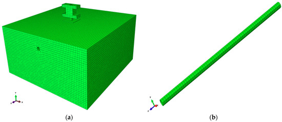
Figure 12.
A three-dimensional finite element analysis (FEA) model: (a) overall mesh of model; (b) local mesh of pipeline.
4.2. Material Model
The Mohr–Coulomb [43,44] model was used for the soil, while the three-fold line model was adopted for the pipeline with consideration of its large deformation, as shown in Figure 13. Meanwhile, the drop hammer and the rigid cushion were regarded as rigid bodies where no deformation occurred during the collision. The stress–strain state of the pipeline can be divided into three stages: elastic stage, elastic–plastic stage, and plastic stage, where ε1, ε2, σ1, and σ2 represent the elastic yield strain, the plastic yield strain, the elastic yield stress, and the plastic yield stress of the pipeline, respectively, and E1 and E2 represent the material modulus of the pipeline at the elastic deformation stage and the stress strengthening stage, respectively. The specific parameters are shown in Table 3 and Table 4.
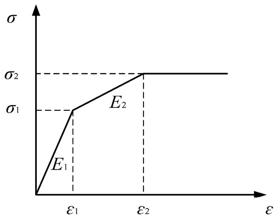
Figure 13.
Schematic diagram of the three-fold line pipeline model.
4.3. The Contact between the Soil and Pipeline
Considering the non-linear contact relationship and the bond-slip effect between the pipeline and soil [45,46], the interaction between interfaces consists of two parts: normal action and tangential action. Tangential action is caused by the relative slip between the pipeline and soil. Normal behavior refers to the distance between the pipeline and soil surface as clearance, and normal pressure can be transferred only when the pipeline is compressed. The hard contact in ABAQUS was adopted to express this normal action, while the tangential action used the Coulomb friction model [47] to transfer the shear stress of the pipeline–soil surface.
4.4. Boundary Conditions and Load Application
According to Reference [48], the upper surface of the soil is free, while all degrees of freedom on the other three surfaces of soil are constrained. During the loading process, the drop hammer was simulated as a free-falling body which had an impact velocity varying with the given impact heights. Because the material model of the soil was the Mohr–Coulomb model that considers the plastic deformation of the soil, the impact collision between the drop hammer and soil was inelastic. In order to enhance the convergence of the predicted result, increments were defined as the automatic type in the analysis step, and the system iterated automatically in the calculation process with a stable incremental size until the calculation results converged.
5. Results and Discussion
5.1. Impact Force
Figure 14 depicts a comparison of impact force–time (F–t) curves on the soil of group A between the depicted results from the FEA and the measured results from the test under different impact heights (H). Furthermore, a comparison of peak impact forces (Fmax) under different values of H among the depicted results from the FEA, measured results from the test (EXP), and theoretical results (THE) deduced from the above theoretical Equation (7) is depicted in Figure 15 and Table 5. It can be found that a generally good agreement was achieved among the results from the FEA, test, and theoretical calculation, which shows that the developed FEA model has a reasonable precision for predicting the impact force on the soil under impact loads and, moreover, the theoretical Equation (7) is capable of calculating the Fmax. Furthermore, the Fmax on the soil was proportional to the impact height. From Table 5, we can also know that the average values and standard deviations of Fmax,FEA/Fmax,EXP and Fmax,THE/Fmax,EXP were 0.954 and 4.61%, and 0.917 and 8.33%, respectively. Nevertheless, there were still some differences among the results, and these may have been induced by the theoretical formula based on the Hertz collision theory, which assumes that collisions are elastic. Furthermore, the influence of the friction force between the drop hammer and guide rail, and the soil compaction in the test were not considered in the FEA model and theoretical formula.
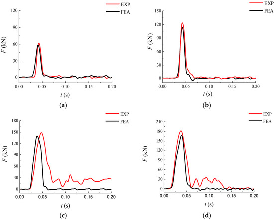
Figure 14.
Comparisons of impact force–time (F–t) curves between the predicted results in FEA and the measured results in the test (EXP) under different impact heights (H): (a) H = 0.5 m; (b) H = 1.0 m; (c) H = 1.5 m; (d) H = 2.0 m.
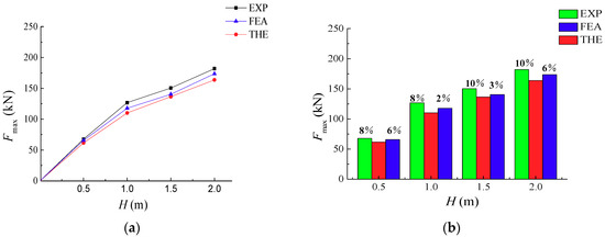
Figure 15.
Comparisons of the peak impact force (Fmax) among the predicted results in FEA, the measured results in the test (EXP), and the theoretical results (THE) under different impact heights (H).
Table 5.
Peak impact force (Fmax) under different impact heights (H). FEA—finite element analysis.
5.2. The Peak Strain
The peak strains of the pipeline at mid-span derived from the FEA were compared with the measured results from the test and theoretical computation, as summarized in Table 6, where the theoretical results were theoretically derived calculated based on the mathematical Equation (21), and the peak strain (εmax, EXP) in the test was calculated based on the peak longitudinal and transverse strains (εL and εT). It can be found from Table 6 that the standard deviations among εmax,EXP and εmax,THE, and εmax,EXP and εmax,FEA were 6.85% and 5.12%, respectively, according to the calculation of the relative deviation between theory and FEA; compared with some references [49,50], the standard deviation of theory and FEA was more accurate. The results show that the peak strain from the FEA results basically matched with the experimental and theoretical results, which verifies the rationality of the mathematical formula and the feasibility of the FEA model. However, some differences still existed. The main reason may be explained by there being some differences in the values of the deformation lag factor and the base coefficient in the theoretical formula, as well as there being some differences in the setting of soil parameters in the FEA.
Table 6.
The peak strains of specimens.
5.3. Strain Distribution
5.3.1. The Influence of Impact Height
Figure 16a shows a comparison of the strain—time (ε–t) curves at the mid-span position (B–B)2 between the depicted results from FEA and the measured results from the experiment (EXP) under different impact heights (H); additionally, a comparison of the peak strains (εmax) at position (B–B)2 among the FEA, EXP, and theoretical (THE) results is also presented in Figure 16b. It can be found from Figure 16 that a generally good agreement was achieved among the FEA, EXP, and THE results, which shows that the developed FEA model has a reasonable precision for predicting the strain of buried pipelines under impact loads. Furthermore, it is shown that H had a significant influence on the mid-span strain, and the εmax increased with the increase of H. When H reached 2 m, the predicted εmax from FEA was 763 με and the position of εmax was as presented in Figure 17d below.
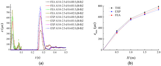
Figure 16.
The influence of impact height (H) on strain: (a) comparisons of strain–time (ε–t) curves between FEA and EXP results under different H; (b) comparisons of the peak strain (εmax) among FEA, EXP, and THE results under different H.
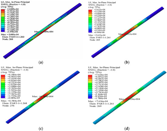
Figure 17.
The influence of impact height (H) on strain distribution: (a) H = 0.5 m; (b) H = 1.0 m; (c) H = 1.5 m; (d) H = 2.0 m.
The influence of impact height (H) on the strain distribution of specimens is depicted in Figure 17. It can be found that the maximum strain area occurred at the mid-span and increased with the increase of H, which matches well with the experimental and theoretical results.
5.3.2. The Influence of Pipeline Diameter and Wall Thickness
Figure 18a,b present the strain–time (ε–t) curves at the mid-span of pipelines considering different values of D (89 mm, 114 mm, and 139 mm) and T (2.5 mm, 3.0 mm, and 3.5 mm), respectively. From Figure 18, it can be seen that the ε–t curves depicted from FEA agreed well with those from EXP, which indicates that the developed FEA model is reasonable to predict the ε–t curves of buried pipelines under impact loads. Furthermore, similar to the above experimental results, the effect of D on ε was more obvious than that of T on ε. Moreover, ɛ increased with the increase of D, while it decreased with the increase of T. The main reason is that the longitudinal stiffness became small with the increase of D, and the pipeline mainly underwent longitudinal bending deformation under the vertical impact load. In addition, a thick wall is helpful to improve the whole rigidity of pipeline. Therefore, a small diameter and a thick wall can improve the ability of the pipeline to resist the impact load.
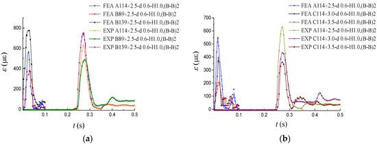
Figure 18.
Comparisons of strain–time (ε–t) curves between FEA and EXP results under different diameter (D) and wall thickness (T): (a) D; (b) T.
Figure 19 plots the influence of diameter (D) and wall thickness (T) on the strain distribution of specimens. The maximum strain region increased with the increase of D, whereas it decreased with the increase of T, which is in good agreement with the experimental results.
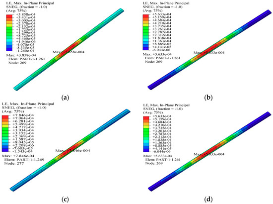
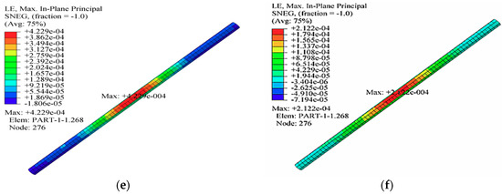
Figure 19.
The influence of diameter (D) and wall thickness (T) on strain distribution: (a) D = 89 mm; (b) D =114 mm; (c) D = 139 mm; (d) T = 2.5 mm; (e) T = 3.0 mm; (f) T = 3.5 mm.
5.3.3. The Influence of Buried Depth
Figure 20a shows a comparison of the strain–time (ɛ–t) curves at the mid-span position (B–B)2 between the predicted results in FEA and the measured results in the experiment (EXP) with various values of buried depth (d); additionally, a comparison of the peak strain (ɛmax) at the position among the FEA, EXP, and theoretical (THE) results is also presented in Figure 20b. It can be found from Figure 20 that a generally good agreement was also achieved among the FEA, EXP, and THE results. Similar to the above experimental results, ɛ reduced with the increase of d. It can also be shown that, when d = 0.25 m, the ɛmax obtained from THE and FEA was more than 1410 με, which indicates that the deformation of the pipeline reached the yield strain. It may be concluded from Figure 20b that a buried depth of the pipeline from 0.5 m to 0.6 m was more reasonable for the pipeline designed in this paper.
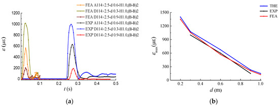
Figure 20.
The influence of burial depth (d) on strain: (a) comparisons of strain–time (ɛ–t) curves between FEA and EXP results under different d; (b) comparisons of the peak strain (ɛmax) among FEA, EXP, and THE results under different d.
The strain distribution of specimens under d in FEA is presented in Figure 21. It can be seen from Figure 21 that ɛ at the mid-span of the specimen with d = 0.9 m (D114 × 2.5-d0.9-H1.0) was much smaller than that with d = 0.6 m (A114 × 2.5-d0.6-H1.0) and d = 0.3 m (D114 × 2.5-d0.3-H1.0), which reflects that the soil plays a buffer role in dispersing the impact load, and indicates that the pipelines cannot be buried shallowly.
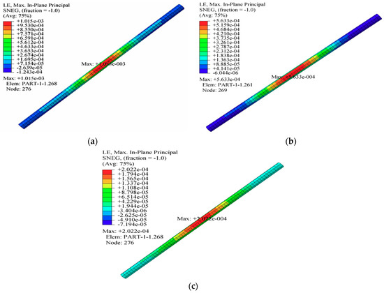
Figure 21.
The influence of burial depth (d) on strain distribution: (a) d = 0.3 m; (b) d = 0.6 m; (c) d = 0.9 m.
6. Conclusions
The strain behavior of a buried long pipeline under an impact load was obtained through comparison among theoretical results (THE), experimental results, and FEA results. The following conclusions can be drawn:
- (1)
- For the buried pipeline under an impact load, a generally good agreement was achieved among the FEA results, the EXP results, and THE results in terms of the peak impact force (Fmax) on soil and the peak strain (ɛmax) on pipelines, which indicates that the mathematical formula based on the mechanical model of a buried pipeline and the finite element models are accurate for the prediction of pipeline response under the impact load.
- (2)
- The peak longitudinal strain (ɛL) was much larger than the peak transversal strain (ɛT); thus, longitudinal bending was the main source of deformation for specimens under the impact load.
- (3)
- Under the same impact height (H) of the drop hammer, the diameter (D) had an obvious influence on ɛmax, while the wall thickness (T) had a subtle influence on ɛmax. Furthermore, ɛmax decreased with the increase of T, while it increased with the increase of D and H, which is similar to the distribution of the high-strain area of the pipeline in the experimental results and FEA results. This means that a small diameter and a thick wall thickness are beneficial for the pipeline to resist the impact load.
- (4)
- The ɛmax decreased rapidly with the increase of the buried depth (d) of the pipeline under the same D and T, which indicates that the pipelines cannot be buried shallowly. According to the extension of THE and FEA results, a buried depth of the pipeline from 0.5 m to 0.6 m was more reasonable for the pipeline designed in this paper.
7. Discussion of Future Work
As an efficient means to transport gaseous and liquid materials, pipelines are widely deployed and play important roles in pipeline network systems. However, the impact load caused by rockfall results in the serious damages of buried pipelines in engineering. In this paper, only the effects of parameters on the strain behaviors of healthy pipelines under impact loads were analyzed through theoretical derivation, experimental research, and finite element analysis (FEA). However, pipelines in service often have pre-existing damages; therefore, a pipeline with pre-existing damages should be considered in future research, and the mechanical properties of damaged buried pipelines under impact loads should be further explored. Benefitting from the recent rapid development of structural health monitoring technology [51,52], many researches demonstrated that piezoceramic materials [53,54] have actuating and sensing ability to detect structural damages. Future research will involve conducting experiments on the damage detection of buried long pipelines with advanced sensing technologies, such as fiber optic sensors [55,56] and piezoceramic transducers [57,58,59], also contributing to the pipeline monitoring. In addition, based on theoretical analysis and numerical simulations, simple design calculations can be proposed.
Author Contributions
All authors discussed and agreed upon the idea, and made scientific contributions. F.D. and G.D. designed the experiments and wrote the paper. F.D., X.B., J.T., and X.X. performed the experiments and analyzed the data.
Funding
The research reported in this paper was partially supported by the National Natural Science Foundation of China (grant number 51778064), the Petro China Innovation Foundation (grant number 2016D-5007-0605), and the Scientific Research Project Foundation of Hubei Provincial Department of Education (grant number 2016CFA022).
Acknowledgments
We acknowledge the help of Xuemeng Bie from the State Key Laboratory of Coastal and Offshore Engineering, Dalian University of Technology.
Conflicts of Interest
The authors declare no conflicts of interest.
References
- Arafah, D.; Madia, M.; Zerbst, U.; Berettaa, S.; Cristea, M. Instability analysis of pressurized pipes with longitudinal surface cracks. Int. J. Press. Vessel. Pip. 2015, 126–127, 48–57. [Google Scholar] [CrossRef]
- Du, G.; Kong, Q.; Zhou, H.; Gu, H. Multiple cracks detection in pipeline using damage index matrix based on piezoceramic transducer-enabled stress wave propagation. Sensors 2017, 17, 1812. [Google Scholar] [CrossRef] [PubMed]
- Li, X.; Bai, Y.; Su, C.; Li, M. Effect of interaction between corrosion defects on failure pressure of thin wall steel pipeline. Int. J. Press. Vessel. Pip. 2016, 138, 8–18. [Google Scholar] [CrossRef]
- Kishawy, H.A.; Gabbar, H.A. Review of pipeline integrity management practices. Int. J. Press. Vessel. Pip. 2010, 87, 373–380. [Google Scholar] [CrossRef]
- Kong, Q.; Robert, R.; Silva, P.; Mo, Y. Cyclic crack monitoring of a reinforced concrete column under simulated pseudo-dynamic loading using piezoceramic-based smart aggregates. Appl. Sci. 2016, 6, 341. [Google Scholar] [CrossRef]
- Hong, X.; Liu, Y.; Lin, X.; Luo, Z.; He, Z. Nonlinear ultrasonic detection method for delamination damage of lined anti-corrosion pipes using PZT transducers. Appl. Sci. 2018, 8, 2240. [Google Scholar] [CrossRef]
- Du, G.; Huo, L.; Kong, Q.; Song, G. Damage detection of pipeline multiple cracks using piezoceramic transducers. J. Vibroeng. 2016, 18, 2828–2838. [Google Scholar] [CrossRef]
- Yun, H.; Kyriakides, S. On the beam and shell modes of buckling of buried pipelines. Soil Dyn. Earthq. Eng. 1990, 9, 179–193. [Google Scholar] [CrossRef]
- Chiou, Y.J.; Chi, S.Y. Beam and shell modes of buckling of buried pipes induced by compressive ground failure. Tech. Counc. Lifeline Earthq. Eng. 1995, 6, 176–187. [Google Scholar]
- Takada, S.; Hassani, N.; Fukuda, K. A new proposal for simplified design of buried steel pipes crossing active faults. Earthq. Eng. Struct. Dyn. 2010, 30, 1243–1257. [Google Scholar] [CrossRef]
- Yan, Y.; Shao, B.; Wang, J.; Yan, X. A study on stress of buried oil and gas pipeline crossing a fault based on thin shell FEM model. Tunn. Undergr. Space Technol. 2018, 81, 472–479. [Google Scholar]
- Chavan, K.S.; Wriggers, P. Consistent coupling of beam and shell models for thermo-elastic analysis. Int. J. Numer. Methods Eng. 2010, 59, 1861–1878. [Google Scholar] [CrossRef]
- Liu, A.; Hu, Y.; Li, X.; Zhao, F.; Takada, S. Damage behavior of large-diameter buried steel pipelines under fault movements. Eng. Mech. 2005, 22, 82–87. [Google Scholar]
- Zhang, J.; Liang, Z.; Han, C.; Zhang, H. Buckling behaviour analysis of a buried steel pipeline in rock stratum impacted by a rockfall. Eng. Fail. Anal. 2015, 58, 281–294. [Google Scholar] [CrossRef]
- Liu, M.; Min, Y. Modeling the behavior of natural gas pipeline impacted by falling objects. Eng. Fail. Anal. 2014, 42, 45–59. [Google Scholar] [CrossRef]
- Deng, X.; Xue, S.; Tong, X. Numerical simulation on response of buried pipeline induced by rock-fall transverse impaction. J. China Univ. Pet. 2009, 33, 111–115. [Google Scholar]
- Chen, J.; Wang, Q.; Chen, Y.; Li, J. Amending calculation on impact force of boulders in debris flow based on Hertz theory. J. Harbin Inst. Technol. 2017, 49, 124–129. [Google Scholar]
- Ruta, P.; Szydło, A. Drop-weight test based identification of elastic half-space model parameters. J. Sound Vib. 2005, 282, 411–427. [Google Scholar] [CrossRef]
- Zhao, G.; Li, S.; Xiong, Z.; Gao, W.; Han, Q. A statistical model of elastic-plastic contact between rough surfaces. Trans. Can. Soc. Mech. Eng. 2019, 43, 38–46. [Google Scholar] [CrossRef]
- Gutzwiller, M.C. The impact of a rigid circular cylinder on an elastic solid. Philos. Trans. R. Soc. B Biol. Sci. 1962, 255, 153–191. [Google Scholar] [CrossRef]
- Qi, S.; Zhou, C.; Liu, S.; Song, X. Study on Impact Force of Landfall and Rockfall. Appl. Mech. Mater. 2013, 256–259, 81–85. [Google Scholar] [CrossRef]
- Ye, S.; Chen, H.; Tang, H. The calculation method for the impact force of the rockfall. China Railw. Sci. 2010, 31, 56–62. [Google Scholar]
- Marston, A.; Anderson, A.O. The Theory of Loads on Pipes in Ditch and Tests of Cement and Clay Drain Tile and Sewer Pipe; Iowa State College of Agriculture and Mechanic Arts: Iowa City, IA, USA, 1913; pp. 45–196. [Google Scholar]
- Kang, J.; Parker, F.; Yoo, C. Soil-structure interaction and imperfect trench installations for deeply buried concrete pipes. J. Geotech. Geoenviron. Eng. 2007, 133, 277–285. [Google Scholar] [CrossRef]
- Hindy, A.; Novak, M. Earthquake response of underground pipelines. Earthq. Eng. Struct. Dyn. 1979, 7, 451–476. [Google Scholar] [CrossRef]
- Zheng, J.; Zhao, J.; Chen, B. Vertical earth pressure on culverts under high embankments. Chin. J. Geotech. Eng. 2009, 31, 1009–1013. [Google Scholar]
- Ning, B.K.; Fan, H.; Gong, L.; Liu, G. Study on vertical earth pressure of slab culvert under high embankment. Appl. Mech. Mater. 2013, 256–259, 1898–1902. [Google Scholar] [CrossRef]
- Zhou, S.; Sun, X.; Peng, J.; Lv, J. A study on the earth pressure of top culvert of high embankment. Appl. Mech. Mater. 2012, 178–181, 1104–1111. [Google Scholar] [CrossRef]
- Yun, L.; Kang, L. Reliability analysis of high pressure buried pipeline under landslide. Appl. Mech. Mater. 2014, 501–504, 1081–1086. [Google Scholar] [CrossRef]
- Jing, H.; Deng, Q.; Hao, J.; Han, B.; Li, L. Analysis and numerical simulation on dynamic response of buried pipeline caused by rock fall impaction. Proc. Bienn. Int. Pipeline Conf. 2012, 2, 303–311. [Google Scholar]
- Zhang, H.; Zhang, J.; Liu, S. Mechanical properties of the buried pipeline under impact load caused by adjacent heavy tamping construction. J. Fail. Anal. Prev. 2016, 16, 647–654. [Google Scholar] [CrossRef]
- The American Society of Civil Engineers. Guidelines for the Design of Buried Steel Pipeline; The American Society of Civil Engineers: Reston, VA, USA, 2005. [Google Scholar]
- Wang, G.; Qu, S.; Hou, X.; Zhu, F.; Zhang, J. Preliminary study on vertical subsoil participating mass. Adv. Mater. Res. 2011, 199–200, 1429–1434. [Google Scholar] [CrossRef]
- Terzaghi, K.; Peck, R.B.; Mesri, G. Soil mechanics in engineering practice. In A Wiley-Interscience Publication, 3rd ed.; John Wiley and Sons Inc.: Hoboken, NJ, USA, 1996. [Google Scholar]
- GB 50253-2003 Code for Design of Oil Pipeline Engineering; Planning Press: Beijing, China, 2003.
- Tian, Y.; Liu, H.; Jiang, X.; Yu, R. Analysis of stress and deformation of a positive buried pipe using the improved Spangler model. Soils Found. 2015, 55, 485–492. [Google Scholar] [CrossRef]
- Xiao, J.; Zhang, X.; Chen, J.; Li, Z. Study on 3d Flexible Pipe FEM Analysis by Spangler Theory. Adv. Mater. Res. 2014, 850–851, 821–824. [Google Scholar] [CrossRef]
- She, Y. Study on the effect of vibration loads induced by bridge pile foundation construction on adjacent buried pipeline. Appl. Mech. Mater. 2013, 353–356, 191–197. [Google Scholar] [CrossRef]
- Prisco, C.D.; Andrea, G. Mechanical behavior of geo-encased sand columns: Small scale experimental tests and numerical modeling. Geomech. Geoengin. 2011, 6, 251–263. [Google Scholar] [CrossRef]
- Wijewickreme, D.; Karimian, H.; Honegger, D. Response of buried steel pipelines subjected to relative axial soil movement. Can. Geotech. J. 2009, 46, 735–752. [Google Scholar] [CrossRef]
- Magda, W. Wave-induced uplift force acting on a submarine buried pipeline: Finite element formulation and verification of computations. Comput. Geotech. 1996, 19, 47–73. [Google Scholar] [CrossRef]
- Li, X.; Sun, J.; Li, T. The analysis and comparison of all kinds of buried pipeline model based on seismic effect. Engineering 2016, 8, 365–370. [Google Scholar] [CrossRef][Green Version]
- Robert, D.J. A modified Mohr-Coulomb model to simulate the behavior of pipelines in unsaturated soils. Comput. Geotech. 2017, 91, 146–160. [Google Scholar] [CrossRef]
- Hosseinpour, I.; Mirmoradi, S.H.; Barari, A.; Omidvar, M. Numerical evaluation of sample size effect on the stress-strain behavior of geotextile-reinforced sand. J. Zhe Jiang Univ. Sci. A 2010, 11, 555–562. [Google Scholar] [CrossRef]
- Zeng, X.; Dong, F.; Xie, X.; Du, G. A new analytical method of strain and deformation of pipeline under fault movement. Int. J. Press. Vessel. Pip. 2019, 172, 199–211. [Google Scholar] [CrossRef]
- Daiyan, N.; Kenny, S.; Phillips, R.; Popescu, R. Investigating pipeline-soil interaction under axial-lateral relative movements in sand. Can. Geotech. J. 2011, 48, 1683–1695. [Google Scholar] [CrossRef]
- Roy, K.; Hawlader, B.; Kenny, S.; Moore, I. Finite element modeling of lateral pipeline-soil interactions in dense sand. Can. Geotech. J. 2015, 53, 490–504. [Google Scholar] [CrossRef]
- Zhang, J.; Liang, Z.; Feng, D.; Zhang, C.; Xia, C.; Tu, Y. Response of the buried steel pipeline caused by perilous rock impact: Parametric study. J. Loss Prev. Process Ind. 2016, 43, 385–396. [Google Scholar] [CrossRef]
- Xu, T.; Yao, A.; Jiang, H.; Li, Y.; Zeng, X. Dynamic response of buried gas pipeline under excavator loading: Experimental/numerical study. Eng. Fail. Anal. 2018, 89, 57–73. [Google Scholar] [CrossRef]
- Yao, A.; Xu, T.; Zeng, X.; Jiang, H. Numerical analyses of the stress and limiting load for buried gas pipelines under excavation machine impact. J. Pipeline Syst. Eng. Pract. 2015, 6, A4014003. [Google Scholar] [CrossRef]
- Kong, Q.; Shuang, H.; Ji, Q.; Mo, Y.; Song, G. Very early age concrete hydration characterization monitoring using piezoceramic based smart aggregates. Smart Mater. Struct. 2013, 22, 085025. [Google Scholar] [CrossRef]
- Jia, Z.; Ren, L.; Li, H.; Ho, S.; Song, G. Experimental study of pipeline leak detection based on hoop strain measurement. Struct. Control Health Monit. 2015, 22, 799–812. [Google Scholar] [CrossRef]
- Zhu, J.; Ren, L.; Ho, S.; Jia, Z.; Song, G. Gas pipeline leakage detection based on PZT sensors. Smart Mater. Struct. 2017, 26, 025022. [Google Scholar] [CrossRef]
- Zhang, G.; Zhu, J.; Song, Y.; Peng, C.; Song, G. A time reversal based pipeline leakage localization method with the adjustable resolution. IEEE Access 2018, 6, 26993–27000. [Google Scholar] [CrossRef]
- Inaudi, D.; Glisic, B. Long-Range pipeline monitoring by distributed fiber optic sensing. J. Press. Vessel Technol. 2010, 132, 011701. [Google Scholar] [CrossRef]
- Jia, Z.; Ren, L.; Li, H.; Sun, W. Pipeline leak localization based on FBG hoop strain sensors combined with BP neural network. Appl. Sci. 2018, 8, 146. [Google Scholar] [CrossRef]
- Sethi, V.; Song, G. Optimal vibration control of a model frame structure using piezoceramic sensors and actuators. JVC J. Vib. Control 2005, 11, 671–684. [Google Scholar] [CrossRef]
- Du, G.; Kong, Q.; Wu, F.; Ruan, J.; Song, G. An experimental feasibility study of pipeline corrosion pit detection using a piezoceramic time reversal mirror. Smart Mater. Struct. 2016, 25, 037002. [Google Scholar] [CrossRef]
- Wang, F.; Huo, L.; Song, G. A piezoelectric active sensing method for quantitative monitoring of bolt loosening using energy dissipation caused by tangential damping based on the fractal contact theory. Smart Mater. Struct. 2017, 27, 015023. [Google Scholar] [CrossRef]
© 2019 by the authors. Licensee MDPI, Basel, Switzerland. This article is an open access article distributed under the terms and conditions of the Creative Commons Attribution (CC BY) license (http://creativecommons.org/licenses/by/4.0/).