Autonomous Load Regulation Based Energy Balanced Routing in Rechargeable Wireless Sensor Networks

Abstract

Recent progress in wireless charging technologies has greatly promoted the development of rechargeable wireless sensor networks (RWSN). The network lifetime of RWSN can be commonly extended through routing strategy and wireless charging technology. However, the node accepts the relay request of its neighbor unconditionally, and it cannot remove its overload on its own in a timely manner in traditional routing strategies. The energy balancing efficiency of the network may be limited by this passive mechanism, which poses a great challenge to obtaining optimal joint efficiency of routing and charging strategies. In this paper, we propose an autonomous load regulation mechanism-based energy balanced routing algorithm (ALRMR) for RWSN. In addition to an efficient framework of joint wireless energy transfer and multi-hop routing where the routing strategy is adapted to the charging scheme, an innovative load regulation mechanism is proposed. Under this mechanism, each node can actively adjust its own load by controlling its relay radius. The simulation demonstrates the advantages of our algorithm for energy balance efficiency and improving the network lifetime through the charging scheme and the innovative mechanism.

1. Introduction

Wireless sensor networks provide an efficient and inexpensive communication solution for many applications in the Internet of Things. However, the network lifetime is limited by the small-capacity batteries of sensors [1]. Though some methods to prolong the lifetime have been put forward, including energy harvesting [2] and node reclamation [3], it is still difficult to maintain a steady energy supply due to the application environments [4]. Another reliable method is urgently needed to guarantee the longevity of sensors.

Wireless charging technology provides relatively reliable energy supply for wireless sensor networks (WSN). Kurs [5] demonstrated the feasibility of wireless energy transfer. Sensors can obtain energy within a certain distance by coupling resonances. The corresponding wireless charging device can be placed on the mobile vehicle to replenish energy for nodes, which can extend the network lifetime stably [6].

Based on the wireless energy transfer, the network lifetime can still be extended by joint routing algorithms [7,8,9]. Each node selects its next hop according to link states and most data packets flow to the sink via the nodes with a better energy state when a mobile charger vehicle (MCV) charges for the nodes with low energy, which has a great influence on the lifetime of the WSN.

However, the node accepts the relay request of its neighbor unconditionally in traditional multi-hop routing strategy and cannot remove its overload by itself in a timely manner [10]. The load balancing efficiency of the network is limited by this passive mechanism. Moreover, the energy balance efficiency of an MCV may be reduced due to the energy replenishment of a few high-load nodes over a long time period, which poses a great challenge to obtaining optimal joint efficiency of routing and charging strategies.

Based on these observations, we propose an autonomous load regulation mechanism-based energy balanced routing algorithm (ALRMR) for rechargeable wireless sensor networks (RWSN) in this paper. The ALRMR connects the wireless energy transfer with multi-hop routing, where the routing is adapted to the charging scheme. Furthermore, an autonomous load regulation mechanism is proposed, where every node can actively adjust its own load by controlling its relay radius. The simulation demonstrates the advantages of our algorithm for energy balance efficiency and improving the lifetime through the charging scheme and autonomous load regulation mechanism.

The main contribution of this paper is the proposal of the ALRMR. Moreover, its practicability is proven by simulation. The ALRMR improves energy balance efficiency and prolongs network lifetime through reasonable energy allocation and an autonomous load regulation mechanism.

The rest of this paper is organized as follows: Section 2 introduces recent developments for charging and routing algorithms in WSN. Section 3 introduces the system model. Section 4 and Section 5 describe our charging scheme and routing algorithm, respectively, in detail. Section 6 provides the simulation results and Section 7 presents a summary and future works.

2. Related Work

Many scientists have devoted efforts to optimize charging schemes that can prolong the lifetime of WSN. A number of studies have focused on the adjustments of the traverse route of a single MCV to improve charging efficiency and extend network lifetime. Erol-Kantarci [11] proposed an optimization model to select the minimum number of landmarks according to the locations and energy replenishment requirements of the sensors. Xie [12] developed a near-optimal solution by a piecewise linear approximation technique to optimize the traverse route. An MCV can only charge a single node at a time in the algorithm mentioned above. For higher charging efficiency and less travel distance, Xie [13] used Reformulation-Linearization Technique (RLT) to optimize the charging algorithm with multi-node charging technology. Wu [14] used the algorithm Multi-node Renewable based on Charging Range (MRCR) to obtain a shortest length in every round to improve charging efficiency. However, the algorithms above ignored the importance of reasonable power allocation for multiple nodes. Due to the high transmission loss rate of wireless energy, an MCV should allocate power for each node in the same cell according to their charging efficiencies and energy states reasonably. Our algorithm uses an efficient power allocation scheme to charge for low energy nodes in a timely manner, and can thus extend the network lifetime.

Another effective way to extend the lifetime of WSN is by optimizing routing algorithms. Numerous multi-hop routing algorithms balance load through next-hop selection. Ehsan [15] used the principles of fuzzy ant colony optimization routing (FACOR) to develop a suitable problem solution. Tang [16] proposed the gravitation model to balance energy by ‘space gravitation’, considering the spatial relationship of nodes and ‘time gravitation’, which takes into account the waiting time of data packets. Cai [17] proposed a dynamic energy balance max flow routing algorithm to maximize the load flow within the network lifetime and balance energy consumption to prolong the network lifetime. Ding [18] proposed a solution to sufficiently maintain energy efficiency and avoid congestion for energy-unlimited WSN. Zou [19] proposed an improved ant colony algorithm that can be used to construct the sensor node transfer function and pheromone update rule; it can also adaptively choose a data route by adopting the advantages of the dynamic state of the network. However, current energy-efficient routing strategies and charging technologies are relatively mature. The effect of extending the network lifetime is limited by simply relying on the optimization of a routing strategy. Our algorithm connects wireless charging technology with a routing strategy effectively, where the nodes with low energy can obtain energy replenishment in a timely manner. Thus, the network lifetime can be extended greatly.

Inspired by the effects of extending network lifetime, some works have connected the multi-hop routing strategy with charging technology. Aslam [20] attempted an approach based on the shortest path algorithm and grid clustering to save and renew power in a way that minimizes energy consumption and prolongs the overall network lifetime of WSN. Tang [21] proposed an optimization algorithm from the aspects of both charging and routing processes. In [22], a joint energy supply and routing path selection algorithm was proposed to extend the network lifetime based on an initiative power supply. However, the node accepts the relay request of its neighbor unconditionally in the routing algorithms above and cannot remove its overload by itself in a timely manner. The load balancing efficiency of the network is limited by this passive mechanism. Furthermore, the energy balance efficiency of an MCV may be reduced due to the energy replenishment of a few high-load nodes over a long time period. Therefore, an autonomous load regulation mechanism is proposed in this paper, where every node can actively adjust its own load by controlling its relay radius. The lifetime can be extended through this autonomous load regulation mechanism.

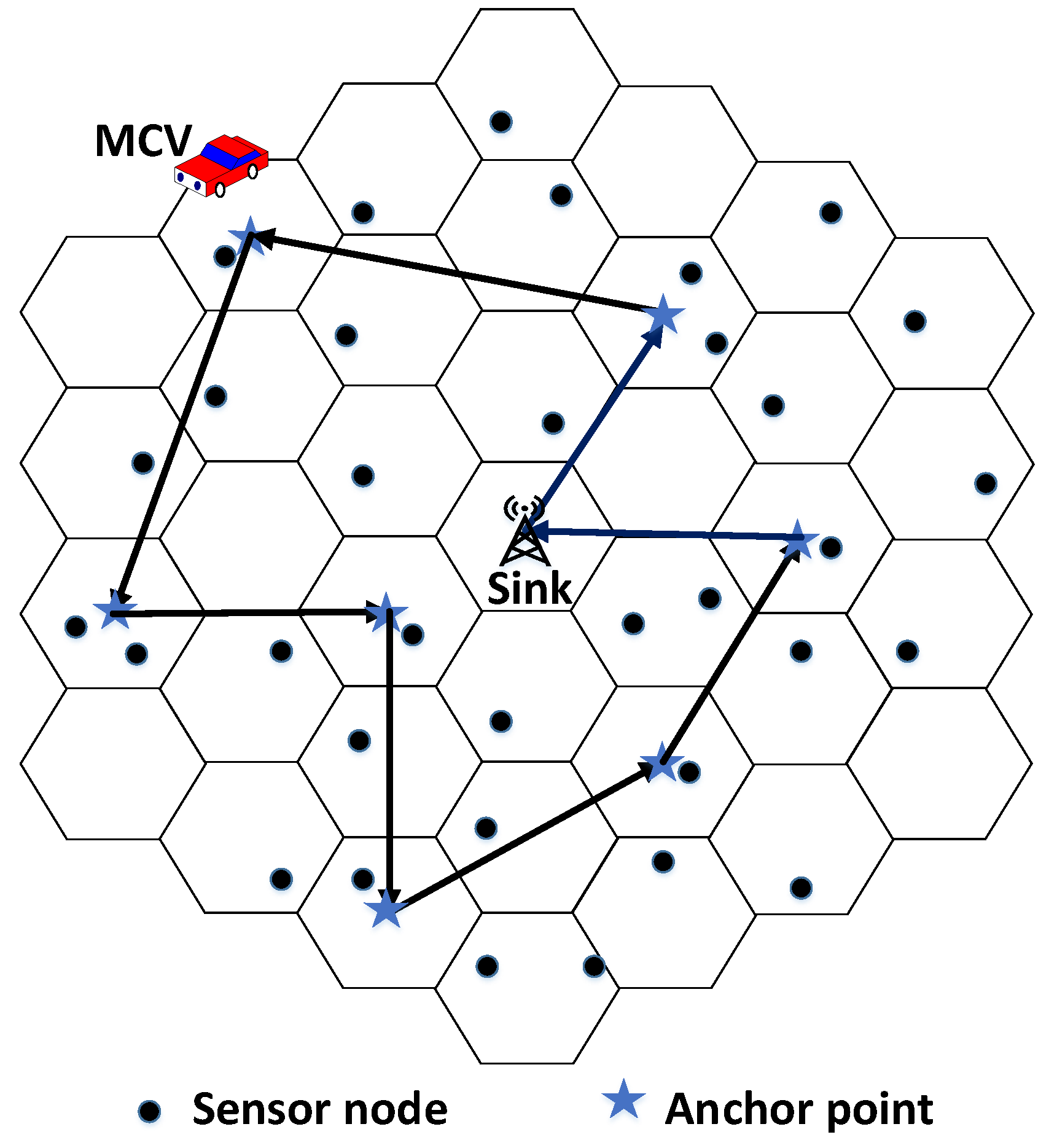
3. System Model

To recharge the battery and gather data from nodes, an MCV is employed. Ideally, we aim to solve a problem where the MCV can stop anywhere within the two-dimensional plane and charge sensor nodes wirelessly. However, an infinite number of possible locations can lead to an infinite size of search space. We simplify this problem by introducing a logical cellular structure, as shown in Figure 1. The two-dimensional plane is partitioned with hexagonal cells with a side length of $R$. The cells that the MCV need to charge for are determined by locations and energy states of nodes. The MCV uses its center as an anchor point and only works when it sojourns at these points. The MCV travels from the base station to each anchor point at a speed of $S$ along the direction of the arrows in order to charge the nodes. Due to the low power reception efficiency caused by the long distance, we assume that the node can be charged only if the MCV sojourns at its cell. It returns to the base station to supplement its own energy when all charging cells have been charged.

The network is defined by the directed graph G (C,V,E). The $c_m\in C$ represents a cell and $m$ is the serial number of a cell. Each vertex $v_i\in V$ represents a sensor node and each edge $l_{ij}\in E$ represents a directed communication link between node $v_i$ and its forward node $v_j$, where $i$ and $j$ are serial numbers of nodes. The communication link can only exist if $v_j$ is within the transmission range of $v_i$. There are $N$ randomly distributed fixed sensor nodes in a two-dimensional plane. Every sensor has a battery capacity of $E_o$ and is fully charged initially. Each of them, with a maximum communication distance of $D$, has the corresponding energy consumption when the node collects, sends, and receives data. The highest energy consumption of the node is derived from the process described above, so the remaining energy consumption is ignored in this paper [23]. All packets are of the same constant size.

3.1. Energy Transfer Model

Each node in the same charging cell can be charged by the MCV simultaneously. Taking node $v_i$ as an example, its energy transfer efficiency ${\eta }_i$ is calculated as follows [24]:

$${\eta }_i=\frac{G_S{G}_R}{L_P}{\left(\frac{\lambda }{4\pi (d_{i,c_m}+\beta )}\right)}^2,i\in c_m$$

(1)

where $G_S$ is the source antenna gain and $G_R$ is the receiving antenna gain. $\lambda$ is the wavelength and $L_P$ is polarization loss. $\beta$ is a parameter to adjust the Friis free space equation for short-distance transmission. $d_{i,c_m}$ is the distance between node $v_i$ and its cell center. The efficiency decreases dramatically with the increase of distance.

3.2. Traffic Load Model

The load of each node is quantified by the traffic it relays. It is assumed that every node generates ${\lambda }_i^s$ data packets per round and the load of a node can be calculated by Formula (2).

$$l_i={\lambda }_i^s+{\displaystyle \sum _{j\in BF(i)}{l}_j}$$

(2)

where $l_i$ and $l_j$ are the traffic loads of node $v_i$ and node $v_j$, respectively. $BF(i)$ is the subset of node $v_i$ and the nodes in $BF(i)$ send the data they need upload to node $v_i$ for relay. $l_i$ reflects the load of the node through the network traffic distribution, which refers specifically to the number of data packets needed to be uploaded in each round. A data packet is the traffic corresponding to the unit load. The nodes in the areas where traffic converges are heavily loaded.

4. Energy Replenishment Strategy

The MCV only charges some of the whole cells per round. The rationality of the selection of which cells are charged determines the energy replenishment efficiency. This section describes how to determine the charging cells and energy replenishment scheme based on the energy states of nodes.

4.1. Charging Cells Selection

The energy states of nodes change over time in WSN. The nodes with low residual energy and high energy consumption should have a higher priority of replenishment for the integrity of the network. In the meantime, the charging efficiency of the MCV is related to the number of charging cells. A large number of charging cells allows more nodes to gain energy replenishment in time, but this will the increase the moving time of the MCV and reduce the charging efficiency. Based on the observations above, we selected the charging cells as follows.

The MCV calculates the charging efficiency of cells based on the state information of all nodes at the beginning of each round. Taking cell $c_m$ as an example, its charging efficiency is calculated as follows:

$$c{e}_{c_m}=\underset{i\in c_m}{\min }(\frac{e_i}{E_i})$$

(3)

where $E_i$ and $e_i$ are the residual energy and the energy consumption of node $v_i$ in the previous round, respectively. It is assumed that the energy consumption is zero and the residual energy is $E_o$ for all nodes in the first round. The MCV can reach higher charging efficiency in the cells where the nodes with low residual energy and high energy consumption are located.

Then, the MCV sorts the cells in a decreasing order according to their charging efficiencies and records the sorted list by $PAS$. $PAS(m)$ denotes the ith element in the list of $PAS$, specifically referring to the cell with the ith largest charging efficiency. Thus, $PAS$ is a sorted list of cells containing charging efficiency information. The MCV, starting from the first element, extracts cells to charge them one by one sequentially according to the $PAS$ and controls the number of charging cells based on the energy dispersion. The energy dispersion is calculated as follows:

$$\alpha =\frac{1}{ace}\sqrt{\frac{1}{\left|AC\right|}{\displaystyle \sum _{c_m\in AC}(c{e}_{c_m}-ace}{)}^2}$$

(4)

where $AC$ is the set of cells where all nodes are located and $\left|AC\right|$ is the number of elements in set $AC$. $ace$ is the average charging efficiency of all cells in $AC$. $\alpha$ is the energy dispersion of cells in set $AC$; a higher $\alpha$ means that the energy states of cells have great differences. Using energy dispersion, the charging cells can be determined as follows:

$$CV=\{PAS(m)|m\in [1,n],n=\lfloor (1-\alpha )\left|AC\right|\rfloor \}$$

(5)

where $CV$ contains all charging cells in one round. Based on the mechanism above, the MCV charges more cells when the network energy distribution is uniform in order to maintain the overall energy level of the network. In addition, it reduces the number of charging cells when the energy dispersion is large in order to enhance the energy replenishment for low energy nodes.

4.2. Charging Time and Charging Power Allocation

The MCV replenishes the energy of nodes with the objective of maximizing the network lifetime. With the given sequence of charging cells, we can formulate the sojourn time and charging power allocation problem into the following optimization problem:

$$\underset{(P_i,t_{c_m})}{max}{\displaystyle \sum _{m\in CV}{\displaystyle \sum _{i\in c_m}\log (1+\frac{{\eta }_i{P}_i{t}_{c_m}}{E_i})}}$$

(6)

subject to

$${\displaystyle \sum _{i\in c_m}{P}_i\le P}$$

(7)

$${\eta }_i{P}_i{t}_{c_m}+E_i\le E_o,i\in c_m$$

(8)

$$t_{c_m}/c{e}_{c_m}=t_{c_k}/c{e}_{c_k}\forall m,k\in CV$$

(9)

$${\displaystyle \sum _{c_m\in CV}{t}_{c_m}}\le T-t_{tsp}$$

(10)

where $P_i$ is the charging power for node $v_i$. $t_{c_m}$ and $t_{c_k}$ are the charging times for cell $c_m$ and cell $c_k$, respectively. $T$ is the time of one round. $t_{tsp}$ is the minimum time that it takes for the MCV to visit all cells in $CV$, and we use the TSP algorithm [25] to find the shortest distance among their centers.

The charging power constraint (7) states that the sum of charging power allocated for all nodes in the same cell cannot exceed the maximum power of the MCV. The battery capacity constraint (8) states that the sum of the supplementary energy and residual energy for any node in a round cannot exceed the battery capacity of the sensors. These constraints ensure that the MCV can reasonably use its own charging capability without any energy wasting behavior.

The energy balance constraint (9) states that the charging time allocated for each cell is positively correlated with its own charging efficiency, and the cell with the high charging efficiency can get more charging time. The charging time constraint (10) states that charging time is limited by the mobile time and round time.

The optimization problem calculates the charging effects of different schemes through the objective function (6). According to the optimal solution, the MCV allocates charging time for each cell and charging power for each node in the same cell based on multi-point charging technology. Nodes with low energy and high energy consumption will get higher energy supplement and the balance of the network energy distribution can be ensured.

5. Routing Algorithm Based on Autonomous Load Regulation Mechanism

The node accepts the relay request of its neighbor unconditionally in traditional multi-hop routing and cannot remove its overload by itself in a timely manner. The load balance efficiency of the network is limited by this passive mechanism. In this section, the autonomous load regulation mechanism is formulated based on data relay radius control and the corresponding routing algorithm combined with the charging scheme.

5.1. Autonomous Load Regulation Mechanism Based on Data Relay Radius Control

In order to enable each node to accurately analyze its relative load level and control its own load in a timely manner, we proposed an autonomous load regulation mechanism based on data relay radius control. Taking node $v_j$ as an example, the relationship between the data relay radius and the relay range is as follows:

$$RR(j)=\left\{i\right|d_{js}<d_{is},d_{ij}<r_j,i\in V\}$$

(11)

where $RR(j)$ is the relay range of node $v_j$, while $d_{is}$ and $d_{js}$ are the distances from node $v_i$ and node $v_j$ to the sink, respectively. $d_{ij}$ is the distance between node $v_i$ and node $v_j$. $r_j$ is the data relay radius of node $v_j$ and node $v_j$ only accepts relay requests of the nodes in its relay range.

Based on the relationship above, the autonomous load regulation mechanism based on data relay radius control is described in Algorithm 1.

Algorithm 1: Autonomous load regulation mechanism based on data relay radius control.

for all $v_j\in V$  if $l_j-\overline{l_j}>\gamma ·\overline{l_j}$ and $r_j>0$ then $r_j--$;  else if $\overline{l_j}-l_j>\gamma ·\overline{l_j}$ and $r_j<R$ then $r_j++$;  else do nothing  end if end for

where $\overline{l_j}$ is the average load of node $v_j$ and its neighbors, $\gamma$ is the load regulation accuracy, and $\gamma ·\overline{l_j}$ is the threshold of load difference. If $l_j$ is more than $\gamma ·\overline{l_j}$ compared with $\overline{l_j}$, node $v_j$ is seriously overloaded and it should reduce its data relay radius in order to decrease its relay range and load. If $l_j$ is less than $\gamma ·\overline{l_j}$ compared with $\overline{l_j}$, node $v_j$ has a light load and it should increase its data relay radius and relay range in order to share load for its neighbors. If the difference between $l_j$ and $\overline{l_j}$ is less than $\gamma ·\overline{l_j}$, node $v_j$ is in the appropriate load state, and its relay radius does not need to be adjusted.

5.2. Link State Evaluation

The state of communication link is closely related to the energy state of nodes in WSN. Combined with the charging scheme, we evaluated the link state based on the energy state of nodes and energy efficiency. Firstly, the autonomous load regulation mechanism is used to set up the available forward neighbor sets for each node. Taking node $v_i$ as an example, its available forward neighbor set is as follows:

$$AFN(i)=\left\{j\right|d_{js}<d_{is},d_{ij}<r_j,j\in V\}$$

(12)

where $AFN(i)$ is the available forward neighbor set of node $v_i$. Considering the relay radius of each forward neighbor, the set records all available next-hop options of node $v_i$.

Then we evaluated the energy state of the potential next hop. Energy storage level is a key factor in analyzing the energy state due to the limited battery capacity. Using residual energy and traffic load, the energy storage level can be calculated as follows:

$$ES{L}_{ij}=\frac{E_j+E_j^c}{l_i+l_j}j\in AFN(i)$$

(13)

where $ES{L}_{ij}$ is the energy storage level of node $v_j$ if it is the next hop of node $v_i$, while $E_j^c$ is the supplementary energy of node $v_j$ in a round based on the charging scheme. This indicator is used to represent the energy surplus for the current load. Furthermore, the available next hop with a high energy and low load has the higher relay priority in order to balance the energy of its neighbors.

In addition to the energy storage level, the energy efficiency of the source node is also important in evaluating the link state. The node should cause the packets to flow along the direction from the source node to the sink in order to avoid energy waste when uploading data. Taking node $v_j$ as an example, the energy efficiency can be calculated as follows:

$$E{E}_{ij}=\frac{e_{is}-e_{js}}{e_{ij}}j\in AFN(i)$$

(14)

where $e_{is}$ and $e_{js}$ are the energy consumption of sending a data packet directly to sink by node $v_i$ and by node $v_j$, respectively, and $e_{ij}$ is the energy consumption of sending a packet to node $v_j$ by node $v_i$. The difference between $e_{is}$ and $e_{js}$ represents the active energy consumption of sending a packet and $e_{ij}$ represents the actual energy consumption of sending a packet. A greater $E{E}_{ij}$ indicates higher energy efficiency.

The energy storage level considers the energy states of available next hops, which can enhance the evasion ability of data packets to avoid low energy nodes when they flow to the sink. Energy efficiency can establish efficient routing and avoid energy waste. Combining these two factors, the link state can be evaluated as follows:

$$L{S}_{ij}=\log {(1+ES{L}_{ij})}^{E{E}_{ij}}j\in AFN(i)$$

(15)

where $L{S}_{ij}$ is the link state of node $v_i$ and node $v_j$. In order to balance energy, this indicator helps each node choose the optimal next hop by considering residual energy, charging scheme, traffic load, and energy consumption. Data packets can bypass the overloaded node to reach the sink while considering energy efficiency by the link state.

5.3. Routing Setup and Update

The states of nodes change with time and the network needs to update the routing scheme in a timely manner in order to optimize the network performance. The sink broadcasts the charging scheme, data relay radius, and relative state parameters of nodes in the previous round at the beginning of each round. Each node calculates the link state of its available forward neighbors and determines the optimal next hop according to the broadcast information. The specific process is given in Algorithm 2.

Algorithm 2. Routing setup and update strategy of the autonomous load regulation mechanism-based energy balanced routing algorithm (ALRMR).

Inputs:V, state information of all nodes; Outputs: Network routing $V.next$; for all vi ∈ V  $FN(i)=\left\{j\right|d_{js}<d_{is},d_{ij}<R,j\in V\}$;  $AFN(i)=\left\{j\right|d_{js}<d_{is},d_{ij}<r_j,j\in V\}$;  if $AFN(i)\ne \varphi$ then $v_i.next\leftarrow \arg {\max }_{v_{j\in AFN(i)}}\left\{L{S}_{ij}\right\}$;  else $v_i.next\leftarrow \arg {\max }_{v_{j\in FN(i)}}\left\{E_j\right\}$  end if end for $V.next=\{v_i.next|\forall v_i\in V\}$

Each node establishes its available forward neighbor set and chooses the next hop with the optimal link state. Some nodes may have no available forward neighbors, depending on the routing setup. This is because all forward neighbor of these nodes have a short data relay radius due to overload, so the node will choose the forward neighbor with the highest energy as the next hop in order to ensure data upload. Data packets from these nodes are tagged and any node will relay them unconditionally. Each node updates its status parameters at the end of the round and uploads the information to the sink in order to provide data support for the routing update and charging scheme in the next round.

The operation principle of our routing strategy can be described by Figure 2, where the shadow area is the relay range of node B according to Formula (11) and the squares near the nodes represent their loads. It is assumed that nodes F and G choose node B as their next hops, according to the link state. Thus, node B has a higher energy consumption and needs to reduce its load appropriately. However, if node B cannot remove its load automatically, it can only wait for its subnodes (nodes F and G) to change their next hops due to the significant decrease of node B’s residual energy, which greatly reduces the energy balance efficiency. Using the autonomous load regulation mechanism, node B can become aware of its heavy load state and remove some load by decreasing its data relay radius in a timely fashion. Then node G has to immediately change its next hop, which can balance the load of nodes and the network energy distribution efficiently.

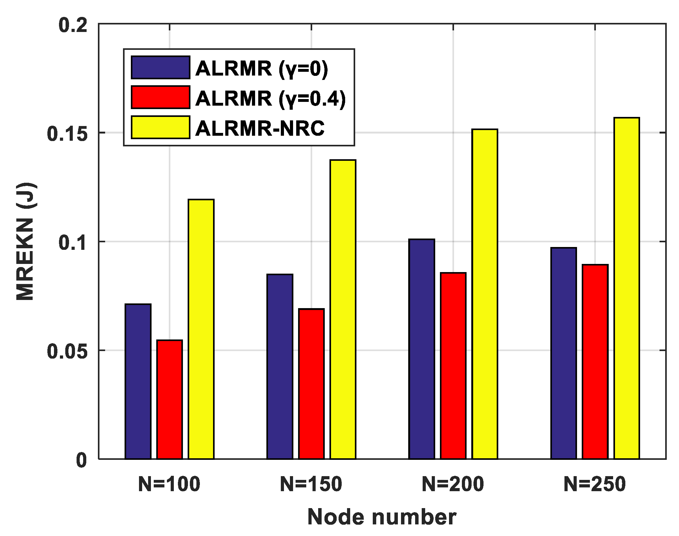
6. Performance Evaluation

In order to evaluate the performance of the algorithm, we used MATLAB to simulate the algorithm. The simulation parameters are shown in

Table 1. Simulation parameters.

Simulation Parameters	Value
Node number	100~250
Packet size	2000 bits/packet
$R$	3 m
$D$	30 m
$E_0$	0.5 J
$T$	600 s
$S$	10 m/s
$P$	0~0.5 W

. The network lifetime and mean residual energy of key nodes (MREKN) were used as the performance parameters. The network lifetime is the round number when the network is subjected to its first dead node, which can reflect the performance of the network lifetime extension. The key nodes are the nodes that can communicate with the sink directly and these nodes relay the traffic of the whole network and have a great influence on the lifetime of WSN. The MREKN when the network has its first dead node can reflect the energy efficiency of the key nodes; the energy balancing performance is better when the MREKN is smaller.

6.1. Analysis of Impact of Load Regulation Accuracy on Network Lifetime

In order to determine the parameter values to be used in the simulation, we ran the simulator for different values of $\gamma$ starting from zero to one with a step of 0.1 and $P=0.3W$. Without loss of generality, we conducted 10 simulations and selected the average of the experimental results for analysis, and then estimated the network lifetime. The results are shown in Figure 3.

The network lifetime first increases and then decreases along with increasing of γ and the maximum is reached when γ = 0.4 in all cases. This is because the intensity of balancing the load becomes weaker as $\gamma$ increases in [0.4, 1] and the load deviation of nodes is larger; therefore, the nodes with high loads are prone to premature death. In addition, the load difference of nodes is inevitable, so the algorithm should permit a small difference among loads. If the value of $\gamma$ is too small, some nodes may contract their relay radius excessively in order to bring their load below the mean. Many nodes cannot find an available forward neighbor. They can only determine the next hop according to the residual energy—these communication links are not optimal, so this would reduce the network lifetime. Thus, the network lifetime reaches its maximum when γ = 0.4.

6.2. Analysis of Power Allocation Algorithm Performance

In order to verify the performance of the power allocation algorithm to extend the network life cycle, we compared ALRMR with the ALRMR-PROPORTION for different values of $P$ in the range of 0 to 0.5 with a step of 0.05 and $\gamma =0.4$. Compared with ALRMR, the MCV in the ALRMR-PROPORTION only allocates power for nodes in the same cell according to their residual energy. Other than this difference, these two algorithms are the same. Taking node $v_i$ as an example, its charging power and charging time are calculated as follows:

$${\displaystyle \sum _{c_m\in CV}{t}_{c_m}}=T-t_{tsp}$$

(16)

$$t_{c_m}/c{e}_{c_m}=t_{c_k}/c{e}_{c_k}\forall m,k\in CV$$

(17)

$$P_i=P·\frac{(E_o-E_i)}{{\displaystyle \sum _{j\in c_m}(E_o-E_j)}}i\in c_m.$$

(18)

In the ALRMR-PROPORTION, the cells with a high charging efficiency can also obtain more charging time and the nodes with low energy can gain more power according to their residual energies. The corresponding contrast results are shown in Figure 4.

The network lifetime increases with the increase of $P$. However, compared with the ALRMR-PROPORTION, the network lifetime is extended more quickly in the ALRMR. This is because the ALRMR considers the charging efficiency when allocating power and the MCV will increase the power for the low energy nodes with a longer charging distance in order to balance their energies. Figure 5 demonstrates the above analysis. With the increase of $P$, the MREKN is obviously larger in the ALRMR-PROPORTION, while it is stable in the ALRMR. This means that the MCV is more effective at charging low-energy nodes with the power allocation algorithm in the ALRMR, which balances the residual energy of nodes and extends the network lifetime effectively.

6.3. Analysis of Autonomous Load Regulation Mechanism Performance

In order to verify the performance of the autonomous load regulation mechanism to extend the network lifetime, we compared the ALRMR with the ALRMR-Non Radius Control (ALRMR-NRC) for different node numbers in the range of 100 to 250 with a step of 50 and $P=0.3 \mathrm{W}$. Compared with the ALRMR, the ALRMR-NRC does not apply an autonomous load regulation mechanism and it omits the step of determining the available forward neighbor. Algorithm 3 shows its specific route establishment process and Figure 6 shows the corresponding contrast results.

The network lifetime decreases with the increasing number of nodes. However, the network lifetime of the ALRMR is longer than that of ALRMR-NRC if the node number is the same, as shown in Figure 6. This is because the autonomous load regulation mechanism enhances the energy balancing efficiency. Figure 7 demonstrates the above analysis. When the autonomous load regulating mechanism is not applied, the network load balancing effect is poor and the energy consumption of key nodes varies greatly, which means that the energy utilization efficiency of key nodes is low. Hence, the MREKN of the ALRMR-NRC is highest and the lifetime of the ALRMR-NRC is the smallest. Using the autonomous load regulating mechanism, the network load balancing effect is greatly enhanced, and the energy consumption of key nodes is more balanced. In the ALRMR, the MREKN is significantly lower than that in the ALRMR-NRC and the lifetime is also longer. However, when $\mathsf{\gamma }=0$, the load regulation accuracy is too high, which causes the data relay radius of many nodes to become too short. Many nodes must choose next hop based on residual energy and thus can easily and quickly become overloaded, which leads to a higher MREKN and smaller lifetime. The above analysis demonstrates that the autonomous load regulation mechanism can extend the network lifetime by balancing the load of key nodes efficiently.

Algorithm 3. Routing setup and update strategy of the autonomous load regulation mechanism-based energy balanced routing algorithm—non radius control (ALRMR-NRC)

Inputs: Sensor list$V$, state information of all nodes; Outputs: Network routing$V.next$; for all $v_i\in V$  $FN(i)=\left\{j\right|d_{js}<d_{is},d_{ij}<R,j\in V\}$;  $v_i.next\leftarrow \arg {\max }_{v_{j\in FN(i)}}\left\{L{S}_{ij}\right\}$ end for $V.next=\{v_i.next|\forall v_i\in V\}$

7. Conclusions and Future Works

In this paper, a routing algorithm based on an autonomous load regulation mechanism was proposed for rechargeable wireless sensor networks. In order to extend the network lifetime, our algorithm combined wireless charging technology with a routing strategy effectively, wherein the nodes with low energy can obtain energy replenishment on time. Moreover, the autonomous load regulation mechanism can greatly extend the network lifetime by balancing the load of nodes efficiently. In view of the performance in simulations, we will further optimize the autonomous load control mechanism by better methods in the future.

References

- Pantazis, N.A.; Nikolidakis, S.A.; Vergados, D.D. Energy-Efficient Routing Protocols in Wireless Sensor Networks: A Survey. IEEE Commun. Surv. Tutor. 2013, 15, 551–591. [Google Scholar] [CrossRef]
- Tong, B.; Wang, G.; Zhang, W. Node reclamation and replacement for long-lived sensor networks. IEEE Trans. Parallel Distrib. Syst. 2011, 22, 1550–1563. [Google Scholar] [CrossRef]
- Sunny, A. Joint Scheduling and Sensing Allocation in Energy Harvesting Sensor Networks with Fusion Centers. IEEE J. Sel. Area Commun. 2016, 34, 3577–3589. [Google Scholar] [CrossRef]
- Han, G.; Li, Z.; Jiang, J. MCRA: A Multi-charger Cooperation Recharging Algorithm based on Area Division for WSNs. IEEE Access 2017, 1, 99. [Google Scholar] [CrossRef]
- Kurs, A.; Karalis, A.; Moffatt, R. Wireless power transfer via strongly coupled magnetic resonances. Science 2007, 317, 83–86. [Google Scholar] [CrossRef] [PubMed]
- Kurs, A.; Moffatt, R.; Soljacic, M. Simultaneous mid-range power transfer to multiple devices. Appl. Phys. Lett. 2010, 96, 34. [Google Scholar] [CrossRef]
- Guo, S.; Xin, S.; Yan, Z. La-CTP: Loop-Aware Routing for Energy-Harvesting Wireless Sensor Networks. Sensors 2018, 18, 434. [Google Scholar] [CrossRef]
- Anisi, M.H.; Abdul-Salaam, G.; Idris, M.Y.I.; Wahab, A.W.A.; Ahmedy, I. Energy harvesting and battery power based routing in wireless sensor networks. Wirel. Netw. 2017, 23, 249–266. [Google Scholar] [CrossRef]
- Guo, S.; Wang, C.; Yang, Y. Mobile data gathering with Wireless Energy Replenishment in rechargeable sensor networks. In Proceedings of the INFOCOM IEEE, Turin, Italy, 14–19 April 2013. [Google Scholar] [CrossRef]
- Manouchehri, M. Investigating and Evaluating Energy-efficient Routing Protocols in Wireless Sensor Networks. In Proceedings of the 2016 6th International Conference on Computer and Knowledge Engineering, Mashhad, Iran, 20 October 2016; pp. 331–336. [Google Scholar] [CrossRef]
- Erol-Kantarci, M.; Mouftah, H.T. Suresense: Sustainable Wireless Rechargeable Sensor Networks for the Smart Grid. Wirel. Commun. IEEE 2012, 19, 30–36. [Google Scholar] [CrossRef]
- Xie, L.; Shi, Y.; Hou, Y.T. Making sensor networks immortal: An energy-renewal approach with wireless power transfer. IEEE ACM Trans. Netw. 2012, 20, 1748–1761. [Google Scholar] [CrossRef]
- Xie, L.; Shi, Y.; Hou, Y.T. Multi-Node Wireless Energy Charging in Sensor Networks. IEEE ACM Trans. Netw. 2015, 23, 437–450. [Google Scholar] [CrossRef]
- Wu, G.; Lin, C.; Li, Y. A Multi-node Renewable Algorithm Based on Charging Range in Large-Scale Wireless Sensor Network. In Proceedings of the 2015 9th International Conference on Innovative Mobile and Internet Services in Ubiquitous Computing, Blumenau, Brazil, 8–10 July 2015; pp. 94–100. [Google Scholar] [CrossRef]
- Ehsan, A.; Keshavarz, H.; Alizadeh, M. Energy Efficient Routing in Wireless Sensor Networks Based on Fuzzy Ant Colony Optimization. Int. J. Disrib. Sens. Netw. 2014, 10, 1–17. [Google Scholar] [CrossRef]
- Tang, L.; Liu, H.; Yan, J. Gravitation Theory Based Routing Algorithm for Active Wireless Sensor Networks. Wirel. Pers. Commun. 2017, 97, 1–12. [Google Scholar] [CrossRef]
- Cai, B.; Mao, S.; Li, X. Dynamic energy balanced max flow routing in energy-harvesting sensor networks. Int. J. Disrib. Sens. Netw. 2017, 13, 1–17. [Google Scholar] [CrossRef][Green Version]
- Ding, W.; Tang, L.; Feng, S. Traffic-Aware and Energy-Efficient Routing Algorithm for Wireless Sensor Networks. Wirel. Pers. Commun. 2015, 85, 2669–2686. [Google Scholar] [CrossRef]
- Zou, Z.; Qian, Y. Wireless sensor network routing method based on improved ant colony algorithm. J. Ambient Intell. Humaniz. Comput. 2018. [Google Scholar] [CrossRef]
- Aslam, N.; Xia, K.; Haider, M.T. Energy-Aware Adaptive Weighted Grid Clustering Algorithm for Renewable Wireless Sensor Networks. Sensors 2017, 4, 54. [Google Scholar] [CrossRef]
- Tang, L.; Chen, Z.; Cai, J. Adaptive Energy Balanced Routing Strategy for Wireless Rechargeable Sensor Networks. Appl. Sci. 2019, 9, 2133. [Google Scholar] [CrossRef]
- Tang, L.; Cai, J.; Yan, J. Joint Energy Supply and Routing Path Selection for Rechargeable Wireless Sensor Networks. Sensors 2018, 18, 1962. [Google Scholar] [CrossRef] [PubMed]
- Patil, M.; Biradar, R.C. A survey on routing protocols in Wireless Sensor Networks. In Proceedings of the 2012 18th IEEE International Conference on Networks (ICON), Singapore, 12–14 December 2013; pp. 86–91. [Google Scholar] [CrossRef]
- He, S.; Chen, J.; Jiang, F. Energy provisioning in wireless rechargeable sensor networks. IEEE Trans. Mobile Comput. 2013, 12, 1931–1942. [Google Scholar] [CrossRef]
- Cormen, T.H.; Leiserson, C.E.; Rivest, R.L.; Stein, C. Introduction to Algorithms. MIT Press: Cambridge, MA, USA, 2001. [Google Scholar] [CrossRef]