Towards Model-Based Online Monitoring of Cyclist’s Head Thermal Comfort: Smart Helmet Concept and Prototype

Featured Application

In this work, we introduce the basis for a personalised adaptive model to predict head thermal comfort using streaming data of easily measured variables, which can be used for real-time monitoring of a cyclist’s thermal comfort and adaptive controlling of smart wearable applications.

Abstract

Bicyclists can be subjected to crashes, which can cause injuries over the whole body, especially the head. Head injuries can be prevented by wearing bicycle helmets; however, bicycle helmets are frequently not worn due to a variety of reasons. One of the most common complaints about wearing bicycle helmets relates to thermal discomfort. So far, insufficient attention has been given to the thermal performance of helmets. This paper aimed to introduce and develop an adaptive model for the online monitoring of head thermal comfort based on easily measured variables, which can be measured continuously using impeded sensors in the helmet. During the course of this work, 22 participants in total were subjected to different levels of environmental conditions (air temperature, air velocity, mechanical work and helmet thermal resistance) to develop a general model to predict head thermal comfort. A reduced-order general linear regression model with three input variables, namely, temperature difference between ambient temperature and average under-helmet temperature, cyclist’s heart rate and the interaction between ambient temperature and helmet thermal resistance, was the most suitable to predict the cyclist’s head thermal comfort and showed maximum mean absolute percentage error (MAPE) of 8.4%. Based on the selected model variables, a smart helmet prototype (SmartHelmet) was developed using impeded sensing technology, which was used to validate the developed general model. Finally, we introduced a framework of calculation for an adaptive personalised model to predict head thermal comfort based on streaming data from the SmartHelmet prototype.

1. Introduction

Bicycling, for recreational, transport and sport purposes, provides health benefits for the individual as well society [1]. However, due to different reasons, bicyclists can be subjected to crashes, which can cause injuries over the whole body. Of these, head injuries can lead to serious brain damage and, in extreme cases, death [2].

Head injuries can be prevented by wearing bicycle helmets, thereby increasing cycling safety [3]. However, while it is well known that bicycle helmets can be lifesaving in case of an accident, they are not worn frequently. A variety of barriers of social, psychological, cultural and biological origin have been reported [4].

One of the most common complaints associated with wearing bicycle helmets appears to be thermal comfort [5]. In a survey study by Finnoff et al. [5], it appeared that “uncomfortable” and “it’s hot” were two of the most important barriers for wearing a bicycle helmet in all three age categories (children (7–10), adolescents (11–19) and adults (>19)). Furthermore, Bogerd et al. [6] concluded in their review study, which investigated the ergonomics of headgear, that unfavourable thermal sensation or thermal discomfort is frequently used as an argument for not wearing headgear. Wearing a bicycle helmet alters the local skin temperature and sweat rate, which can lead to thermal discomfort [6]. Moreover, under exertion, the human body dissipates a significant fraction of its excess heat through the head, which, during cycling, is placed in a strong air current. The helmet insulates the head, limiting the transfer of heat to the air and the evaporation of sweat [7]. Therefore, it is of utmost importance for bicycle helmets to be designed in a way that favours thermal comfort whilst meeting mechanical protection requirements. This dual goal of protection and comfort poses a great challenge because of the often-contradictory requirements of thermal comfort and impact protection [8].

Sensations concerning thermal comfort are the result of a cognitive process described by the American Society of Heating, Refrigerating and Air-Conditioning Engineers (ASHRAE) standard 55 [9] as “that condition of mind, which expresses satisfaction with the thermal environment” (ASHRAE standard 55–66). Comfort is a recognisable state of feeling which is the result of the entire environment, including psychological and physiological variables. It is usually associated with conditions that are pleasant and compatible with health and happiness, whereas discomfort is associated with pain, which is unpleasant [10].

Skin temperature and sweat rate are examples of the body’s mechanisms to keep body temperature quasi-constant. These mechanisms are controlled by a region in the brain called the hypothalamus. This regulation centre monitors body temperature and controls it directly by physiological processes and/or indirectly by behaviour (i.e., behavioural thermoregulation). Although a person’s reported state of thermal comfort is purely perceptive, the body’s thermoregulatory actions influence thermal comfort by its outcomes (e.g., sweat rate, skin temperature, etc.) [10,11,12].

An often-used method to accurately assess thermal sensation (TS) and comfort ($T_C$) is to ask individuals directly about their thermal sensation perception [11,13]. Individuals express their opinion to rate their thermal sensation/comfort when they are exposed to given thermal conditions by using a scale from cold to hot that has a predefined number of points. Mathematical models of thermal sensation and comfort have been developed to overcome the difficulties of direct enquiry of subjects. The development of such models has mostly depended on statistical approaches that correlate experimental condition data (i.e., environmental and personal variables) with thermal sensation votes obtained from human subjects [11,14]. Thermal comfort models, such as predicted mean vote (PMV), predict the state of thermal comfort from thermoregulatory actions such as skin temperature and sweat secretion. These two types of models are therefore often combined to predict the thermal comfort of an average person under different environmental conditions [13,15]. Many advanced mechanistic thermoregulation models, such as the “Fiala thermal Physiology and Comfort” (FPC) model, were developed to predict the thermal comfort status of humans [16]. By implementing thermoregulation models in wearable devices connected to the body, thermal comfort can be monitored and, in a further stage, even controlled. However, for real-time applications, such models are too complex and have a high computational cost, thus making them less suitable for monitoring and control applications. Data-based models, on the other hand, are less complex and thus more adequate for real-time monitoring and control purposes. Youssef et. al. [17] demonstrated that such compact data-based mechanistic models are promising for modelling body temperature response using metabolic activity alone or metabolic activity and skin temperature as inputs by means of, respectively, a single-input single-output (SISO) or a multiple-input single-output (MISO) discrete-time transfer function model.

Recent developments in compact wireless sensors allow the implementation of sensors in wearable devices such as bicycle helmets. Considering this, bicycle helmet design should be optimised for thermal comfort, so that bicycle helmets not only allow monitoring an individual’s thermal comfort but also support its active control.

In this reported research, we aimed at

(i)

identifying a general model to estimate thermal comfort based on a few variables, the measurements of which can be integrated in helmets;

(ii)

developing and testing a prototype of a smart helmet based on the identified general thermal comfort model; and

(iii)

introducing the framework of calculation for an adaptive personalised reduced-order model to predict a cyclist’s under-helmet thermal comfort using nonintrusive, easily measured variables.

2. Materials and Methods

The main goal of this paper is to introduce a framework for developing a personalised adaptive model for predicting a cyclist’s head thermal comfort by utilising the smart helmet concept. Figure 1 presents the general framework introduced in the present paper.

2.1. Development of General Thermal Comfort Predictive Model

2.1.1. Experimental Setup and Test Subjects

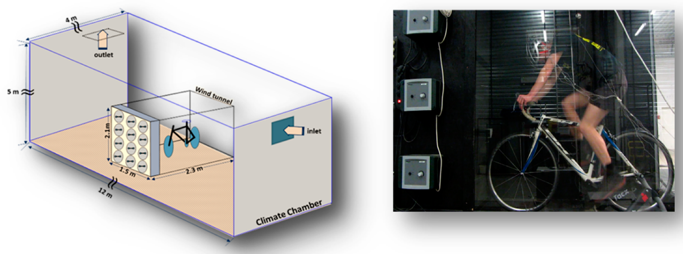
During the course of these experiments, 15 male test subjects with an average age (${\overline{\mu }}_{age}$) of 22 (±1) years and an average weight (${\overline{\mu }}_{mass}$) of 74.3 (±9.2) kg were used in this study. The experimental protocol was approved by the Social and Societal Ethics Committee (SMEC) of KU Leuven. The experiments were conducted using a professional bicycle trainer (Tacx Ironman Smart) with a fastened racing bicycle (BH L52C8 Speedrom) controlling the power delivery of the subject with a power brake. The power brake itself was wirelessly controlled via the Tacx Trainer software. The bicycle trainer was placed in a customised wind tunnel to simulate the wind effect on the test subjects during the course of the experiment (Figure 2). The wind tunnel was 2.1 m high, 2.3 m long and 1.5 m wide. Four rows with three fans each (Fancom type 1435/L7-588 fans) were used as the actuators for wind speed. Each fan produced a maximum ventilation rate of 3000 m³·h⁻¹. A 50 cm long honeycomb gauze structure, placed 25 cm from the fans, was used to obtain a quasi-laminar flow within the open-loop wind tunnel (for more information about the wind tunnel, see [18]). The air speed near the test subject’s head was set to 2.5 m·s⁻¹ to simulate recreational cycling for adults and children. The wind tunnel was placed inside a climate-controlled chamber (Figure 2), the inner dimensions of which were 4 × 11 × 5 m ($w$×$l$×$h$). The air temperature within the climate chamber was controllable within the range of 15–35 °C. Additionally, the ventilation rate within the climate chamber was controllable within the range of 0–2700 m³·h⁻¹ (i.e., 0–11.25 volume refreshments per hour).

2.1.2. Pretest Experiments

The pretest was a modification of the widely used physiological test protocols described by the Australian Institute of Sport [19]. The aim of the pretest was to obtain a power ($P$) value that could be maintained by each of the 15 test subjects for a period of at least 20 min. The maximal lactate steady state (MLSS) and the corresponding workload steady state (WLSS) are presumed to be the maximum workload that can be maintained for endurance sports [20,21]. This lactate threshold is defined as the highest oxygen consumption rate that can be achieved during exercise without a systematic increase in blood lactate concentration [22]. A respiratory exchange ratio (RER) > 1.0 is an indication of the growing contribution of anaerobic metabolism, which causes muscle acidification and leads to muscle fatigue [23].

A bicycle incremental step test was designed in such way that the power increased 30 W every 5 min starting from 100 W. During the test, the subject’s RER was measured with a spirometer (Metamax 3B) and the test was terminated when he exceeded an RER value of 1 for more than 20 s (the corresponding power, $P_{RER = 1}$, was used further in the thermal comfort experiment). The tests were conducted at normal indoor climate conditions with 47% (±4%) relative humidity and an ambient temperature of 20 (±1) °C.

2.1.3. Thermal Comfort and Variable Screening Experimental Protocol

The main objective of this stage was to screen the most suitable variables to predict the cyclist’s under-helmet thermal comfort which can also be easily measured so as to be combatable for smart helmet application. During the course of these experiments, each experimental trial lasted 80 min and was divided into four consecutive timeslots of 20 min each. At each timeslot, a combination of changes in the environmental variables, namely, relative air velocity imposed by the fan ($v$), ambient air temperature ($T_a$), thermal resistance of the scalp ($R_h$) and the delivered cycling power ($P$), was applied. The quantification of the scalp thermal resistance ($R_h$) was developed based on computational fluid dynamic (CFD) simulation for a bare head [24]. The thermal resistance was quantified (see

Table 1. The applied values for each variable.

	${\mathit{T}}_{\mathit{a}}$ (°C)	$\mathit{v}$ (m·s−1)	$\mathit{P}$ (W)	${\mathit{R}}_{\mathit{h} }$(m2·°C·W−1)
Low level	20	0	50% (PRER = 1)	0 (no helmet)
Midlevel	/	/	/	0.045 (with helmet)
High level	30	4	90% (PRER = 1)	0.060 (helmet + aeroshell)

) for the following cases: no-helmet wearing, where $R_h$ was 0; wearing helmet; and wearing helmet with helmet fast (aeroshell). The applied combinations of the different variables with their different levels (low, mid and high) are shown in Table 1.

During the course of each trial, the heart rate ($H_R$), in bpm, of the test subject was measured and logged with a validated heart rate belt sensor (Zephyr^TM bioharness Bt) in combination with a built-in optical heart rate sensor (PPG, Lifebeam) in the bicycle helmet (Lazer Z1 and Lazer Z1 fast = Lazer Z1 + aeroshell). The temperatures of the subject’s forehead, neck, inside of the ear and the air under the bicycle helmet (at front, back, right and left) were continuously measured using calibrated thermocouples (type-T) with a sampling frequency of 1 Hz.

During the experiment, all test subjects were verbally asked about their thermal comfort every 5 min from the start (minute 0) until the end (minute 80) based on the thermal comfort scale introduced by Gagge et al. [10]. For convenience, the cold thermal sensation votes were excluded, as shown in

Table 2. Thermal comfort scale introduced by Gagge et al. [10], excluding the cold sensation votes.

Scale	Thermal Comfort Perception
1	Comfortable
2	Slightly uncomfortable
3	Uncomfortable
4	Very uncomfortable

, as the present work only focused on discomfort perception due to high temperatures.

The experimental design was done using JMP Pro software. A preliminary screening experiment was set up to investigate the contribution of the different variables that, potentially, have an effect on the thermal sensation and thermal comfort under the bicycle helmet. Therefore, each subject was subjected to a combination of different levels of environmental conditions during the experiment.

The experiment was designed to investigate the main effects of the defined environmental input variables, the two-variable interactions between these variables and, due to the particular interest in the effect of a bicycle helmet, the quadratic effect of R_h, which can be mathematically expressed as follows:

$$T_C = {\beta }_{T_a}{T}_a+{\beta }_{R_h}{R}_h+{\beta }_{P}P+{\beta }_{v}v+{\beta }_{Pv}Pv+{\beta }_{P{T}_a}P{T}_a+{\beta }_{P{R}_h}P{R}_h+{\beta }_{R_h{T}_a}{R}_h{T}_a+{\beta }_{R_h{}^2}{R}_h{}^2,$$

(1)

where $T_C$ is the thermal comfort and ${\beta }_i$ is the weighting factor for each variable or variable combination ($i$).

The inclusion of the quadratic effect, which is the interaction effect of the variable with itself, was necessary to generate an experiment that has multiple levels of R_h, so that analysis of a dynamic response due to the bicycle helmet was possible. With the help of the JMP Pro^® software, different combinations (referred to as runs) of the input variables were generated. In general, each participant (test subject) was subjected to four runs (combinations) of the generated ones.

Table 3. Experimental design for test subjects 1 and 8, showing the four runs (combinations) of input variables with three different levels, namely, high (↑), mid (−) and low (↓).

Participant (No. = j)	Variables	Timeslot (1)	Timeslot (2)	Timeslot (3)	Timeslot (4)
$\mathit{j}$ = 1	$T_a$ (°C)	↓	↓	↓	↓
	$v$ (m·s−1)	↑	↓	↑	↓
	$P$ (% PPER = 1)	↓	↓	↑	↑
	$R_h$ (m2·°C·W−1)	−	↑	−	↓
$\mathit{j}$ = 8	$T_a$ (°C)	↑	↑	↑	↑
	$v$ (m·s−1)	↑	↑	↓	↓
	$P$ (% PPER = 1)	↑	↓	↑	↑
	$R_h$ (m2·°C·W−1)	−	−	↓	↑

shows the experimental design for test subjects ($j$) 1 and 8 as an example, where each time slot corresponds to one run (a combination of the four input variables).

2.1.4. General Linear Regression (LR) Model Identification and Offline Parameter Estimation

The main objective of this stage was to identify a general reduced-order and the most parametrically efficient (parsimonious) model structure with the minimum number of easily measured variables (based on the results of the previous stage) to predict the cyclist’s under-helmet thermal comfort. For the sake of the main objective of the present work, the selected predictive model had to be suitable, concerning the computational cost, for wearable sensing technology. Due to the subjective nature of the thermal comfort data, it could not be performed in a continuous pattern, unlike the other input variables, which was a challenge for identifying the predictive model. Hence, in the present paper, we used a simple multivariate regression model with the following general form [25]:

$$T_{ci}=\alpha +{\beta }_1{u}_{i1}+{\beta }_2{u}_{i2}+\dots +{\beta }_m{u}_{im}+{ϵ}_i,\mathrm{for}i \in \left\{1,\dots , n\right\},$$

where $T_{ci}\in ℝ$ is the response (thermal comfort) for the $i$th observation, $\alpha \in ℝ$ is the regression intercept, ${\beta }_j\in ℝ$ is the $j$th predictor’s slope, $u_{ij}\in ℝ$ is the $j$th predictor for the $i$th observation and ${ϵ}_i~N\left(0,{\sigma }^2\right)$ is an independent and identically distributed Gaussian error term. This can be formulated in matrix form as follows:

$${\mathbf{T}}_{\mathbf{C}}=\mathbf{X}\mathit{\beta }+\mathit{ϵ},\mathrm{subjected}\mathrm{to}:{\mathbf{T}}_{\mathbf{C}}\in {ℝ}^{n\times 1}\mathrm{and}\mathbf{X}\in {ℝ}^{n\times m}$$

where $n$ and $m$ are the number of samples and number of predictors (input variables), respectively. In the present paper, we used the ordinary least-squares (OLR) approach to find the regression coefficients estimates ($\widehat{\mathit{\beta }}$) that minimised the sum of the squared errors as follows:

$$\widehat{\mathit{\beta }}=\mathbf{arg}\underset{\mathit{\beta }}{\mathbf{min}}{\left({\mathbf{T}}_{\mathbf{C}}-\mathbf{X}\mathit{\beta }\right)}^{\mathrm{T}}\left({\mathbf{T}}_{\mathbf{C}}-\mathbf{X}\mathit{\beta }\right)={\left({\mathbf{X}}^{\mathrm{T}}\mathbf{X}\right)}^{-1}{\mathbf{X}}^{\mathrm{T}}{\mathbf{T}}_{\mathbf{C}}.$$

2.2. Development of Smart Helmet Prototype

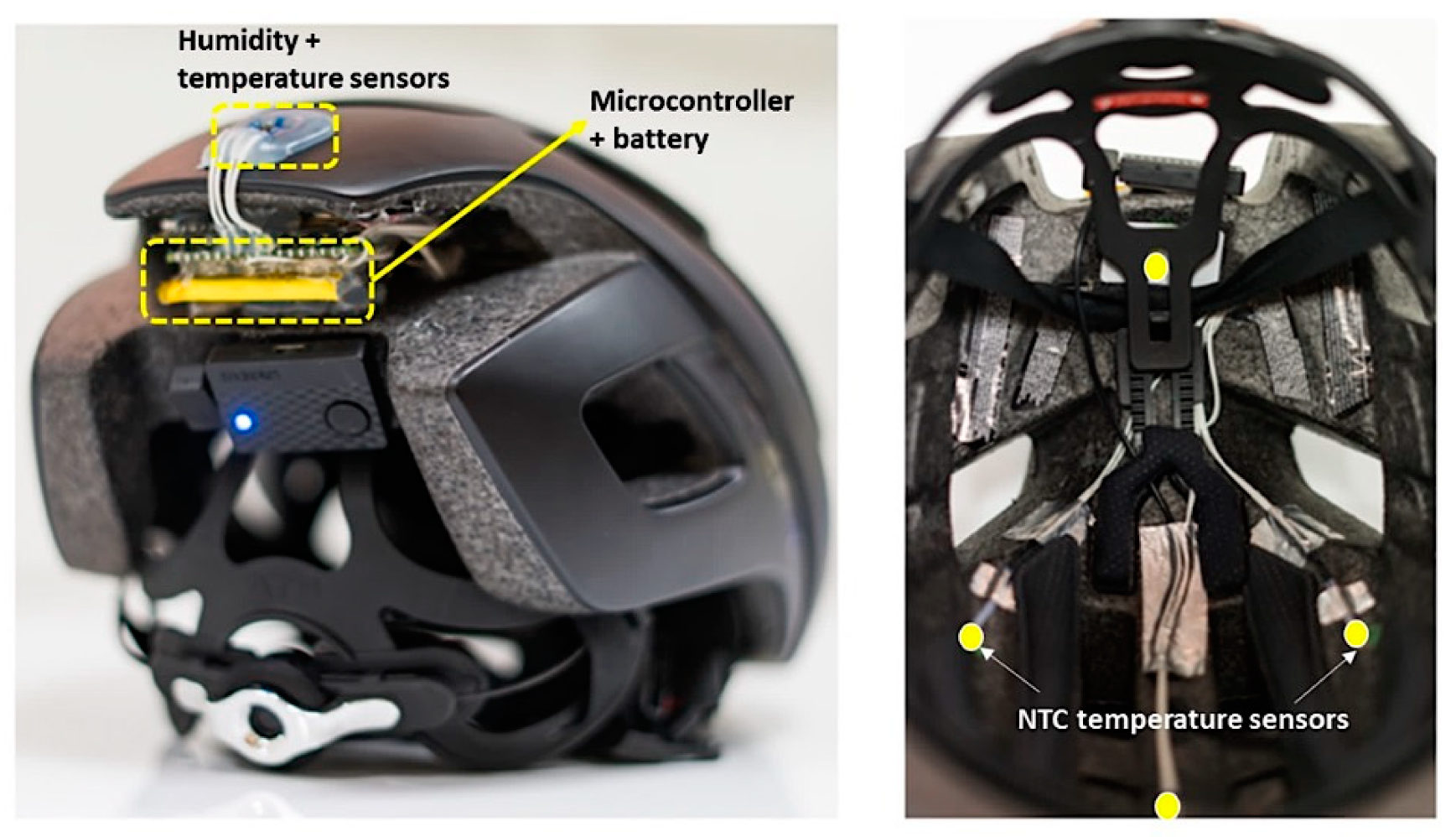
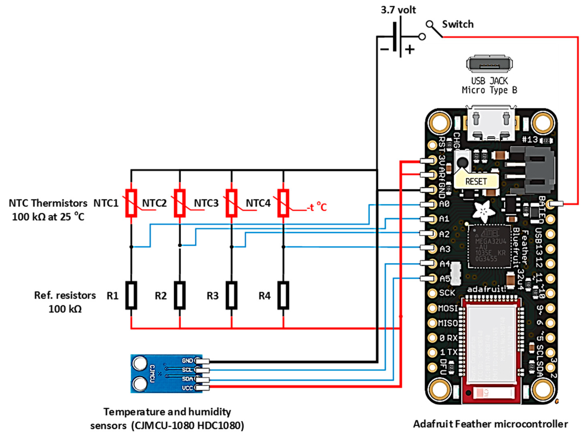
A standard cyclist helmet (312 g) was utilised for the development of the smart helmet prototype (Lazer Bullet 1.0, Lazer Sport, Antwerp, Belgium). The helmet was equipped with a Lifebeam heart rate sensor (Lazer Sport, Antwerp, Belgium; Figure 3) and a 3 × 3 mm digital humidity and temperature sensor (CJMCU-1080 HTC1080, Texas Instruments, Dallas, Texas; accuracy: ±2% for relative humidity and ±0.2 °C for temperature) to measure the surrounding air humidity and temperature. Additionally, four temperature sensors (Negative-Temperature-Coefficient “NTC” temperature sensors, 100 kΩ at 25 °C; Figure 4) were used at the front, back, right and left of the helmet inner body. The final weight of the equipped helmet was 358 g. All sensors were connected directly to a microcontroller (Adafruit Feather 32u4 Bluefruit, Adafruit Industries, New York, NY, USA) that transmitted all data from the helmet to a smartphone via Bluetooth. The Adafruit Bluefruit was chosen as it is the smallest “all-in-one” Arduino-compatible and Bluetooth Low Energy microcontroller with built-in USB and battery charging. The developed system was compatible with a 3.7 V Li-polymer rechargeable battery (LP-523450-1S-3) with the ability to power the system for up to 10 h. A circuit diagram of the used electronics and sensors is shown in Figure 4. The impeded electronics and sensor technology in the smart helmet increased the final original weight of the helmet (312 g) by only 14.7% and did not alter the geometric and aerodynamic characteristics of the original standard helmet. As such, the developed smart helmet is comparable to the original standard helmet (Lazer Bullet 1.0, Lazer Sport, Antwerp, Belgium).

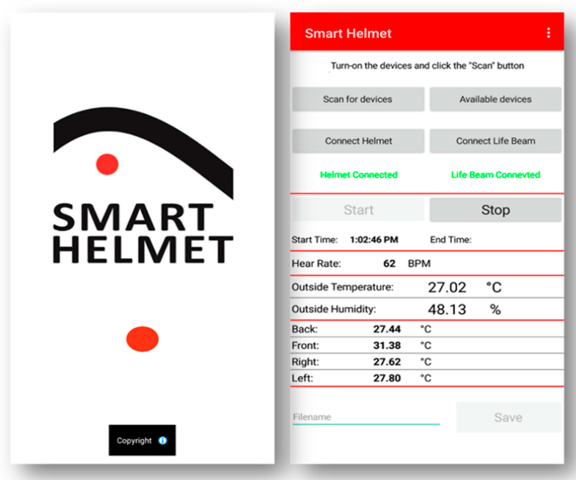
An android-based application “SmartHelmet App” (Figure 5) was developed to simultaneously communicate with both the Adafruit Feather microcontroller and the Lifebeam heart rate monitor via a Bluetooth communication protocol. The SmartHelmet App was developed using the AppyBuilder online platform (App Inventor, Massachusetts Institute of Technology, Cambridge, Massachusetts, USA). The application was designed to receive, display in real-time and store all the data from the SmartHelmet at a 0.2 Hz sampling rate.

2.3. Testing the Developed Smart Helmet Prototype

2.3.1. Test Subjects

In total, seven well-trained male cyclists were recruited for the course of this experiment. Their average physical characteristics were as follows: age—34.5 (±5) years; body mass—74.5 (±7.3) kg; body height—177.6 (±5.4) cm; body mass index (BMI)—23.6 (±1.8) kg∙m⁻²; and body surface area—1.9 (±0.1) m². Prior to the trial, a signed written consent form was obtained from all participants after a detailed description of the protocol, discomforts and benefits. The experimental protocol was approved by the ethical review board at the University of Thessaly, School of Exercise Science in accordance with the recommendations of the Declaration of Helsinki.

2.3.2. Experimental Design and Protocol

Participants were exposed to a hot (34 °C and 56% relative humidity) environment and completed a 30 km cycling time-trial (TT) inside an environmental chamber. In addition, exposure to 800 W of solar radiation was simulated using compact source iodide (CSI) lamps, while a constant wind speed of 5.1 m·s⁻¹ was provided with a large 80 cm diameter industrial fan positioned in front of the participant at a distance of 140 cm from the bicycle saddle. All participants were instructed to abstain from vigorous physical activity 24 h prior the experimental trial and consume at least 500 mL of water and a light meal 2 h before arrival at the laboratory.

Upon arrival at the laboratory, participants changed into their standardised cycling apparel and underwent basic anthropometric measurements. Body height was measured using a stadiometer (Seca 213; Seca GmbH & Co. KG; Hamburg, Germany), while body mass was determined with a digital weighing scale (Version 5.3 KERN & Sohn GmbH). BMI and body surface area were calculated from the measurements of body height and mass. After instrumentation, participants wore the SmartHelmet, entered the controlled environmental chamber and sat on the cycle for 10 min for a baseline period. Thereafter, they performed a 15 min warm-up followed by the 30 km TT. Participants were allowed to drink water ad libitum throughout the TT. No verbal encouragement was provided during the TT.

Cyclists performed the TT on an adjustable friction-braked cycle ergometer (CycleOps 400 Pro Serie Indoor Cycle, Fitchburg, MA, USA), which was combined with the commercially available software Rouvy (VirtualTraining, Vimperk, Czech Republic), allowing simulation of a route on a computer screen. During the 30 km TT, all cyclists were instructed to complete the race as fast as possible with free access to controlling power (W) and cadence (rpm). To simulate real cycling, participants could see their power, cadence and covered distance throughout the TT.

Ratings of perceived exertion (RPE) were reported with the 6–20 point Borg scale [26] before the baseline period, at the beginning of the warm-up period as well as at the start and end times of the TT. Thermal comfort ($T_C$) and thermal sensation ($T_S$) were measured at the same time points using 7- and 9-point scales, respectively [10].

The average power output, pedalling cadence and 30 km TT duration of all the participants (test subjects) are shown in

Table 4. The mean average power output, pedalling cadence and 30 km time-trial (TT) obtained from all test subjects.

Variable	Average (±Standard Deviation)
Power output (W)	176.5 (±24.2)
Cadence (rpm)	93.7 (±14.2)
30 km TT duration (min)	56.9 (±7.9)

.

3. Results

3.1. Pretest Experiments

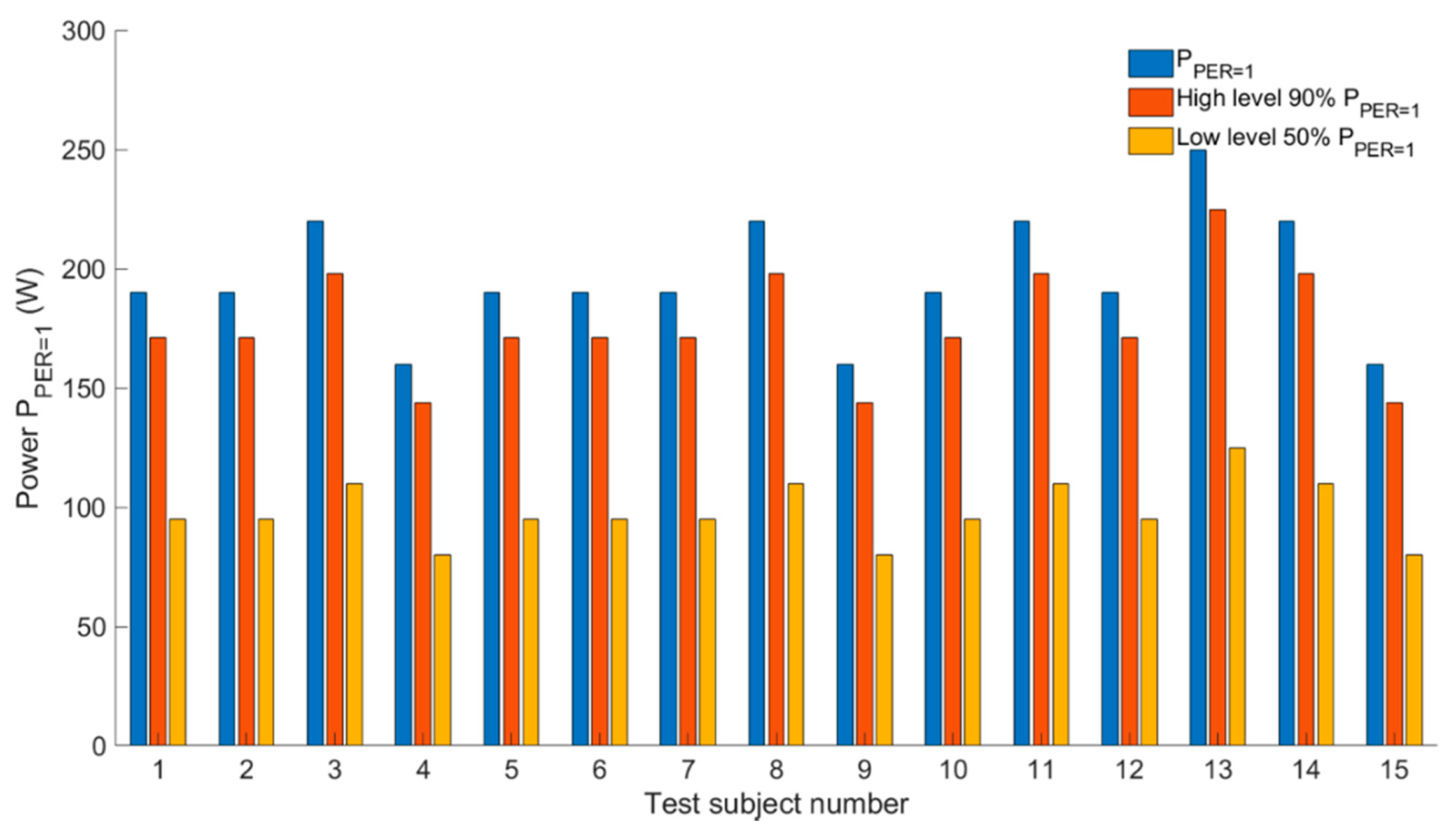
Figure 6 shows the resulting $P_{RER = 1}$ value for each test subject and the corresponding low and high levels of power. The corresponding low ($P$= 50% of $P_{RER = 1}$) and high ($P$ = 90% of $P_{RER = 1}$) levels for each test subject were used in the screening experiments.

3.2. Development of Offline (General) Thermal Comfort Model

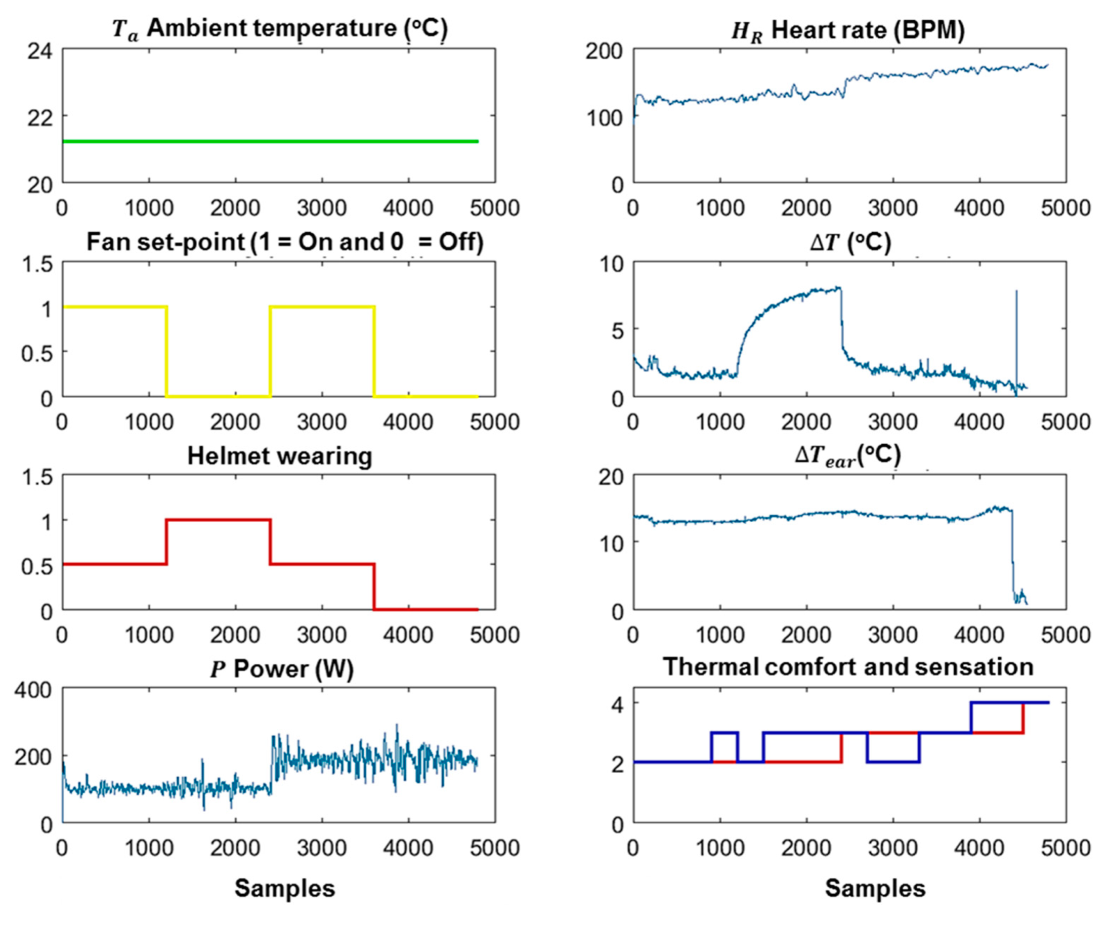
Figure 7 shows the acquired measurements from test subject 1, including environment-related variables, namely, ambient temperature ($T_a$), air velocity ($\mathsf{\nu }$), helmet thermal resistance and applied power level ($R_h$) and the applied mechanical work rate ($P$). Bioresponse-related variables, including heart rate ($H_R$), the temperature difference ($∆T$) between the average temperature beneath the helmet and the ambient air temperature, the temperature difference ($∆T_{ear}$) between the ear temperature and the ambient air temperature as well the thermal comfort ($T_C$), were considered.

The graphs show the environmental variables (left graphs), including the ambient air temperature ($T_a$, °C), fan set-points ($\nu$, 1 = 4 ms⁻¹), the helmet wearing level (0 = no helmet, 0.5 = helmet and 1 = helmet + aeroshell) and the applied mechanical work rate (power) level ($P$, W). The measured variables related to the bioresponses of the test subject (right graphs) were heart rate ($H_R$, bpm), the temperature difference ($∆T$, °C) between the average temperature beneath the helmet and the ambient air temperature, the temperature difference ($∆T_{ear}$, °C) between the ear temperature and the ambient air temperature and the thermal comfort (red line) and sensation (blue line) scores.

To investigate the effect of the different inputs on thermal comfort, different linear regression models (general models) were identified to estimate and predict the perceived under-helmet thermal comfort $T_C$ (output) using continuously measured variables (inputs), including the aforementioned environmental and bioresponse-related variables. The most suitable combination of input variables was selected by retaining only the input variables with a significant (p < 0.05) effect on thermal comfort. Additionally, the best model structure was selected based on two main selection criteria, namely, the goodness of fit ($R^2$) and Akaike information criterion (AIC). The results showed that the most suitable LR model structure, with the highest goodness of fit (average $R^2$ = 0.87 ± 0.05) and lowest Akaike information criterion (average AIC = 138 ± 12), to predict the thermal comfort for all test subjects was as follows:

$$T_C = \alpha +{\beta }_1{T}_a+{\beta }_{2}v+{\beta }_{3}P+{\beta }_4[T_a{R}_h].$$

(2)

The average parameter estimates, t-ratio and p-value of P > |t| for each selected input variable are given in

Table 5. The estimation results of the selected linear regression model (3) to predict thermal comfort, showing the average model estimates for the 15 test subjects.

Term	Parameter	Estimate	Std. Error	t-Ratio	P > |t|
intercept	$\alpha$	2.36	0.14	16.80	<0.0001 *
$T_a$	${\beta }_1$	−0.40	0.11	−3.52	0.0025 *
$v$	${\beta }_2$	−0.36	0.07	−4.85	<0.0001 *
$P$	${\beta }_3$	0.41	0.07	5.45	<0.0001 *
$[T_a{R}_h]$	${\beta }_4$	0.25	0.01	2.52	0.015 *

* significant (p < 0.05).

. The results showed that the main effect of the thermal resistance $R_h$ was not significant (p > 0.05); however, the variable interaction of $R_h$ with $T_a$ showed a significant (p = 0.015) effect on the prediction of the under-helmet thermal comfort.

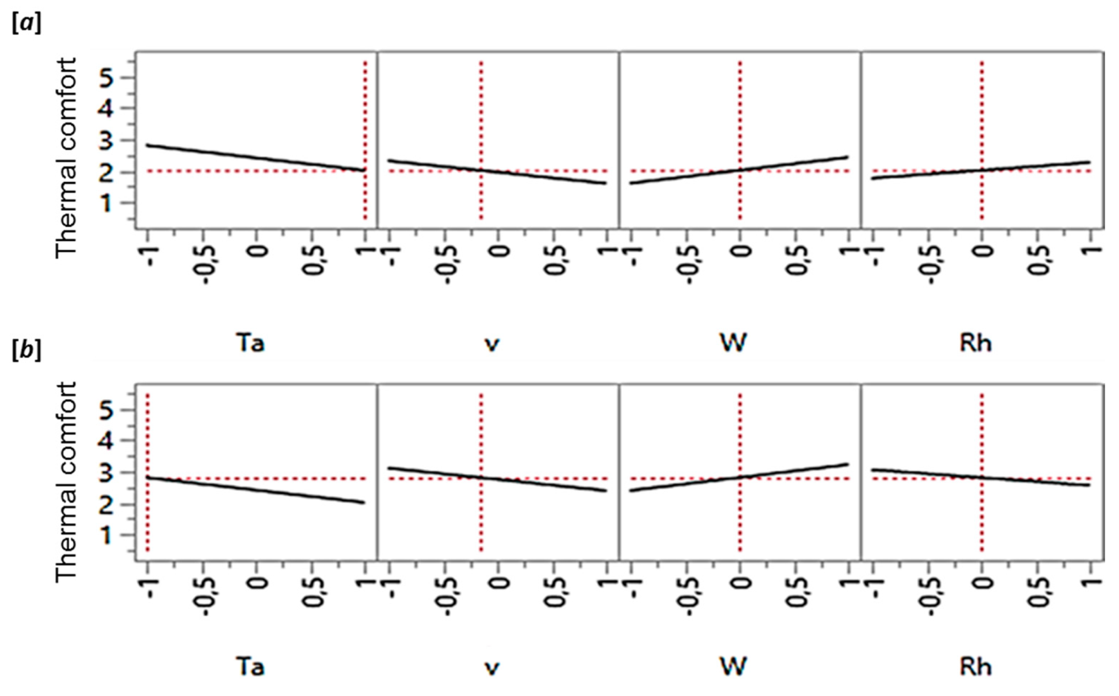
To understand the interaction effect of $R_h$ and $T_a$ on the prediction of thermal comfort, a prediction trace analysis of the model [27] was employed using prediction the JMP^® profiler tool [28], as visualised in Figure 8. For convenience of this analysis, the values of each input variable were scaled (normalised) in such a way to lie in the closed interval [−1, +1], where -1 indicates the variable’s low level and +1 indicates its high level (Figure 8). The scaling of each variable value $i\left(k\right)$ was done according to the following formula:

$$x_i\left(k\right) = \frac{i\left(k\right)-M_i}{{\mathsf{\Delta }}_i}$$

where $x_i\left(k\right)$ is the scaled variable value at time instance $k$, $M_i$ is the midpoint ($M_{i }= \frac{L_i+U_i}{2}$) and $L_i$ and $U_i$ are the particular lower and upper limits of input variable $i$, respectively. The term ${\mathsf{\Delta }}_i$ ($\frac{L_i-U_i}{2}$) is half of the range of the interval.

The prediction trace analysis [28] of the developed model (2) was based on computing the predicted response as one variable was changing while the others were held constant at certain values. The results showed that the effect of $R_h$ was dependent on the level of $T_a$. At a low level (−1) of ambient air temperature ($T_a$ = 20 °C), for a change in thermal resistance $R_h$ from a low level (−1) (i.e., no-bicycle helmet) to a high level (1) (i.e., using the Lazer-Z1 Fast), the predicted thermal comfort scale (Table 2) decreased by 0.5 thermal comfort units but was perceived as comfortable. However, at a high level (1) of ambient air temperature ($T_a$ = 30 °C), the comfort level increased by 0.5 thermal comfort units. This information is important for actively controlling under-helmet thermal comfort, which can be done by manipulating the helmet thermal resistance via, for instance, opening/closing some of the helmet’s holes.

As expected, the heart rate ($H_R$) of the test subjects was found to be highly correlated (Pearson’s correlation coefficient, $r$ = 0.85) with the power ($P$). Additionally, the heart rate was significantly correlated ($r$ = 0.68) with the recorded thermal comfort for all 15 test subjects.

As expected, the temperature difference ($∆T$) between the average air temperature beneath the helmet (${\overline{T}}_h$) and the ambient air temperature ($T_a$) was correlated with both relative air velocity ($\nu$) and helmet thermal resistance ($R_h$), with $r$ = 0.82 and 0.78, respectively.

By employing both heart rate ($H_R$) and the temperature difference ($∆T$) as input variables to the linear regression model, the best model structure that gave the highest average goodness of fit (with average $R^2$ = 0.89 ± 0.04) and lowest Akaike information criterion (average AIC = 123 ± 7) was as follows:

$$T_C = \alpha +{\beta }_1∆T+{\beta }_2{H}_R+{\beta }_3[T_a{R}_h],$$

(3)

where $∆T= {\overline{T}}_h-T_a$ and ${\overline{T}}_h$ is the average air temperature under the helmet, which is calculated from the four temperature sensors located under the helmet. It can be noticed that the structure of model (3) is more compact, consisting of three input variables, compared with the structure of model (2), which consisted of five input variables. Model (3) showed better prediction performance for the thermal comfort level than model (2), which had maximum mean absolute percentage errors (MAPEs) of 8.4% and 11%, respectively. The MAPE is given by

$$MAPE= \frac{100\%}{N}{\displaystyle \sum }_{k=1}^N\left|\frac{{\widehat{T}}_C\left(k\right)-T_C\left(k\right)}{T_C\left(k\right)}\right|$$

where $N$ is the number of data points and ${\widehat{T}}_C$ is the predicted thermal comfort.

It can be noticed that both the mechanical work rate ($P$) and air velocity ($\nu$) disappeared from the compact model (3). The heart rate (H_R) variable included in the compact model (3) directly linked to the applied mechanical work rate ($P$), hence the effect of $P$, included in model (2), translated by the bioresponse represented by H_R (e.g., [29]) included in model (3). According to Newton’s law of cooling, temperature difference ($∆T$) is the driving force for the convective heat transfer ($Q_h$) between the cyclist’s head and the ambient air. The heat flux ($q$) is proportional to $∆T$ and the convective heat transfer coefficient ($h_c$) links both variables as follows:

$$q=-h∆T[\mathrm{W}·\mathrm{m}{}^{-2}].$$

The heat transfer coefficient ($h_c$,W∙m²∙°C) is a combination of the heat transfer coefficient of the air ($h_{air}$) and that of the helmet ($h_H=\frac{1}{R_h}$); hence,

$$\mathsf{\Delta }T=-\left[\frac{1}{h_{air}+\raisebox{1ex}{$1$}\!\left/ \!\raisebox{-1ex}{$R_h$}\right.}\right]q.$$

The heat transfer coefficients of the air ($h_{air}$) and the bicycle helmet ($\raisebox{1ex}{$1$}\!\left/ \!\raisebox{-1ex}{$R_h$}\right.$) are dependent on air velocity ($\nu$). Hence, it is clear that the effect of $\mathsf{\Delta }T$ is inherently connected to the effect of both $\nu$ and helmet thermal resistance ($R_h$).

It can be concluded from the presented results that the input variables included in model (3), namely, temperature difference ($\mathsf{\Delta }T$), heart rate (H_R) of the cyclist and the interaction variable $[T_a{R}_h]$ between ambient temperature ($T_a$) and helmet thermal resistance ($R_h$), were suitable enough to estimate the cyclist’s thermal comfort ($T_C$) under the bicycle helmet. These selected variables were the basis for developing a reduced-order personalised model for real-time monitoring of a cyclist’s thermal comfort under the helmet. Additionally, from a practical point of view, these three variables were suitable to be measured using integrated sensors in the cyclist’s helmet, as is shown in the following subsection.

3.3. Testing the SmartHelmet Prototype and Validation of the Developed General Model

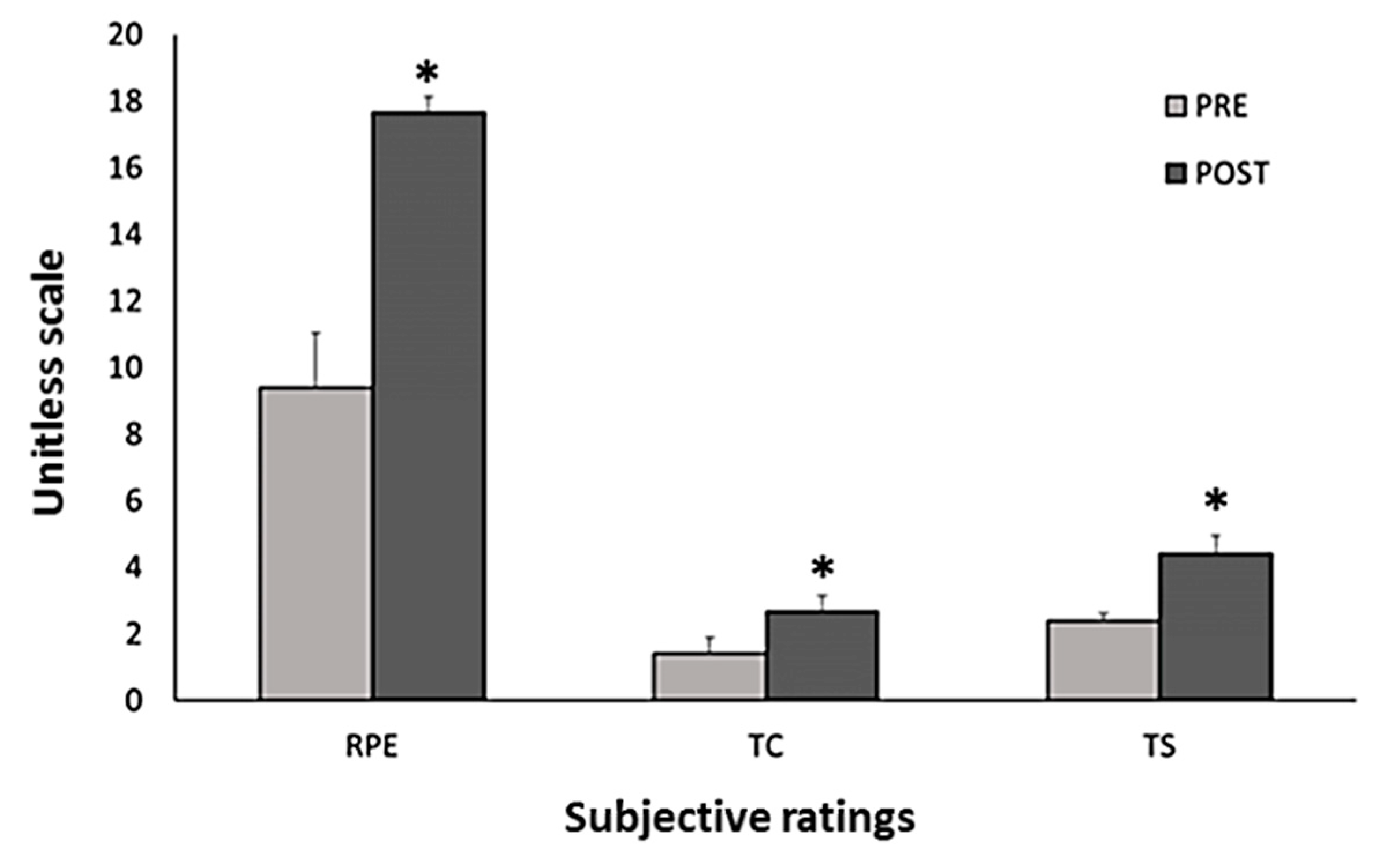
In Figure 9, the average ratings of perceived exertion ($RPE$), thermal comfort ($T_C$) and thermal sensation ($T_S$) values at the start and end times of the TT are presented for all seven test subjects. The average values (±standard deviation) of all used subjective ratings showed a significant (p < 0.05) increase at the end of the TT ($RPE$ = 17.6 ± 0.5, $T_C$ = 2.6 ± 0.5 and $T_S$ = 4.4 ± 0.6) compared with their values at the start of the trial.

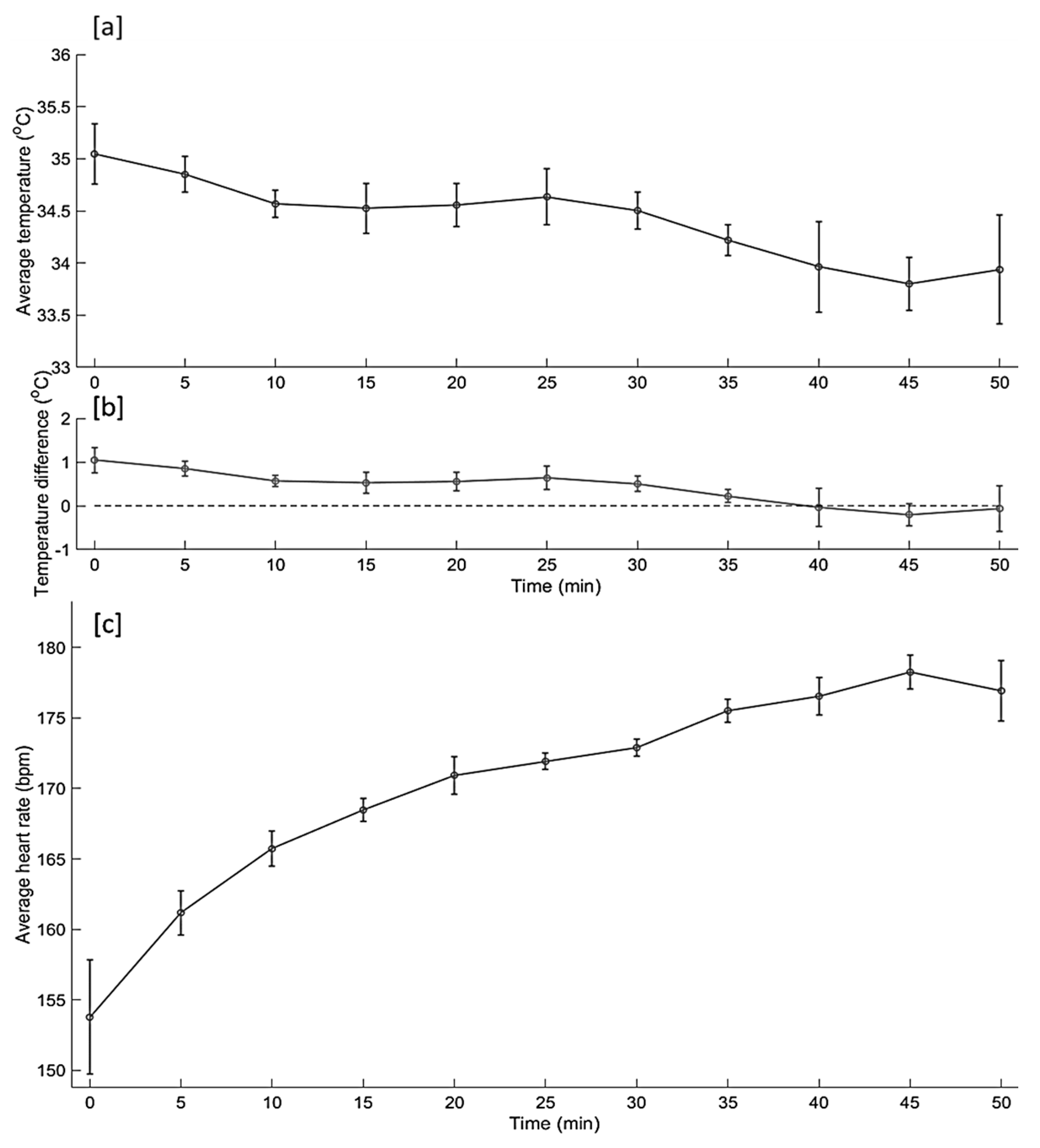
Figure 10 shows the real-time measured average temperatures (${\overline{T}}_h$) under the helmet, average temperature difference ($\Delta T$) between the average temperature under the helmet and the ambient air temperature and the average heart rate (H_R) obtained during the TT from all seven test subjects using the developed prototype smart helmet.

The developed offline liner regression model (3) was used to estimate the thermal comfort ($T_C$) of all seven test subjects based on the measurements acquired from the SmartHelmet prototype and for comparison with the thermal comfort subjective rating. The model was able to estimate the thermal comfort from all test subjects and revealed an average $R^2$ of 0.84 (±0.03). Model (3) was able to predict the cyclist’s thermal comfort under the helmet and had a maximum MAPE of 10%. However, by retuning the model parameters using the data obtained from the TT experiment, the maximum MAPE was reduced to 7.8%.

The main advantage of the proposed model is that it is a conceptually simple yet very effective tool to explore linear relationships between a response variable (output) and a set of explanatory variables (input variables), which can be easily used for wearable technology such as the SmartHelmet. On the other hand, the disadvantage of such a model is the absence of the time component; in other words, the model is not able to explain the transient response of the output. Additionally, in practice, many factors can affect and change the relationship represented by the proposed model. These factors include helmet-related factors (e.g., helmet weight), other environmental conditions (e.g., wind direction) and personal-related factors, which were not included in the model (e.g., the surface area and contour of the cyclist’s head). Hence, it is clear that such general models need to be adapted to new data (personal data) and different conditions for better performance. With the help of wearable sensing technologies (SmartHelmet) and streaming modelling algorithms, an adaptive personalised model can be developed for real-time monitoring of a cyclist’s head thermal comfort.

In the following subsection, we introduce the framework of online model adaptation and personalisation (streaming algorithm) based on the easily measured variables obtained from the wearable sensors impeded in the SmartHelmet.

3.4. Introduction of Online Personalisation and Adaptive Modelling Algorithm

Most of the available thermal sensation and comfort predictive models (e.g., [30,31,32,33,34,35,36,37]) are static models. That is, they predict the average vote of a large group of people based on, for example, the 7-point thermal sensation scale instead of individual thermal comfort, and they only describe the overall thermal sensation/comfort of multiple occupants in a shared thermal environment. To overcome the disadvantages of static models, adaptive thermal comfort models aim to provide insights and opportunities to personalise the thermal comfort prediction of individuals [38]. The idea behind adaptive models is that occupants and individuals are no longer regarded as passive recipients of the thermal environment, but rather, they play an active role in creating their own thermal preferences [39]. The suggested linear regression model, represented by (3), in the present paper is considered as a global model, also called an offline model [40,41], for an adaptive personalised model to assess and predict individual thermal comfort under a cyclist’s helmet.

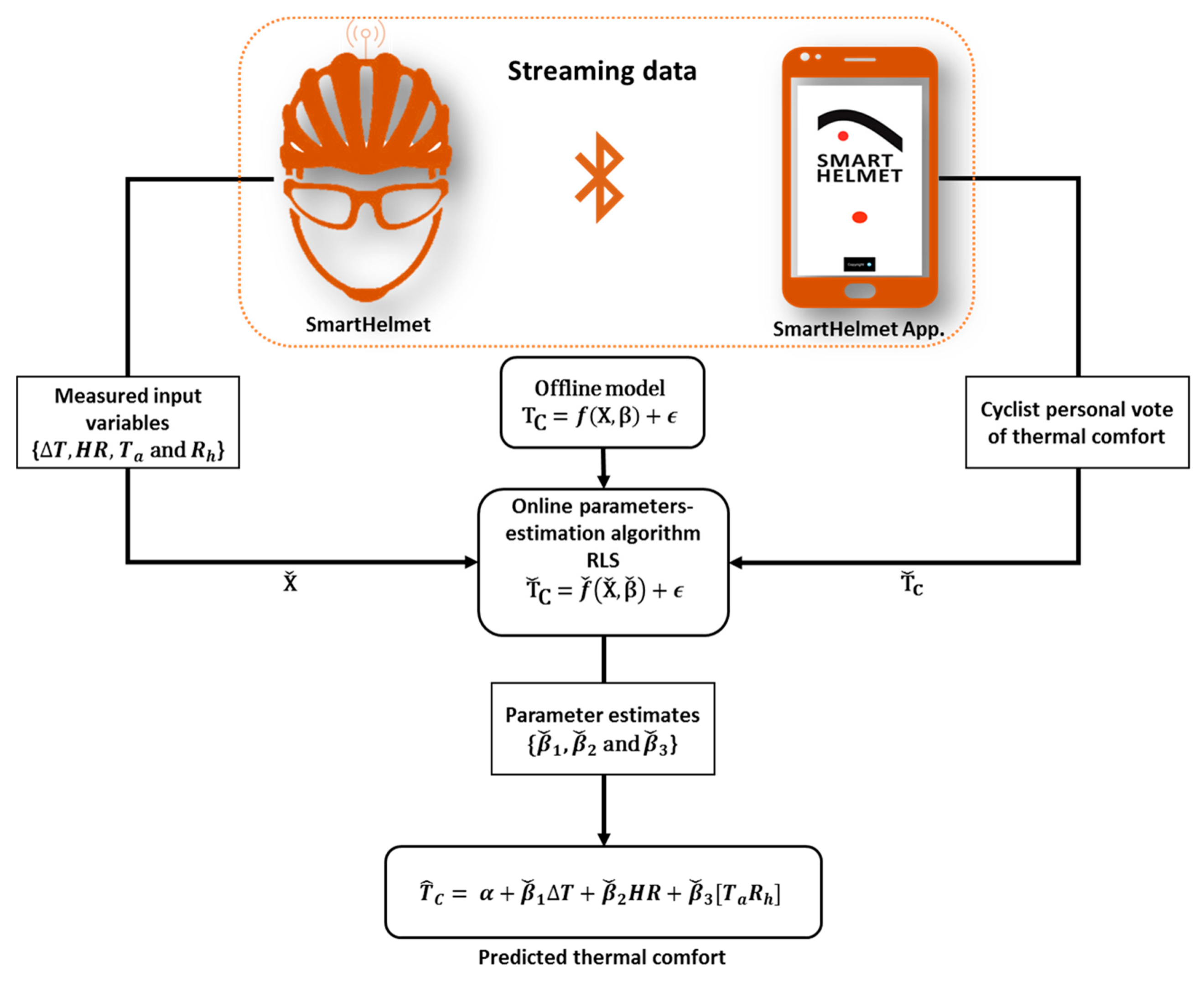
Figure 11 depicts the proposed steps for retuning and personalising the offline regression model (3). The suggested personalised adaptive tuning algorithm consists of the main components shown in Figure 11.

3.4.1. Offline Linear Regression Model

As mentioned earlier, the linear regression model (3), which was developed based on the data obtained from the 15 test subjects, is the offline base model for online prediction of personal under-helmet thermal comfort. The general form of the offline linear regression model (3) is as follows:

$${\mathbf{T}}_{\mathbf{C}}=\mathbf{X}\mathit{\beta }+\mathit{ϵ}$$

(4)

and is subjected to ${\mathbf{T}}_{\mathbf{C}}\in {ℝ}^{n\times 1}$ and $\mathbf{X}\in {ℝ}^{n\times 3}$,where ${\mathbf{T}}_{\mathbf{C}}$ is the output vector ($n$ samples of thermal comfort votes$)$; $\mathit{ϵ}$ is the model residual vector, which consists of independent and Gaussian-distributed entries; and $\mathit{\beta }$ and $\mathbf{X}$ are the regression vector (of the size 3) and predictor matrix (of the size $n\times 3$), respectively, given by

$$\mathbf{X}= \left[\begin{array}{ccc}\begin{array}{cc}1& ∆T_1\end{array}& H_R{}_1& {\left(T_a{R}_h\right)}_1\\ \begin{array}{c}\begin{array}{cc}1& ∆T_2\end{array}\\ \begin{array}{cc}⋮ & ⋮\end{array}\end{array}& \begin{array}{c}{H}_R{}_2\\ ⋮\end{array}& \begin{array}{c}{\left(T_a{R}_h\right)}_2\\ ⋮\end{array}\\ \begin{array}{cc}1& ∆T_n\end{array}& H_R{}_n& {\left(T_a{R}_h\right)}_n\end{array}\right]\mathrm{and}\mathit{\beta }=\left[\begin{array}{c}\begin{array}{c}\alpha \\ {\beta }_1\end{array}\\ {\beta }_2\\ {\beta }_3\end{array}\right].$$

3.4.2. Streaming Data

The availability of real-time sensor data from the developed SmartHelmet prototype allows for streaming data, which is processed via an online algorithm (stream processing) to adapt the offline model [42]. The streaming data includes new $\check{n}$ samples of measured sensor data (new input matrix $\check{\mathbf{X}}$) acquired from the SmartHelmet sensors, and new personal thermal comfort votes (new output vector ${\check{\mathbf{T}}}_{\mathbf{C}}$) acquired through an interactive query provided by the developed SmartHelmet App.

3.4.3. Online Parameter Estimation Algorithm

As explained earlier (Section 2.1.3), the general setting of regression analysis is to identify a relationship between a response variable ($Y$) and one or several explanatory variables (predictors) ($X$) by using a learning sample [43]. In a prediction framework, the main assumption for predicting $Y$ on a new sample of $X$observations is that the regression model (with the general form $Y = f\left(X\right) + ϵ$, where $ϵ$ represents the model residuals) is still valid. Unfortunately, this assumption is not valid in the present case, where the thermal comfort of the individual cyclist is strongly dependent on many personal- and time-dependent factors [11]. Therefore, in this study, we adapted the original regression model (3) to a new sample (observations) by estimating a transformation [41,43] between the original regression function ($f\left(X\right)$) and the new one ($\check{f}(\check{X})$) while still using the same model variables and structure. Ordinary least squares (LS) is one of the most popular regression techniques, which was used here for parameter estimation of the developed offline model. However, for the online parameter estimation and in the presence of unknown parameter changes, its adaptive versions—the sliding or moving LS, recursive least squares (RLS) and recursive partial least squares (PLS)—are widely used [41,44,45].

In the present paper, the RLS algorithm is suggested for online personalisation and adaptive modelling of under-helmet thermal comfort. The suggested RLS algorithm has the advantage of being simple and computationally efficient for wearable and adaptive sensing, which was the case in the present work. In the RLS algorithm, the new regression vector $\check{\mathit{\beta }}$, as in Equation (4), can be estimated recursively as follows [25,46,47]:

$${\mathbf{P}}_{n+1}={\mathbf{P}}_n-\frac{{\mathbf{P}}_{\mathbf{n}}{\left({\mathbf{X}}_{n+1}\right)}^T{\mathbf{X}}_{n+1}{\mathbf{P}}_n}{1+{\mathbf{X}}_{n+1}{\mathbf{P}}_n{\left({\mathbf{X}}_{n+1}\right)}^T},$$

(5)

$${\check{\mathit{\beta }}}_{n+1}={\check{\mathit{\beta }}}_n+{\mathbf{P}}_{n+1}{\left({\mathbf{X}}_{n+1}\right)}^T\left({\check{\mathit{T}}}_{{\mathit{C}}_{\mathit{n}\mathbf{+}\mathbf{1}}}-{\mathbf{X}}_{n+1}{\check{\mathit{\beta }}}_n\right)$$

(6)

where ${\mathbf{P}}_n={\left({\mathbf{X}}_n{}^T{\mathbf{X}}_n\right)}^{-1}$. This recursive algorithm is efficient for cases where the regression vector $\check{\mathit{\beta }}$ is a function of time (time varying). However, in the case of adaptive modelling with streaming data, due to the arrival of new samples, the influence of new observations decreases gradually and the ability to track the changes in $\check{\mathit{\beta }}$ will be lost. Hence, to mitigate this, the widely used and popular forgetting factor approach [48] is proposed in this paper. The approach of forgetting here is based on gradually discarding older data in favour of more recent information. In the least-squares method, forgetting can be viewed as giving less weight to older data and more weight to recent data [48,49]. Hence, the forgetting factor, $\lambda$, was introduced to (5) as follows [41]:

$${\mathbf{P}}_{n+1}=\frac{1}{\lambda }\left({\mathbf{P}}_n-\frac{{\mathbf{P}}_{\mathbf{n}}{\left({\mathbf{X}}_{n+1}\right)}^T{\mathbf{X}}_{n+1}{\mathbf{P}}_n}{\lambda +{\mathbf{X}}_{n+1}{\mathbf{P}}_n{\left({\mathbf{X}}_{n+1}\right)}^T}\right)$$

(7)

where $\lambda \in \left(0, 1\right]$. The forgettiing factor $\lambda$ operates as a weight, which diminishes for more remote data and expands for more recent data [48,49]. The main difference here between (5) and (7) is that in conventional RLS (5), the covariance vanishes to zero with time, losing its capability to keep track of changes in the regression vector $\check{\mathit{\beta }}$. In (7), however, the covariance matrix is divided by $0\le \lambda <1$ at each update. This slows down the fading out of the covariance matrix [49].

4. Conclusions

In the present work, we aimed to develop a general model approach to predict a cyclist’s head thermal comfort using nonintrusive and easily measured variables, which can be measured using impeded sensors in a bicycle helmet. During the first experimental stage, 15 participants were exposed to different levels of mechanical activity, ambient temperatures, helmet thermal resistance and wind velocities in order to develop a general model to predict a cyclist’s head thermal comfort. The results showed that ambient temperature, average air temperature under the helmet, cyclist heart rate, cyclist mechanical work and helmet thermal resistance significantly influenced the cyclist’s head thermal comfort. A reduced-order general linear regression model with three input variables, namely, temperature difference between ambient temperature and average under-helmet temperature, cyclist’s heart rate and the interaction between ambient temperature and helmet thermal resistance, was the most suitable to predict the cyclist’s head thermal comfort, showing a maximum MAPE of 8.4%. The developed general model structure was based on easily measured variables that can be measured continuously using impeded sensors in the bicycle helmet but is still of reduced order and low computational cost, which is suitable for streaming and adaptive modelling. Based on the selected model variables, a smart helmet prototype (SmartHelmet) was developed using impeded sensing technology as a proof of concept. The developed general model was validated using the developed SmartHelmet prototype. During the validation experimental phase, seven well-trained male cyclists were exposed to a hot (34 °C and 56% relative humidity) environment and completed a 30 km cycling TT inside an environmental chamber. The validation results showed that the developed general model was able to predict the thermal comfort of the seven participants and had a maximum MAPE of 10%. By retuning the model parameters, the maximum MAPE decreased to 7.8%. Finally, we introduced a calculation framework of an adaptive personalised model based on the developed general model to predict a cyclist’s head thermal comfort based on streaming data from the SmartHelmet prototype.

References

1. Titze, S.; Bauman, A.; De Geus, B.; Krenn, P.; Kohlberger, T.; Reger-Nash, B.; Oja, P. Health benefits of cycling: A systematic review. Scand. J. Med. Sci. Sports 2011, 21, 496–509. [Google Scholar]
2. Zentner, J.; Franken, H.; Löbbecke, G. Head injuries from bicycle accidents. Clin. Neurol. Neurosurg. 1996, 98, 281–285. [Google Scholar] [CrossRef]
3. Elvik, R. Publication bias and time-trend bias in meta-analysis of bicycle helmet efficacy: A re-analysis of Attewell, Glase and McFadden, 2001. Accid. Anal. Prev. 2011, 43, 1245–1251. [Google Scholar] [CrossRef] [PubMed]
4. Action, A.C.; Hope, T.U. Final Report of Working Group 2: Traffic Psychology; COST Action TU1101/HOPE: Brussels, Belgium, 2015. [Google Scholar]
5. Finnoff, J.T.; Laskowski, E.R.; Altman, K.L.; Diehl, N.N. Barriers to Bicycle Helmet Use. Pediatrics 2001, 108, 2–10. [Google Scholar] [CrossRef] [PubMed]
6. Bogerd, C.P.; Aerts, J.M.; Annaheim, S.; Bröde, P.; De Bruyne, G.; Flouris, A.D.; Kuklane, K.; Mayor, T.S.; Rossi, R.M. A review on ergonomics of headgear: Thermal effects. Int. J. Ind. Ergon. 2015, 45, 1–12. [Google Scholar] [CrossRef] [Green Version]
7. Underwood, L.; Vircondelet, C.; Jermy, M. Thermal comfort and drag of a streamlined cycling helmet as a function of ventilation hole placement. Proc. Inst. Mech. Eng. Part P J. Sports Eng. Technol. 2018, 232, 15–21. [Google Scholar] [CrossRef]
8. Mayor, T.S.; Couto, S.; Psikuta, A.; Rossi, R.M. Advanced modelling of the transport phenomena across horizontal clothing microclimates with natural convection. Int. J. Biometeorol. 2015, 59, 1875–1889. [Google Scholar] [CrossRef] [PubMed]
9. ASHRAE. ASHRAE Standard 55; American Society of Heating, Refrigerating and Air-Conditioning Engineers, Inc.: Atlanta, GA, USA, 2017. [Google Scholar]
10. Gagge, A.P.; Stolwijk, J.A.J.; Hardy, J.D. Comfort and thermal sensations and associated physiological responses at various ambient temperatures. Environ. Res. 1967, 1, 1–20. [Google Scholar] [CrossRef]
11. Kenneth, C. Human Thermal Environments: The Effects of Hot, Moderate, and Cold Environments on Human Health, Comfort, and Performance, 3rd ed.; CRC Press: Boca Raton, FL, USA, 2014. [Google Scholar]
12. Fanger, P.O. Thermal Comfort: Analysis and Applications in Environmental Engineering, 1st ed.; Danish Technical Press: Lyngby, Denmark, 1970. [Google Scholar]
13. Enescu, D. Models and Indicators to Assess Thermal Sensation Under Steady-state and Transient Conditions. Energies 2019, 12, 841. [Google Scholar] [CrossRef]
14. Koelblen, B.; Psikuta, A.; Bogdan, A.; Annaheim, S.; Rossi, R.M. Thermal sensation models: A systematic comparison. Indoor Air 2017, 27, 680–689. [Google Scholar] [CrossRef]
15. Rugh, J.P.; Farrington, R.B.; Bharathan, D.; Vlahinos, A.; Burke, R.; Huizenga, C.; Zhang, H. Predicting human thermal comfort in a transient nonuniform thermal environment. Eur. J. Appl. Physiol. 2004, 92, 721–727. [Google Scholar] [CrossRef] [Green Version]
16. Havenith, G.; Fiala, D. Thermal Indices and Thermophysiological Modeling for Heat Stress. Compr. Physiol. 2015, 6, 255–302. [Google Scholar]
17. Youssef, A.; Truyen, P.; Brode, P.; Fiala, D.; Aerts, J.M. Towards Real-Time Model-Based Monitoring and Adoptive Controlling of Indoor Thermal Comfort. In Proceedings of the Ventilating Healthy Low-Energy Buildings, Nottingham, UK, 13–14 September 2017. [Google Scholar]
18. De Bruyne, G.; Aerts, J.M.; Sloten, J.V.; Goffin, J.; Verpoest, I.; Berckmans, D. Quantification of local ventilation efficiency under bicycle helmets. Int. J. Ind. Ergon. 2012, 42, 278–286. [Google Scholar] [CrossRef]
19. Gore, C.J. Physiological Tests for Elite Athletes Australian Sports Commmission; Human Kinetics: Champaign, IL, USA, 2000. [Google Scholar]
20. Biochemistry, B.B.; Science, S. The Concept of Maximal Lactate Steady State. Sports Med. 2003, 33, 407–426. [Google Scholar]
21. Beneke, R. Methodological aspects of maximal lactate steady state-implications for performance testing. Eur. J. Appl. Physiol. 2003, 89, 95–99. [Google Scholar] [CrossRef]
22. Sibernagl, S. Atlas van de Fysiologie; SESAM/HBuitgevers: Baarn, The Netherlands, 2008. [Google Scholar]
23. Fitts, R.H. Cellular mechanisms of muscle fatigue. Physiol. Rev. 1994, 74, 49–94. [Google Scholar] [CrossRef]
24. Mukunthan, S.; Vleugels, J.; Huysmans, T.; de Bruyne, G. Latent Heat Loss of a Virtual Thermal Manikin for Evaluating the Thermal Performance of Bicycle Helmets. In Advances in Human Factors in Simulation and Modeling; Springer: Cham, Switzerland, 2019; pp. 66–78. [Google Scholar]
25. Soong, T.T. Fundamentals of Probability and Statistics for Engineers; Wiley: Hoboken, NJ, USA, 2004. [Google Scholar]
26. Borg, G.A. Psychophysical bases of perceived exertion. Med. Sci. Sports Exerc. 1982, 14, 377–381. [Google Scholar] [CrossRef]
27. Box, G.E.P.; Draper, N.R. Empirical Model-Building and Response Surfaces; John Wiley & Sons: Oxford, UK, 1987. [Google Scholar]
28. JMP® 14. JMP® 14 Profilers; Institute Inc.: Cary, NC, USA, 2018. [Google Scholar]
29. Zinoubi, B.; Zbidi, S.; Vandewalle, H.; Chamari, K.; Driss, T. Relationships between rating of perceived exertion, heart rate and blood lactate during continuous and alternated-intensity cycling exercises. Biol. Sport 2018, 35, 29–37. [Google Scholar] [CrossRef]
30. Takada, S.; Matsumoto, S.; Matsushita, T. Prediction of whole-body thermal sensation in the non-steady state based on skin temperature. Build. Environ. 2013, 68, 123–133. [Google Scholar] [CrossRef]
31. Fiala, D. Dynamic Simulation of Human Heat Transfer and Thermal Comfort; De Montfort University: Leicester, UK, 1998. [Google Scholar]
32. Lomas, K.J.; Fiala, D.; Stohrer, M. First principles modeling of thermal sensation responses in steady-state and transient conditions. ASHRAE Trans. 2003, 109, 179–186. [Google Scholar]
33. Zhang, H. Human Thermal Sensation and Comfort in Transient and Non-Uniform Thermal Environments; University of California: Berkeley, CA, USA, 2003. [Google Scholar]
34. Guan, Y.D.; Hosni, M.H.; Jones, B.W.; Gielda, T.P. Investigation of Human Thermal Comfort Under Highly Transient Conditions for Automotive Applications-Part 2: Thermal Sensation Modeling. ASHRAE Trans. 2003, 109, 898–907. [Google Scholar]
35. Guan, Y.D.; Hosni, M.H.; Jones, B.W.; Gielda, T.P. Investigation of Human Thermal Comfort Under Highly Transient Conditions for Automotive Applications-Part 1: Experimental Design and Human Subject Testing Implementation. ASHRAE Trans. 2003, 109, 885–897. [Google Scholar]
36. Nilsson, H.O.; Holmer, I. Comfort climate evaluation with thermal manikin methods and computer simulation models. Indoor Air 2003, 13, 28–37. [Google Scholar] [CrossRef]
37. Kingma, B.R.M.; Schellen, L.; Frijns, A.J.H.; Lichtenbelt, W.D.V. Thermal sensation: A mathematical model based on neurophysiology. Indoor Air 2012, 22, 253–262. [Google Scholar] [CrossRef]
38. Lu, S.; Wang, W.; Wang, S.; Hameen, E.C. Thermal Comfort-Based Personalized Models with Non-Intrusive Sensing Technique in Office Buildings. Appl. Sci. 2019, 9, 1768. [Google Scholar] [CrossRef]
39. De Dear, R.; Brager, G.S. Developing an adaptive model of thermal comfort and preference. ASHRAE Trans. 1998, 104, 145–167. [Google Scholar]
40. Kadlec, P.; Grbić, R.; Gabrys, B. Review of adaptation mechanisms for data-driven soft sensors. Comput. Chem. Eng. 2011, 35, 1–24. [Google Scholar] [CrossRef]
41. Sharma, S.; Khare, S.; Huang, B. Robust online algorithm for adaptive linear regression parameter estimation and prediction. J. Chemom. 2016, 30, 308–323. [Google Scholar] [CrossRef]
42. Zimmer, A.M.; Kurze, M.; Seidl, T. Adaptive Model Tree for Streaming Data. In Proceedings of the 2013 IEEE 13th International Conference on Data Mining, Dallas, TX, USA, 7–10 December 2013; pp. 1319–1324. [Google Scholar]
43. Bouveyron, C.; Jacques, J. Adaptive linear models for regression: Improving prediction when population has changed. Pattern Recognit. Lett. 2010, 31, 2237–2247. [Google Scholar] [CrossRef] [Green Version]
44. Jiang, J.; Zhang, Y. A revisit to block and recursive least squares for parameter estimation. Comput. Electr. Eng. 2004, 30, 403–416. [Google Scholar] [CrossRef]
45. Young, P.C. Recursive Estimation and Time-Series Analysis; Springer: Berlin, Germany, 2011. [Google Scholar]
46. Benesty, J.; Paleologu, C.; Gänsler, T.; Ciochină, S. Recursive Least-Squares Algorithms; Springer: Berlin, Germany, 2011; pp. 63–69. [Google Scholar]
47. Plackett, R.L. Some Theorems in Least Squares. Biometrika 1950, 37, 149. [Google Scholar] [CrossRef]
48. Johnson, C.R. Lectures on Adaptive Parameter Estimation; Prentice-Hall: Upper Saddle River, NJ, USA, 1988. [Google Scholar]
49. Vahidi, A.; Stefanopoulou, A.; Peng, H. Recursive least squares with forgetting for online estimation of vehicle mass and road grade: Theory and experiments. Veh. Syst. Dyn. 2005, 43, 31–55. [Google Scholar] [CrossRef]
Figure 1. Schematic diagram showing the general framework of the development of a personalised adaptive model for the smart helmet prototype.
Applsci 09 03170 g001
Figure 2. Schematic representation showing the used bicycle fixed inside a customised wind tunnel and placed within a climate chamber (left) and a photograph of a test subject riding the bike within the wind tunnel (right).
Applsci 09 03170 g002
Figure 3. The developed smart helmet prototype showing the microcontroller and the humidity and temperature sensor on the back side of the helmet (left picture) and the four NTC temperature sensors placed in the inner body of the helmet (right picture).
Applsci 09 03170 g003
Figure 4. Circuit diagram of the stand-alone sensor system impeded in the smart helmet prototype.
Applsci 09 03170 g004
Figure 5. A screenshot of the designed SmartHelmet App.
Applsci 09 03170 g005
Figure 6. Obtained power values of the pretest. These power values correspond to the power value when they exceeded a respiratory exchange ratio (RER) of one.
Applsci 09 03170 g006
Figure 7. The recorded measurements of the different variables obtained from test subject 1.
Applsci 09 03170 g007
Figure 8. Visualisation of the model prediction traces showing the interaction effect of the thermal resistance ( R h ) and ambient temperature ( T a ) on the predicted thermal comfort. (a) When the temperature was low (20 °C), additional thermal resistance was perceived as comfortable. However, (b) when the temperature was high (30 °C), additional thermal resistance was perceived as uncomfortable. The values of the input variables were normalised in the range between -1 and 1, which correspond to low and high levels, respectively. Table 6 shows the average parameter estimates of the developed compact regression model (3) for the 15 test subjects.
Applsci 09 03170 g008
Figure 9. Average values of ratings of perceived exertion (RPE), thermal comfort ( T C ) and thermal sensation ( T S ) between the start (PRE) and end (POST) times of the TT (* indicates a significant difference of p < 0.05).
Applsci 09 03170 g009
Figure 10. (a) Average temperature ( T ¯ h ) beneath the helmet, (b) average temperature difference ( Δ T ) between the average temperature and the ambient air temperature and (c) average heart rate (HR) obtained during the TT from all test subjects.
Applsci 09 03170 g010
Figure 11. Schematic representation of the proposed online personalisation algorithm to predict thermal comfort under the helmet. The retuning and personalisation algorithm is based on data streaming obtained from the developed SmartHelmet prototype and the cyclist’s personal vote of thermal comfort acquired from the developed SmartHelmet App. The streamed data is fed, together with the developed offline model, to an online parameter estimation algorithm based on a recursive least-squares (RLS) algorithm.
Applsci 09 03170 g011