Towards Model-Based Online Monitoring of Cyclist’s Head Thermal Comfort: Smart Helmet Concept and Prototype


Abstract
Featured Application
Abstract
1. Introduction
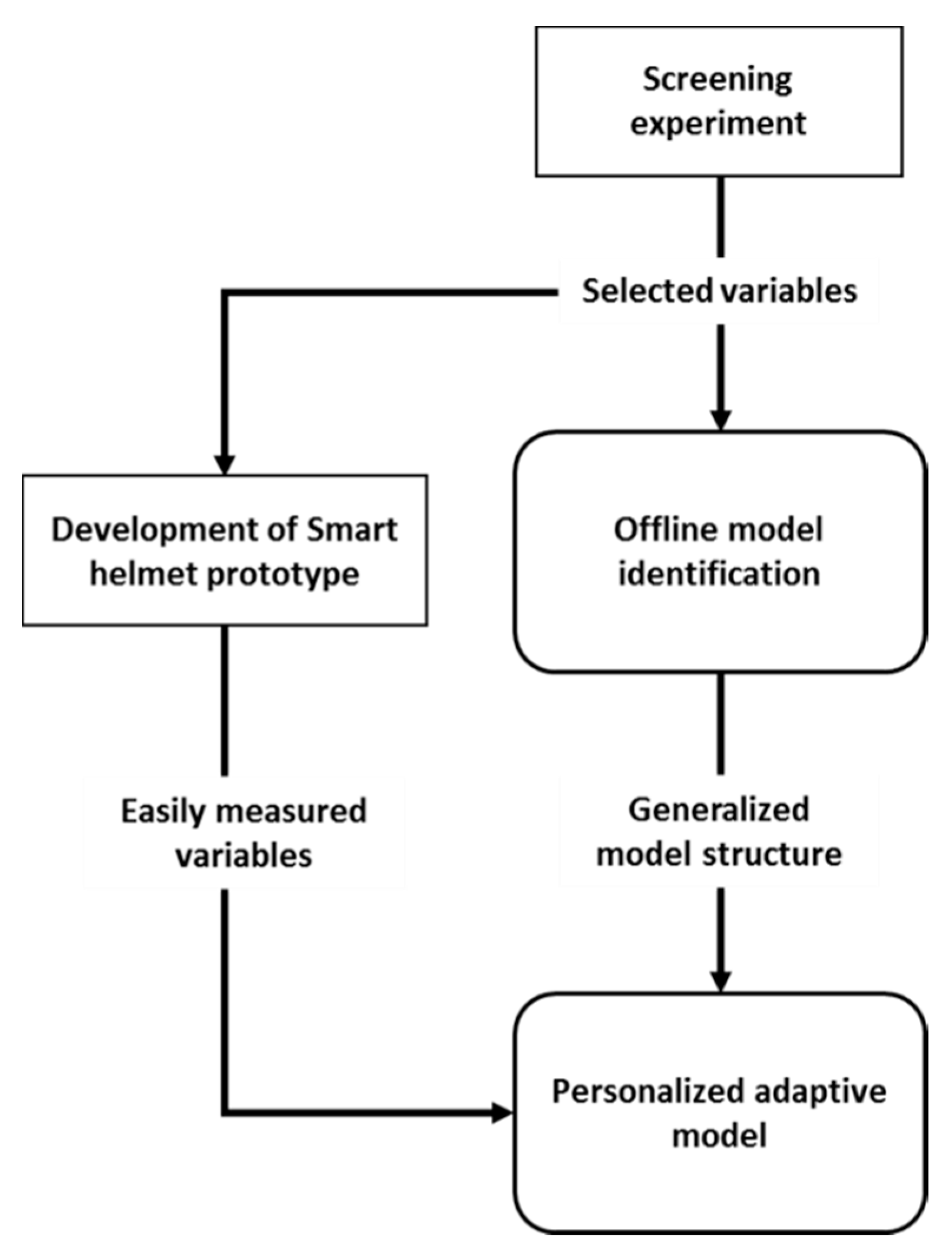
- (i)
- identifying a general model to estimate thermal comfort based on a few variables, the measurements of which can be integrated in helmets;
- (ii)
- developing and testing a prototype of a smart helmet based on the identified general thermal comfort model; and
- (iii)
- introducing the framework of calculation for an adaptive personalised reduced-order model to predict a cyclist’s under-helmet thermal comfort using nonintrusive, easily measured variables.
2. Materials and Methods
2.1. Development of General Thermal Comfort Predictive Model
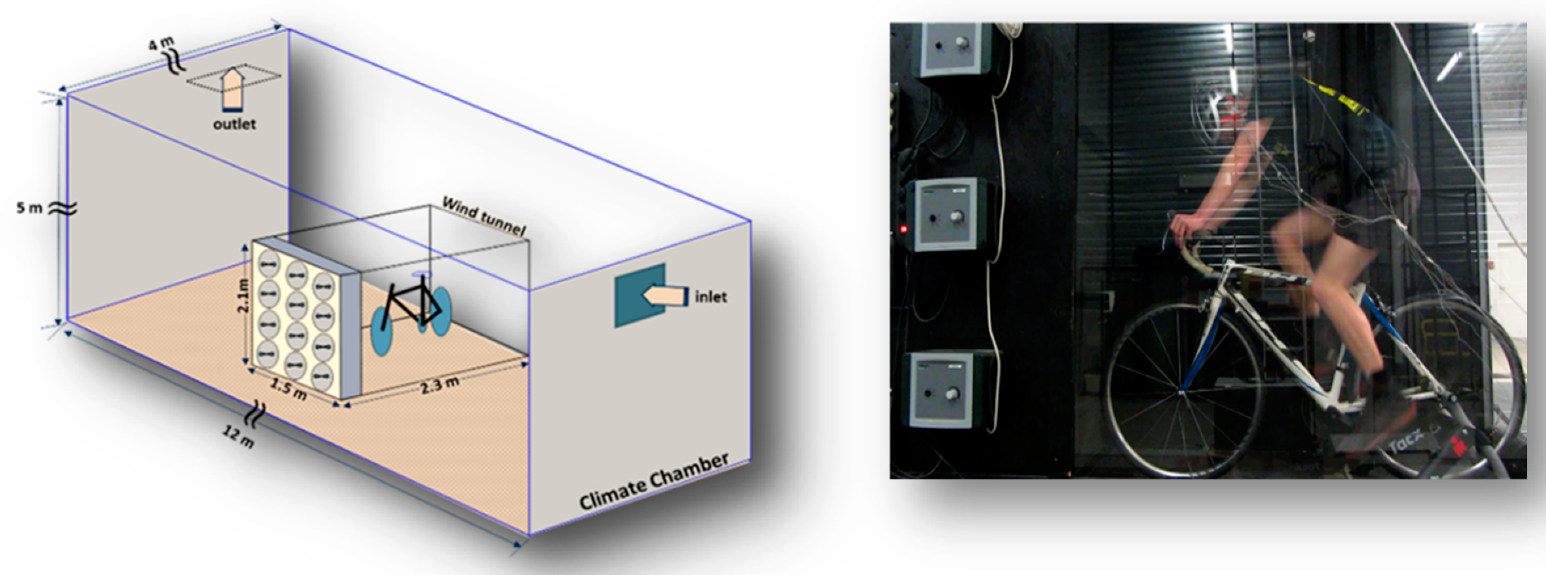
2.1.1. Experimental Setup and Test Subjects
2.1.2. Pretest Experiments
2.1.3. Thermal Comfort and Variable Screening Experimental Protocol
2.1.4. General Linear Regression (LR) Model Identification and Offline Parameter Estimation
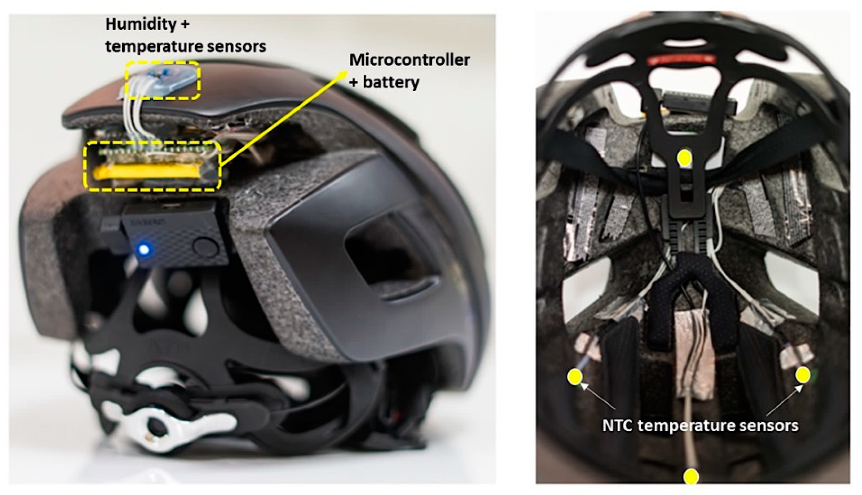
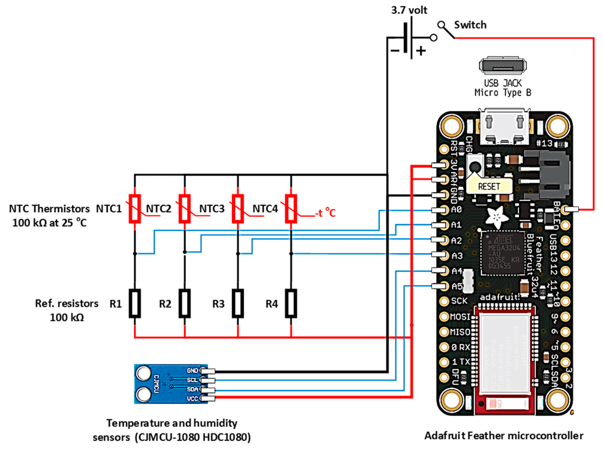
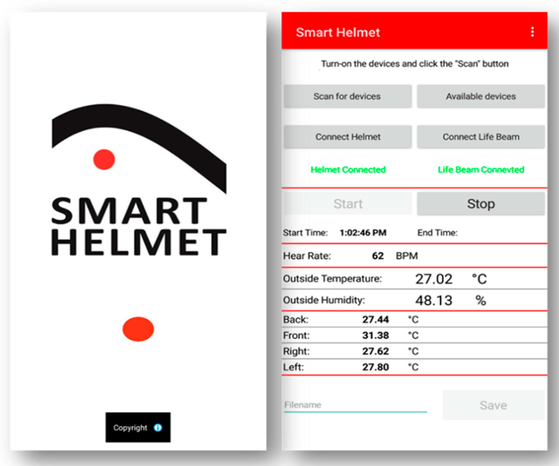
2.2. Development of Smart Helmet Prototype
2.3. Testing the Developed Smart Helmet Prototype
2.3.1. Test Subjects
2.3.2. Experimental Design and Protocol
3. Results
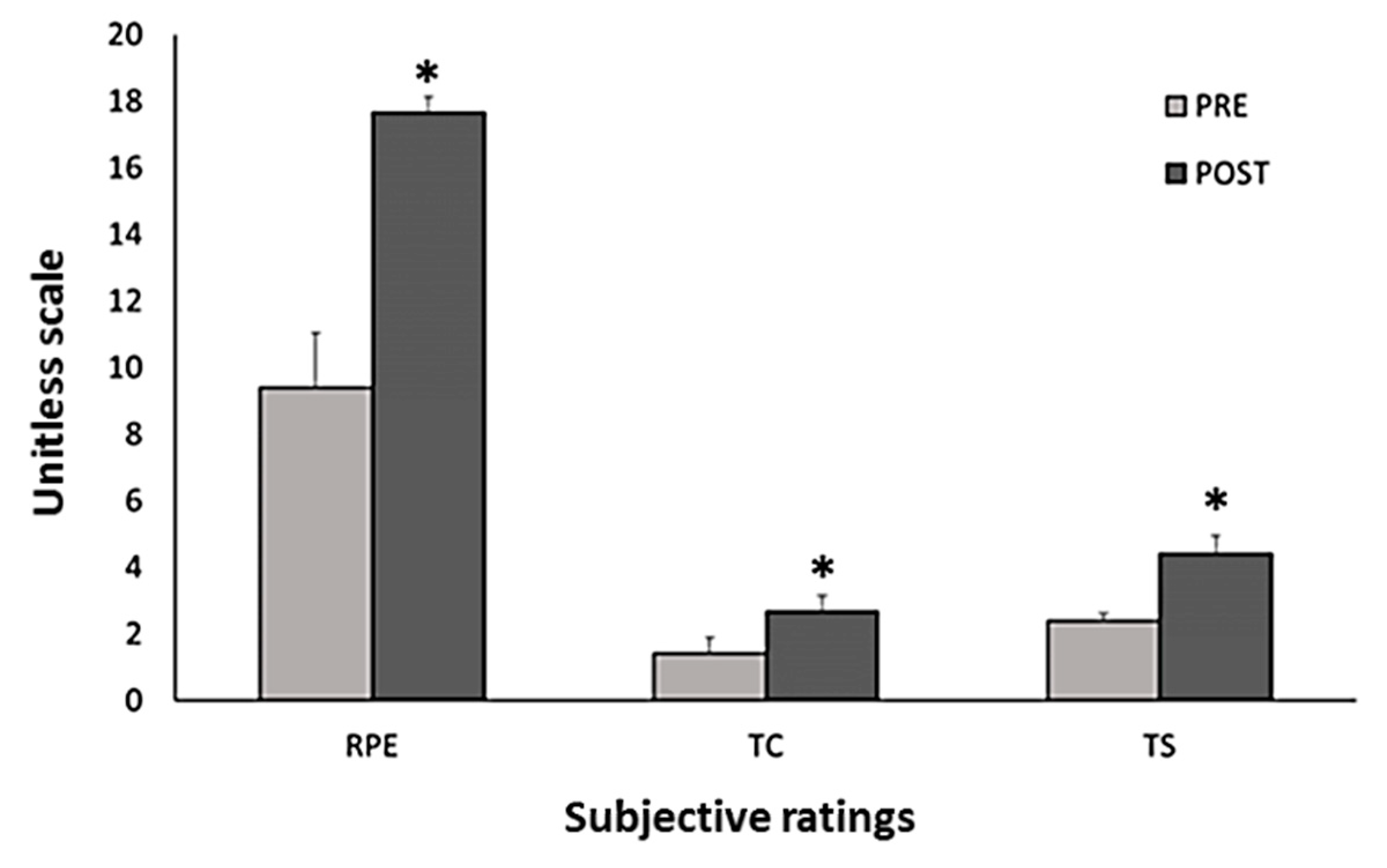
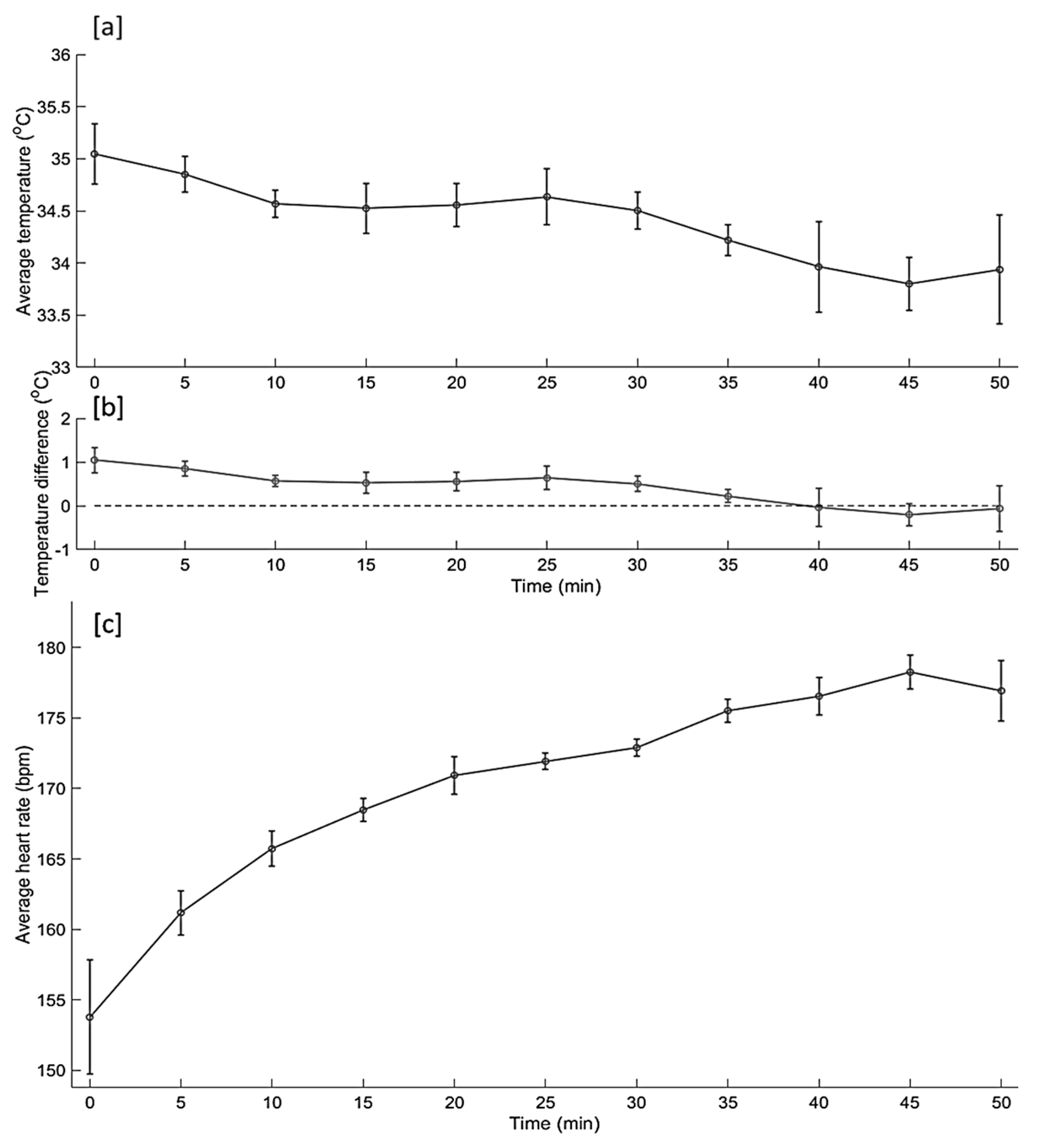
3.1. Pretest Experiments
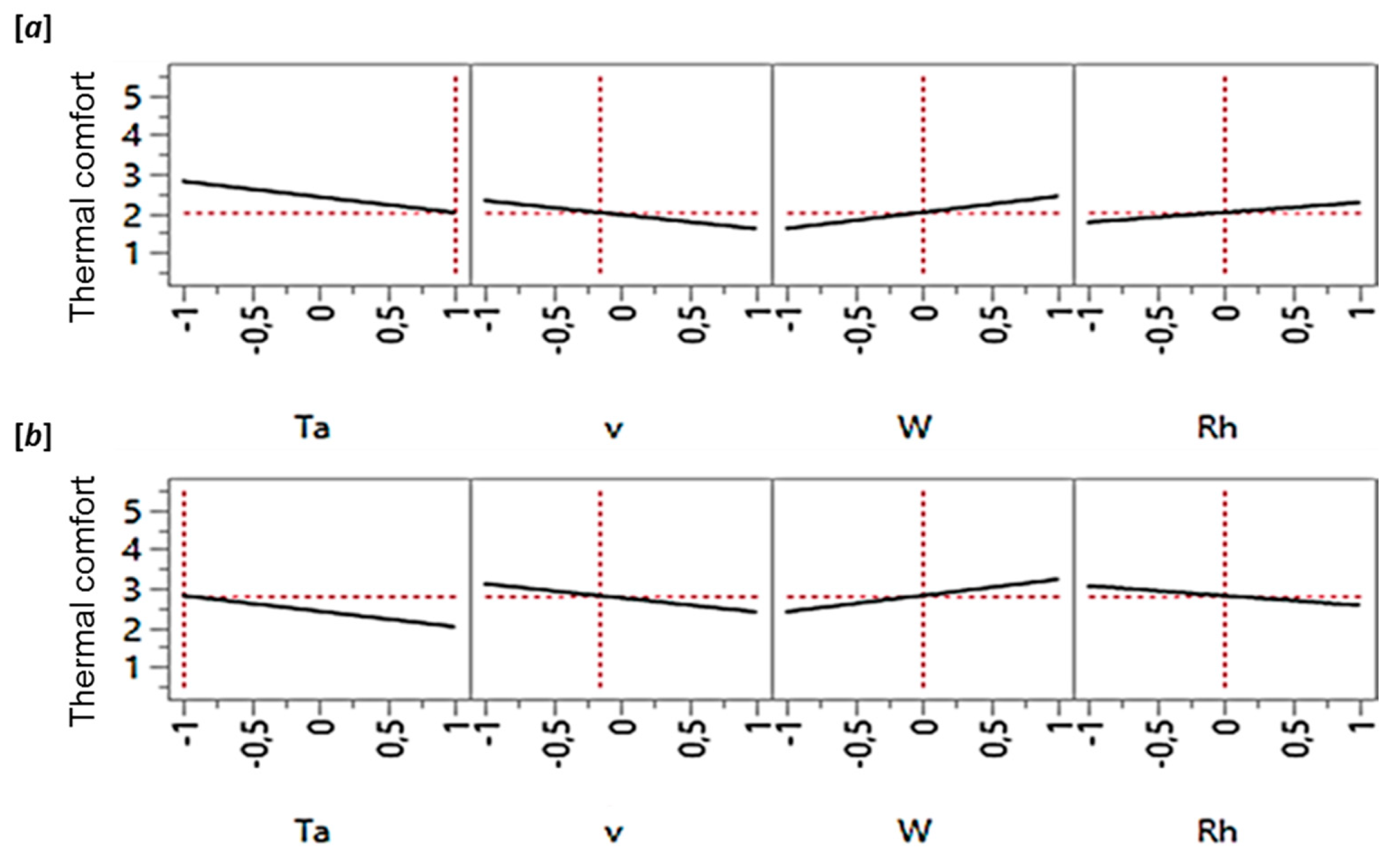
3.2. Development of Offline (General) Thermal Comfort Model
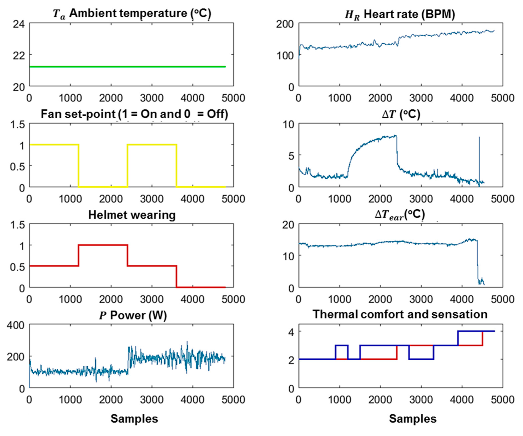
3.3. Testing the SmartHelmet Prototype and Validation of the Developed General Model
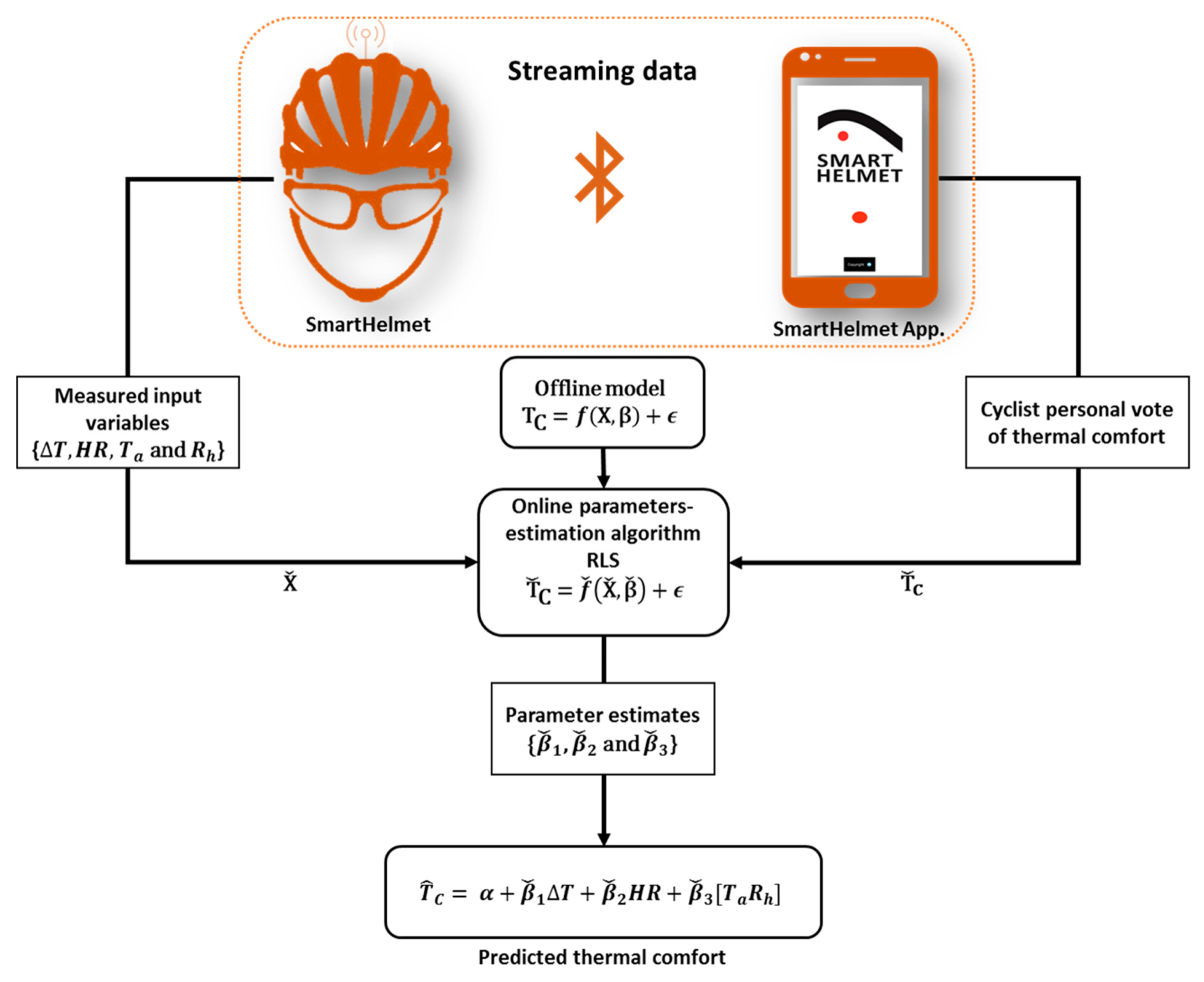
3.4. Introduction of Online Personalisation and Adaptive Modelling Algorithm
3.4.1. Offline Linear Regression Model
3.4.2. Streaming Data
3.4.3. Online Parameter Estimation Algorithm
4. Conclusions
Author Contributions
Funding
Acknowledgments
Conflicts of Interest
References
- Titze, S.; Bauman, A.; De Geus, B.; Krenn, P.; Kohlberger, T.; Reger-Nash, B.; Oja, P. Health benefits of cycling: A systematic review. Scand. J. Med. Sci. Sports 2011, 21, 496–509. [Google Scholar]
- Zentner, J.; Franken, H.; Löbbecke, G. Head injuries from bicycle accidents. Clin. Neurol. Neurosurg. 1996, 98, 281–285. [Google Scholar] [CrossRef]
- Elvik, R. Publication bias and time-trend bias in meta-analysis of bicycle helmet efficacy: A re-analysis of Attewell, Glase and McFadden, 2001. Accid. Anal. Prev. 2011, 43, 1245–1251. [Google Scholar] [CrossRef] [PubMed]
- Action, A.C.; Hope, T.U. Final Report of Working Group 2: Traffic Psychology; COST Action TU1101/HOPE: Brussels, Belgium, 2015. [Google Scholar]
- Finnoff, J.T.; Laskowski, E.R.; Altman, K.L.; Diehl, N.N. Barriers to Bicycle Helmet Use. Pediatrics 2001, 108, 2–10. [Google Scholar] [CrossRef] [PubMed]
- Bogerd, C.P.; Aerts, J.M.; Annaheim, S.; Bröde, P.; De Bruyne, G.; Flouris, A.D.; Kuklane, K.; Mayor, T.S.; Rossi, R.M. A review on ergonomics of headgear: Thermal effects. Int. J. Ind. Ergon. 2015, 45, 1–12. [Google Scholar] [CrossRef]
- Underwood, L.; Vircondelet, C.; Jermy, M. Thermal comfort and drag of a streamlined cycling helmet as a function of ventilation hole placement. Proc. Inst. Mech. Eng. Part P J. Sports Eng. Technol. 2018, 232, 15–21. [Google Scholar] [CrossRef]
- Mayor, T.S.; Couto, S.; Psikuta, A.; Rossi, R.M. Advanced modelling of the transport phenomena across horizontal clothing microclimates with natural convection. Int. J. Biometeorol. 2015, 59, 1875–1889. [Google Scholar] [CrossRef] [PubMed]
- ASHRAE. ASHRAE Standard 55; American Society of Heating, Refrigerating and Air-Conditioning Engineers, Inc.: Atlanta, GA, USA, 2017. [Google Scholar]
- Gagge, A.P.; Stolwijk, J.A.J.; Hardy, J.D. Comfort and thermal sensations and associated physiological responses at various ambient temperatures. Environ. Res. 1967, 1, 1–20. [Google Scholar] [CrossRef]
- Kenneth, C. Human Thermal Environments: The Effects of Hot, Moderate, and Cold Environments on Human Health, Comfort, and Performance, 3rd ed.; CRC Press: Boca Raton, FL, USA, 2014. [Google Scholar]
- Fanger, P.O. Thermal Comfort: Analysis and Applications in Environmental Engineering, 1st ed.; Danish Technical Press: Lyngby, Denmark, 1970. [Google Scholar]
- Enescu, D. Models and Indicators to Assess Thermal Sensation Under Steady-state and Transient Conditions. Energies 2019, 12, 841. [Google Scholar] [CrossRef]
- Koelblen, B.; Psikuta, A.; Bogdan, A.; Annaheim, S.; Rossi, R.M. Thermal sensation models: A systematic comparison. Indoor Air 2017, 27, 680–689. [Google Scholar] [CrossRef]
- Rugh, J.P.; Farrington, R.B.; Bharathan, D.; Vlahinos, A.; Burke, R.; Huizenga, C.; Zhang, H. Predicting human thermal comfort in a transient nonuniform thermal environment. Eur. J. Appl. Physiol. 2004, 92, 721–727. [Google Scholar] [CrossRef]
- Havenith, G.; Fiala, D. Thermal Indices and Thermophysiological Modeling for Heat Stress. Compr. Physiol. 2015, 6, 255–302. [Google Scholar]
- Youssef, A.; Truyen, P.; Brode, P.; Fiala, D.; Aerts, J.M. Towards Real-Time Model-Based Monitoring and Adoptive Controlling of Indoor Thermal Comfort. In Proceedings of the Ventilating Healthy Low-Energy Buildings, Nottingham, UK, 13–14 September 2017. [Google Scholar]
- De Bruyne, G.; Aerts, J.M.; Sloten, J.V.; Goffin, J.; Verpoest, I.; Berckmans, D. Quantification of local ventilation efficiency under bicycle helmets. Int. J. Ind. Ergon. 2012, 42, 278–286. [Google Scholar] [CrossRef]
- Gore, C.J. Physiological Tests for Elite Athletes Australian Sports Commmission; Human Kinetics: Champaign, IL, USA, 2000. [Google Scholar]
- Biochemistry, B.B.; Science, S. The Concept of Maximal Lactate Steady State. Sports Med. 2003, 33, 407–426. [Google Scholar]
- Beneke, R. Methodological aspects of maximal lactate steady state-implications for performance testing. Eur. J. Appl. Physiol. 2003, 89, 95–99. [Google Scholar] [CrossRef]
- Sibernagl, S. Atlas van de Fysiologie; SESAM/HBuitgevers: Baarn, The Netherlands, 2008. [Google Scholar]
- Fitts, R.H. Cellular mechanisms of muscle fatigue. Physiol. Rev. 1994, 74, 49–94. [Google Scholar] [CrossRef]
- Mukunthan, S.; Vleugels, J.; Huysmans, T.; de Bruyne, G. Latent Heat Loss of a Virtual Thermal Manikin for Evaluating the Thermal Performance of Bicycle Helmets. In Advances in Human Factors in Simulation and Modeling; Springer: Cham, Switzerland, 2019; pp. 66–78. [Google Scholar]
- Soong, T.T. Fundamentals of Probability and Statistics for Engineers; Wiley: Hoboken, NJ, USA, 2004. [Google Scholar]
- Borg, G.A. Psychophysical bases of perceived exertion. Med. Sci. Sports Exerc. 1982, 14, 377–381. [Google Scholar] [CrossRef]
- Box, G.E.P.; Draper, N.R. Empirical Model-Building and Response Surfaces; John Wiley & Sons: Oxford, UK, 1987. [Google Scholar]
- JMP® 14. JMP® 14 Profilers; Institute Inc.: Cary, NC, USA, 2018. [Google Scholar]
- Zinoubi, B.; Zbidi, S.; Vandewalle, H.; Chamari, K.; Driss, T. Relationships between rating of perceived exertion, heart rate and blood lactate during continuous and alternated-intensity cycling exercises. Biol. Sport 2018, 35, 29–37. [Google Scholar] [CrossRef]
- Takada, S.; Matsumoto, S.; Matsushita, T. Prediction of whole-body thermal sensation in the non-steady state based on skin temperature. Build. Environ. 2013, 68, 123–133. [Google Scholar] [CrossRef]
- Fiala, D. Dynamic Simulation of Human Heat Transfer and Thermal Comfort; De Montfort University: Leicester, UK, 1998. [Google Scholar]
- Lomas, K.J.; Fiala, D.; Stohrer, M. First principles modeling of thermal sensation responses in steady-state and transient conditions. ASHRAE Trans. 2003, 109, 179–186. [Google Scholar]
- Zhang, H. Human Thermal Sensation and Comfort in Transient and Non-Uniform Thermal Environments; University of California: Berkeley, CA, USA, 2003. [Google Scholar]
- Guan, Y.D.; Hosni, M.H.; Jones, B.W.; Gielda, T.P. Investigation of Human Thermal Comfort Under Highly Transient Conditions for Automotive Applications-Part 2: Thermal Sensation Modeling. ASHRAE Trans. 2003, 109, 898–907. [Google Scholar]
- Guan, Y.D.; Hosni, M.H.; Jones, B.W.; Gielda, T.P. Investigation of Human Thermal Comfort Under Highly Transient Conditions for Automotive Applications-Part 1: Experimental Design and Human Subject Testing Implementation. ASHRAE Trans. 2003, 109, 885–897. [Google Scholar]
- Nilsson, H.O.; Holmer, I. Comfort climate evaluation with thermal manikin methods and computer simulation models. Indoor Air 2003, 13, 28–37. [Google Scholar] [CrossRef]
- Kingma, B.R.M.; Schellen, L.; Frijns, A.J.H.; Lichtenbelt, W.D.V. Thermal sensation: A mathematical model based on neurophysiology. Indoor Air 2012, 22, 253–262. [Google Scholar] [CrossRef]
- Lu, S.; Wang, W.; Wang, S.; Hameen, E.C. Thermal Comfort-Based Personalized Models with Non-Intrusive Sensing Technique in Office Buildings. Appl. Sci. 2019, 9, 1768. [Google Scholar] [CrossRef]
- De Dear, R.; Brager, G.S. Developing an adaptive model of thermal comfort and preference. ASHRAE Trans. 1998, 104, 145–167. [Google Scholar]
- Kadlec, P.; Grbić, R.; Gabrys, B. Review of adaptation mechanisms for data-driven soft sensors. Comput. Chem. Eng. 2011, 35, 1–24. [Google Scholar] [CrossRef]
- Sharma, S.; Khare, S.; Huang, B. Robust online algorithm for adaptive linear regression parameter estimation and prediction. J. Chemom. 2016, 30, 308–323. [Google Scholar] [CrossRef]
- Zimmer, A.M.; Kurze, M.; Seidl, T. Adaptive Model Tree for Streaming Data. In Proceedings of the 2013 IEEE 13th International Conference on Data Mining, Dallas, TX, USA, 7–10 December 2013; pp. 1319–1324. [Google Scholar]
- Bouveyron, C.; Jacques, J. Adaptive linear models for regression: Improving prediction when population has changed. Pattern Recognit. Lett. 2010, 31, 2237–2247. [Google Scholar] [CrossRef][Green Version]
- Jiang, J.; Zhang, Y. A revisit to block and recursive least squares for parameter estimation. Comput. Electr. Eng. 2004, 30, 403–416. [Google Scholar] [CrossRef]
- Young, P.C. Recursive Estimation and Time-Series Analysis; Springer: Berlin, Germany, 2011. [Google Scholar]
- Benesty, J.; Paleologu, C.; Gänsler, T.; Ciochină, S. Recursive Least-Squares Algorithms; Springer: Berlin, Germany, 2011; pp. 63–69. [Google Scholar]
- Plackett, R.L. Some Theorems in Least Squares. Biometrika 1950, 37, 149. [Google Scholar] [CrossRef]
- Johnson, C.R. Lectures on Adaptive Parameter Estimation; Prentice-Hall: Upper Saddle River, NJ, USA, 1988. [Google Scholar]
- Vahidi, A.; Stefanopoulou, A.; Peng, H. Recursive least squares with forgetting for online estimation of vehicle mass and road grade: Theory and experiments. Veh. Syst. Dyn. 2005, 43, 31–55. [Google Scholar] [CrossRef]


| (°C) | (m·s−1) | (W) | (m2·°C·W−1) | |
|---|---|---|---|---|
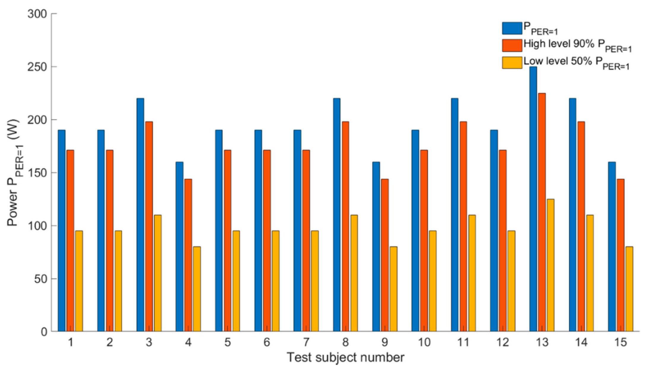
| Low level | 20 | 0 | 50% (PRER = 1) | 0 (no helmet) |
| Midlevel | / | / | / | 0.045 (with helmet) |
| High level | 30 | 4 | 90% (PRER = 1) | 0.060 (helmet + aeroshell) |
| Scale | Thermal Comfort Perception |
|---|---|
| 1 | Comfortable |
| 2 | Slightly uncomfortable |
| 3 | Uncomfortable |
| 4 | Very uncomfortable |
| Participant (No. = j) | Variables | Timeslot (1) | Timeslot (2) | Timeslot (3) | Timeslot (4) |
|---|---|---|---|---|---|
| = 1 | (°C) | ↓ | ↓ | ↓ | ↓ |
| (m·s−1) | ↑ | ↓ | ↑ | ↓ | |
| (% PPER = 1) | ↓ | ↓ | ↑ | ↑ | |
| (m2·°C·W−1) | − | ↑ | − | ↓ | |
| = 8 | (°C) | ↑ | ↑ | ↑ | ↑ |
| (m·s−1) | ↑ | ↑ | ↓ | ↓ | |
| (% PPER = 1) | ↑ | ↓ | ↑ | ↑ | |
| (m2·°C·W−1) | − | − | ↓ | ↑ |
| Variable | Average (±Standard Deviation) |
|---|---|
| Power output (W) | 176.5 (±24.2) |
| Cadence (rpm) | 93.7 (±14.2) |
| 30 km TT duration (min) | 56.9 (±7.9) |
| Term | Parameter | Estimate | Std. Error | t-Ratio | P > |t| |
|---|---|---|---|---|---|
| intercept | 2.36 | 0.14 | 16.80 | <0.0001 * | |
| −0.40 | 0.11 | −3.52 | 0.0025 * | ||
| −0.36 | 0.07 | −4.85 | <0.0001 * | ||
| 0.41 | 0.07 | 5.45 | <0.0001 * | ||
| 0.25 | 0.01 | 2.52 | 0.015 * |
| Term | Parameter | Estimate | Std. Error | t-Ratio | P > |t| |
|---|---|---|---|---|---|
| intercept | 1.86 | 0.21 | 13.61 | <0.0001 * | |
| 1.30 | 0.19 | 5.22 | 0.0031 * | ||
| −0.62 | 0.13 | −5.67 | <0.0014 * | ||
| 0.35 | 0.07 | 2.52 | 0.0140 * |
© 2019 by the authors. Licensee MDPI, Basel, Switzerland. This article is an open access article distributed under the terms and conditions of the Creative Commons Attribution (CC BY) license (http://creativecommons.org/licenses/by/4.0/).
Share and Cite
Youssef, A.; Colon, J.; Mantzios, K.; Gkiata, P.; Mayor, T.S.; Flouris, A.D.; De Bruyne, G.; Aerts, J.-M. Towards Model-Based Online Monitoring of Cyclist’s Head Thermal Comfort: Smart Helmet Concept and Prototype. Appl. Sci. 2019, 9, 3170. https://doi.org/10.3390/app9153170
Youssef A, Colon J, Mantzios K, Gkiata P, Mayor TS, Flouris AD, De Bruyne G, Aerts J-M. Towards Model-Based Online Monitoring of Cyclist’s Head Thermal Comfort: Smart Helmet Concept and Prototype. Applied Sciences. 2019; 9(15):3170. https://doi.org/10.3390/app9153170
Chicago/Turabian StyleYoussef, Ali, Jeroen Colon, Konstantinos Mantzios, Paraskevi Gkiata, Tiago S. Mayor, Andreas D. Flouris, Guido De Bruyne, and Jean-Marie Aerts. 2019. "Towards Model-Based Online Monitoring of Cyclist’s Head Thermal Comfort: Smart Helmet Concept and Prototype" Applied Sciences 9, no. 15: 3170. https://doi.org/10.3390/app9153170
APA StyleYoussef, A., Colon, J., Mantzios, K., Gkiata, P., Mayor, T. S., Flouris, A. D., De Bruyne, G., & Aerts, J.-M. (2019). Towards Model-Based Online Monitoring of Cyclist’s Head Thermal Comfort: Smart Helmet Concept and Prototype. Applied Sciences, 9(15), 3170. https://doi.org/10.3390/app9153170