A Survey of Handwritten Character Recognition with MNIST and EMNIST

1. Introduction

In recent years, deep learning-based techniques have been gaining significant interest in the research community for solving a variety of supervised, unsupervised and reinforcement learning problems. One of the most well-known and widely used techniques are convolutional neural networks (CNNs), a kind of neural networks which are able to automatically extract relevant features from input data.

The properties of convolutional neural networks, including the fact that they are able to retrieve features from multidimensional inputs, turn them into a very interesting alternative for solving problems within the field of computer vision. In fact, computer vision has become a testbed for validating novel techniques and innovations in CNNs.

More specifically, one dataset has been widely used for this purpose: the MNIST dataset. MNIST is a database of labeled handwritten digits, with separate training and test sets, and therefore is an easily interpretable domain that allows a fast comparison between different techniques. In fact, MNIST is so widely used that it is even used in “hello-world” tutorials of some deep learning frameworks, such as TensorFlow [1].

Soon after the release of the MNIST dataset in 1998, some authors have released rankings including the performance of different works. In fact, the first ranking was published by LeCun et al. [2], the authors of the original MNIST paper, and has included works as recent as 2012. To the best of our knowledge, the most recent and exhaustive ranking has been released by Benenson [3], updated as of 2016. However, this ranking is still very incomplete and omits a substantial number of relevant works, as well as those published after 2016. Finally, many authors of papers reporting results on the MNIST dataset have compared their performance against related works; however, they often include only other works using similar techniques.

As a consequence of this, there are not exhaustive and updated rankings of the MNIST database; and this paper intends to fill that gap. In particular, it gathers and summarizes all the works we have found reporting results on the MNIST dataset that are competitive; i.e., whose results are better than a 1% test error rate, classifying them according to two different criteria: whether they perform preprocessing and/or data augmentation or not, and whether the techniques used to obtain a given result involve convolutional neural networks or not. This paper has been written with completeness in mind, and therefore includes not only works published in journals and international conferences, but also those available in pre-print and source code repositories. However, results that are reported in works not published after a peer-review process are explicitly noted as so.

Additionally, as of today, MNIST is widely considered a non-challenging database anymore. As a consequence of it, an extended version of MNIST, namely EMNIST dataset was released in April 2017. EMIST comprises both handwritten digits and handwritten letters, is significantly larger than MNIST and data comes from a different source. In this paper, we also describe the acquisition of the EMNIST dataset and a survey of the state-of-the-art.

This paper is structured as follows: Section 2 describes the acquisition process for the MNIST database as well as the data format, and surveys the state of the art for the MNIST dataset. Then, Section 3 explains the acquisition process for the EMNIST database and the different subsets along with their format, later describing works using this dataset as well as NIST Special Database 19 (from which EMNIST is obtained). Finally, Section 4 summarizes the main findings found when surveying works on MNIST and EMNIST.

2. MNIST Database

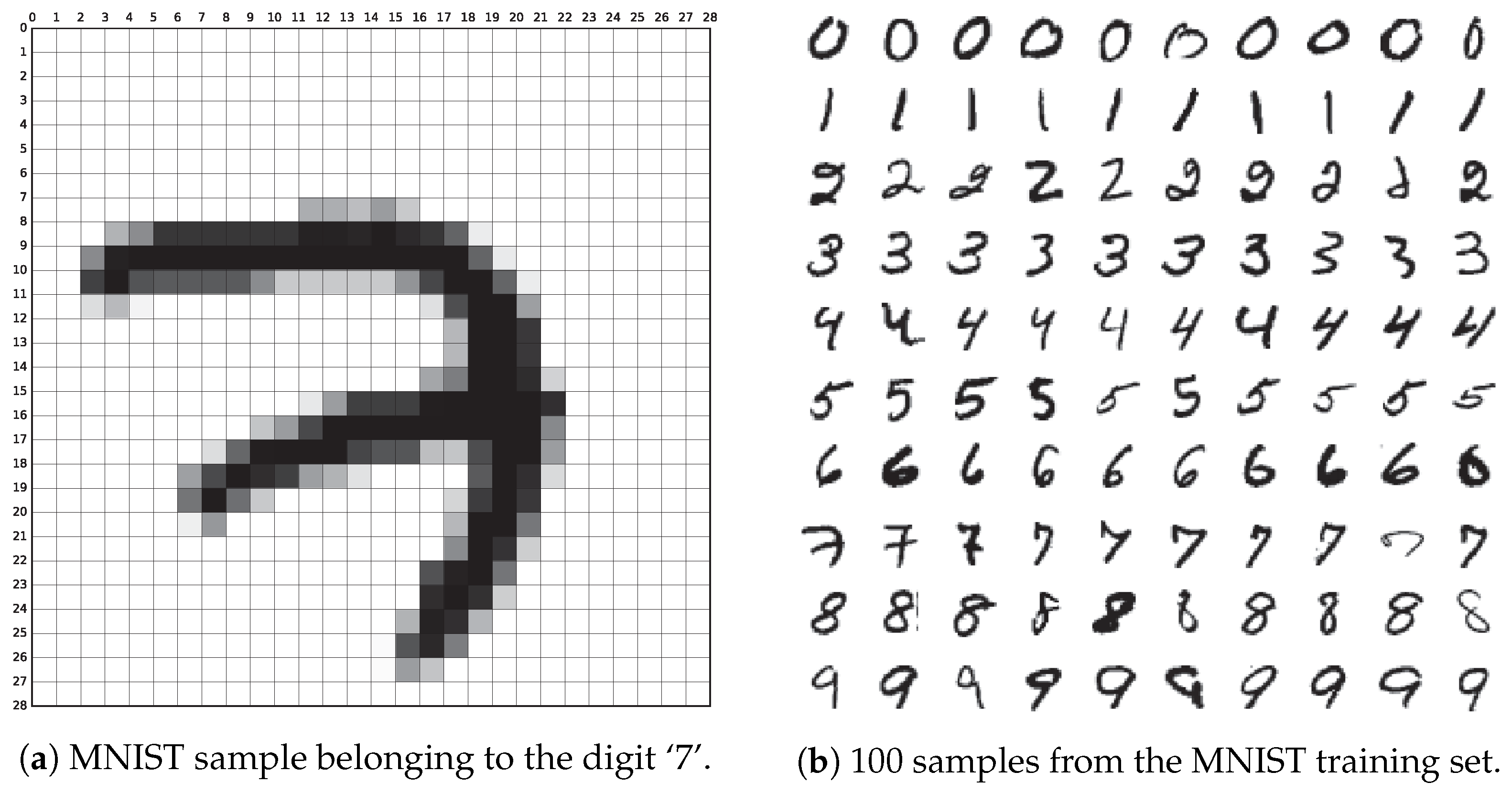
2.1. Acquisition and Data Format

The MNIST (Mixed National Institute of Standards and Technology) database was introduced by LeCun et al. [2] in 1998. Since then, this dataset has been widely used as a testbed for different machine learning and pattern recognition proposals.

The MNIST database contains a total of 70,000 instances, from which 60,000 are for training and the remainder are for testing. The database comprises two different sources: NIST’s Special Database 1 (collected among high-school students) and NIST’s Special Database 3 (retrieved from Census Bureau employees). The training and test set were chosen so that a same writer would not be involved in both sets. The training set contains samples from more than 250 writers.

Original images were submitted to preprocessing. This procedure first involved normalizing images to fit in a 20 × 20 pixel box while preserving the aspect ratio. Then, an anti-aliasing filter was applied, and as a result black and white images were effectively transformed into grayscale. Finally, blank padding was introduced to fit the images in a larger 28 × 28 pixel box, so that the center of mass of the digit matched its center. An example of a sample corresponding to the digit ‘7’ can be found in Figure 1a. A larger set of instances belonging to the training set is displayed in Figure 1b.

By looking at this figure, we can see that some digits can be easily confused. Depending on how they are written, it can be difficult to elucidate if a certain digit is a ‘4’ or a ‘9’, to say an example. Some cases of digits difficult to recognize, even for humans, can be seen in Figure 1b (see the ninth ‘2’ or the ninth ‘7’).

2.2. State of the Art

Because MNIST has been widely used to test the behavior of many implementations of classifiers, there has been an effort to publish some rankings in the past, using MNIST as a benchmark. Most of these rankings, as well as the established literature uses the “test error rate” metric when referring to performance over MNIST. This metric is the percentage of incorrectly classified instances.

One of the earliest rankings was published by LeCun et al. [2] themselves, which includes references up to 2012. This website provides a taxonomy of classifiers and points out whether each work performed data preprocessing or augmentation (addition of new instances to the training set resulting from distortions or other modifications of the original data).

In this ranking, we can verify that the early machine learning approaches used by LeCun et al. [4] included linear classifiers (whose error rate ranges from 7.6 to 12%), K-nearest neighbors approaches (K-NN, ranging from 1.1 to 5%), non-linear classifiers (about 3.5%), support vector machines (SVM, from 0.8 to 1.4%), neural networks (NN, from 1.6 to 4.7%) and convolutional neural networks (CNN, from 0.7 to 1.7%). It is remarkable that data augmentation leads to better results, in particular, the best error rate achieved using a convolutional neural network with no distortions and no preprocessing in LeCun et al. [4] was 0.95%.

From the different works gathered in LeCun et al.’s ranking, those based in convolutional neural networks outperform the other techniques. However, there are some classical machine learning techniques which are still able to provide competitive error rates (in this paper, we will consider “competitive” those techniques achieving an error rate under 1.0%). For instance, Belongie et al. [5] achieved 0.63% and Keysers et al. [6] achieved 0.54% and 0.52% using K-NN, Kégl and Busa-Fekete [7] achieved 0.87% using boosted stumps on Haar features, LeCun et al. [4] achieved 0.8% and Decoste and Schölkopf [8] attained results from 0.56 to 0.68% using SVM.

When using non-convolutional neural networks, Simard et al. [9] achieved 0.9% and 0.7% respectively using a 2-layer neural network with MSE and cross-entropy loss functions. Deng and Yu [10] achieved 0.83% using a deep convex network without data augmentation or preprocessing. Very interesting results were attained by Meier et al. [11] (0.39%) using a committee of 25 neural networks and Cireşan et al. [12] (0.35%) using a 6-layers neural network (it is worth mentioning that the reproducibility of this result has been put into question by Martin [13] in his blog).

On the other hand, works based on convolutional neural networks attained a much better average performance (in fact, the worst result reported in LeCun’s ranking was 1.7%). LeCun et al. [4] combined different convolutional architectures along with data augmentation techniques, obtaining error rates ranging from 0.7 to 0.95%. Lauer et al. [14] attained between 0.54% and 0.83% using a trainable feature extractor along with SVMs, and Labusch et al. [15] reported an error rate of 0.59% using a similar technique consisting on a CNN to extract sparse features and SVMs for classification. Simard et al. [9] obtained error rates between 0.4% and 0.6% using CNN with cross-entropy loss function and data augmentation. Ranzato et al. [16] reported results between 0.39% and 0.6% using a large CNN along with unsupervised pretraining, and some years later Jarrett et al. [17] reported a test error of 0.59% with a similar approach technique and without data augmentation. The best results in this ranking are those obtained by Cireşan et al. [18], which reported an error rate of 0.35% using a large CNN, and 0.27% [19] and 0.23% [20] using committees of 7 and 35 neural networks respectively, using data augmentation in all cases.

In 2015, McDonnell et al. [21] proposed an approach using the ‘extreme learning machine’ (ELM) [22] algorithm to train shallow non-convolutional neural networks, and they agree on the fact that data augmentation with distortions can reduce error rates even further. In their work, McDonnell et al. compare their results with other previous ELM and selected non-ELM approaches, updated with some CNN-based works as of 2015. The most outstanding ELM-based results achieved test error rates of 0.97% in the work by Kasun et al. [23], and ranged from 0.57 to 1.36% in the proposal by McDonnell et al. [21].

However, most interesting results included in the comparison by McDonnell et al. [21] are not those provided in that work, but those from previous works where convolutional neural networks were used. For example, Wan et al. [24] used CNNs with a generalization of dropout they called DropConnect, and reported an error rate of 0.57% without data augmentation and as low as 0.21% with data augmentation. Zeiler and Fergus [25] proposed the use of stochastic pooling achieving an error rate of 0.47%. Goodfellow et al. [26] described the maxout model averaging technique, attaining a test error rate of 0.45% without data augmentation. In 2015, Lee et al. [27] described “deeply supervised nets”, an approach by which they introduce a classifier (SVM or softmax) at hidden layers, reporting a result of 0.39% without data augmentation.

A more recent ranking, updated as of 2016, has been made available by Benenson [3] in his GitHub’s page. This ranking includes many of the works reviewed so far, as well as other with very competitive results. For example, Sato et al. [28] explore and optimize data augmentation, and attain a test error rate of 0.23% in the MNIST database using a convolutional neural network. A very interesting result is reported by Chang and Chen [29], where an error rate of 0.24% (the best result found as of 2017 in the state of the art without data augmentation) was obtained by using a network-in-network approach with a maxout multi-layer perceptron, an approach they named MIN. Also, very competitive performances without data augmentation were reported by Lee et al. [30] when using gated pooling functions in CNNs (0.29%), by Liang and Hu [31] when using a recurrent CNN (0.31%), by Liao and Carneiro [32] when using CNNs with normalization layers and piecewise linear activation units (0.31%) and competitive multi-scale convolutional filters (0.33%) [33], or by Graham Graham [34] using fractional max-pooling with random overlapping (0.32%).

Additional works where state-of-the-art results were obtained without data augmentation include those by McFonnell and Vladusich [35], who reported a test error rate of 0.37% using a fast-learning shallow convolutional neural network, Mairal et al. [36], who achieved 0.39% using convolutional kernel networks, Xu et al. [37], who explored multi-loss regularization in CNNs obtaining an error rate of 0.42%, and Srivastava et al. [38] used so-called convolutional “highway" networks (inspired by LSTM recurrent networks) to achieve an error rate of 0.45%.

Lin et al. [39] reported an error rate of 0.47% using a network-in-network approach, where micro-neural networks are used as convolutional layers. Ranzato et al. [40] used convolutional layers for feature extraction and two fully connected NN for classification, attaining an error rate of 0.62%. Bruna and Mallat [41] designed a network that performed wavelet transform convolutions to the input and a generative PCA (principal component analysis) classifier to obtain an error of 0.43%.

Calderón et al. [42] proposed a variation of a CNN where the first layer applies Gabor filters over the input, obtaining an error of 0.68%. Also, Le et al. [43] explored the application of limited-memory BFGS (L-BFGS) and conjugate gradient (CG) as alternatives to stochastic gradient descent methods for network optimization, achieving 0.69% error rate. Finally, Yang et al. [44] developed a new transform named Adaptative Fastfood to reparameterize the fully connected layers, obtaining a test error rate of 0.71%.

An interesting approach is followed by Hertel et al. [45], in which they reuse the convolutional kernels previously learned over the ILSVRC-12 dataset, proving that CNNs can learn generic feature extractors than can be reused across tasks, and achieving a test error rate in the MNIST dataset of 0.46% (vs. 0.32% when training the network from scratch).

It can be seen how most recent works are based on convolutional neural networks, due to their high performance. However, some exceptions can be noticed. One example is the work by Wang and Tan [46] where they attained a test error rate of 0.35% using a single layer centering support vector data description (C-SVDD) network with multi-scale receptive voting and SIFT (scale-invariant feature transform) features. Also, Zhang et al. [47] devised a model (HOPE) for projecting features from raw data, that could be used for training a neural network, that attained a test error rate of 0.40% without data augmentation. Visin et al. [48] proposed a recurrent neural network (RNN) that replaced the convolutional layers by recurrent neural networks that swiped through the image, attaining an error rate of 0.45% with data augmentation.

Additional examples with less performance include the work by Azzopardi and Petkov [49] who used a combination of shifted filter responses (COSFIRE), attaining an error rate of 0.52%. Also, Chan et al. Chan et al. [50] used a PCA network to learn multi-stage filter banks, and report an error rate of 0.62%. Mairal et al. [51] used task-driven dictionary learning, reporting a test error rate of 0.54%, yet using data augmentation. Jia et al. [52] explored the receptive field of pooling, and obtained an error of 0.64%. Thom and Palm [53] explored the application of the sparse connectivity and sparse activity properties to neural networks, obtaining an error rate of 0.75% using a supervised online autoencoder with data augmentation. Lee et al. [54] described convolutional deep belief networks with probabilistic max-pooling achieving an error rate of 0.82%. Min et al. [55] reported an error of 0.95% using a deep encoder network to perform non-linear feature transformations which are then introduced to K-NN for classification. Finally, Yang et al. [56] used supervised translation-invariant sparse coding with a linear SVM attaining an error rate of 0.84%.

Other approach to solve the MNIST classification problem involves so-called “deep Boltzmann machines”. The first application of this technique was suggested by Salakhutdinov and Hinton [57] and enabled them to report an error rate of 0.95%. Few years later, Goodfellow et al. [58] introduced the multi-prediction deep Boltzmann machine, achieving a test error rate of 0.88%.

The reviewed rankings gather most of the works providing very competitive results for the MNIST database. Besides those rankings, we have found a work by Mishkin and Matas [59] where the authors work in the weights initialization of the CNN and replacing the softmax classifier with SVM, achieving a test error rate of 0.38%, and another work by Alom et al. [60] where inception-recurrent CNNs were used to attain an error of 0.29%.

Finally, it is worth mentioning some techniques that automatically optimize the topology of CNNS: MetaQNN [61], which relies on reinforcement learning for the design of CNNs architectures, has reported an error rate on MNIST of 0.44%, and 0.32% when using an ensemble of the best found neural networks. Also, DEvol [62], which uses genetic programming, has obtained a error rate of 0.6%. Baldominos et al. [63] presented a work in 2018 where the topology of the network is evolved using grammatical evolution, attaining a test error rate of 0.37% without data augmentation and this result was later improved by means of the neuroevolution of committees of CNNs [64] down to 0.28%. Similar approaches of evolving a committee of CNNs were presented by Bochinski et al. [65], achieving a very competitive test error rate of 0.24%; and by Baldominos et al. [66], where the models comprising the committee were evolved using a genetic algorithm, reporting a test error rate of 0.25%.

A summary of all the reviewed works can be found in

Table 1. Side-by-side comparison of the most competitive (error rate < 1%) results found in the state of the art for the MNIST database with data augmentation or preprocessing. Best achieved performances are boldfaced.

Technique	Test Error Rate
NN 6-layer 5,700 hidden units [12]	0.35%
MSRV C-SVDDNet [46]	0.35%
Committee of 25 NN 2-layer 800 hidden units [11]	0.39%
RNN [48]	0.45%
K-NN (P2DHMDM) [6]	0.52%
COSFIRE [49]	0.52%
K-NN (IDM) [6]	0.54%
Task-driven dictionary learning [51]	0.54%
Virtual SVM, deg-9 poly, 2-pixel jit [8]	0.56%
RF-C-ELM, 15,000 hidden units [21]	0.57%
PCANet (LDANet-2) [50]	0.62%
K-NN (shape context) [5]	0.63%
Pooling + SVM [52]	0.64%
Virtual SVM, deg-9 poly, 1-pixel jit [8]	0.68%
NN 2-layer 800 hidden units, XE loss [9]	0.70%
SOAE-$\sigma$ with sparse connectivity and activity [53]	0.75%
SVM, deg-9 poly [4]	0.80%
Product of stumps on Haar f. [7]	0.87%
NN 2-layer 800 hidden units, MSE loss [9]	0.90%
CNN (2 conv, 1 dense, relu) with DropConnect [24]	0.21%
Committee of 25 CNNs [20]	0.23%
CNN with APAC [28]	0.23%
CNN (2 conv, 1 relu, relu) with dropout [24]	0.27%
Committee of 7 CNNs [19]	0.27%
Deep CNN [18]	0.35%
CNN (2 conv, 1 dense), unsup pretraining [16]	0.39%
CNN, XE loss [9]	0.40%
Scattering convolution networks + SVM [41]	0.43%
Feature Extractor + SVM [14]	0.54%
CNN Boosted LeNet-4 [4]	0.70%
CNN LeNet-5 [4]	0.80%

and

Table 2. Side-by-side comparison of the most competitive (error rate < 1%) results found in the state of the art for the MNIST database without data augmentation or preprocessing. Best achieved performances are boldfaced.

Technique	Test Error Rate
HOPE+DNN with unsupervised learning features [47]	0.40%
Deep convex net [10]	0.83%
CDBN [54]	0.82%
S-SC + linear SVM [56]	0.84%
2-layer MP-DBM [58]	0.88%
DNet-kNN [55]	0.94%
2-layer Boltzmann machine [57]	0.95%
Batch-normalized maxout network-in-network [29]	0.24%
Committees of evolved CNNs (CEA-CNN) [65]	0.24%
Genetically evolved committee of CNNs [66]	0.25%
Committees of 7 neuroevolved CNNs [64]	0.28%
CNN with gated pooling function [30]	0.29%
Inception-Recurrent CNN + LSUV + EVE [60]	0.29%
Recurrent CNN [31]	0.31%
CNN with norm. layers and piecewise linear activation units [32]	0.31%
CNN (5 conv, 3 dense) with full training [45]	0.32%
MetaQNN (ensemble) [61]	0.32%
Fractional max-pooling CNN with random overlapping [34]	0.32%
CNN with competitive multi-scale conv. filters [33]	0.33%
CNN neuroevolved with GE [63]	0.37%
Fast-learning shallow CNN [35]	0.37%
CNN FitNet with LSUV initialization and SVM [59]	0.38%
Deeply supervised CNN [27]	0.39%
Convolutional kernel networks [36]	0.39%
CNN with Multi-loss regularization [37]	0.42%
MetaQNN [61]	0.44%
CNN (3 conv maxout, 1 dense) with dropout [17]	0.45%
Convolutional highway networks [38]	0.45%
CNN (5 conv, 3 dense) with retraining [45]	0.46%
Network-in-network [39]	0.47%
CNN (3 conv, 1 dense), stochastic pooling [25]	0.49%
CNN (2 conv, 1 dense, relu) with dropout [24]	0.52%
CNN, unsup pretraining [17]	0.53%
CNN (2 conv, 1 dense, relu) with DropConnect [24]	0.57%
SparseNet + SVM [15]	0.59%
CNN (2 conv, 1 dense), unsup pretraining [16]	0.60%
DEvol [62]	0.60%
CNN (2 conv, 2 dense) [40]	0.62%
Boosted Gabor CNN [42]	0.68%
CNN (2 conv, 1 dense) with L-BFGS [43]	0.69%
Fastfood 1024/2048 CNN [44]	0.71%
Feature Extractor + SVM [14]	0.83%
Dual-hidden Layer Feedforward Network [21]	0.87%
CNN LeNet-5 [4]	0.95%

. Table 1 includes works where some preprocessing or data augmentation took place before classification, whereas Table 2 includes the remaining works. The top of the table shows the performance of classical machine learning, while the lower side shows the results reported using CNNs. In those cases when authors have reported more than one result using a single classifier (e.g., with different parameters), only the best is shown.

3. EMNIST Database

3.1. Acquisition and Data Format

As it can be observed from the previous section, there are a significant amount of works tested over MNIST and reporting a test error rate of 1%. The fact that many of these works approach an error rate of 0.2% suggests that this value can be irreducible for this problem. For this reason, MNIST is considered to be already solved. As a result, Cohen et al. [67] introduced in April 2017 the Extended MNIST database (EMNIST), consisting on both handwritten digits and letters, and sharing the same structure than the MNIST database. Authors of EMNIST stated that at that point “the dataset labeling can be called into question”, describing MNIST as a non-challenging benchmark.

A sample of the letters and digits in the EMNIST dataset can be found in Figure 2.

The source for building EMNIST database was NIST Special Database 19 (NIST SD 19) [68], containing NIST’s (National Institute of Standards and Technology of the US) entire corpus of training materials for handprinted document and character recognition, including over 800,000 manually checked and labelled characters from almost 3700 writers [69] who filled a form. Even if this database was available from the mid-1990s, it remained mostly unused due to the difficulty in accessing and using it in modern computers, because of the way it was stored. This was fixed in 2016 when a second version of the database was released with a simpler format.

The authors of EMNIST have intentionally made the database compliant with MNIST in terms of structure, therefore performing a similar processing, which involves the following steps:

• Storing original images in NIST SD 19 as 128 × 128-pixels black and white images.
• Applying a Gaussian blur filter to soften edges.
• Removing empty padding to reduce the image to the region of interest.
• Centering the digit in a square box preserving the aspect ration.
• Adding a blank padding of 2-pixels per side.
• Downsampling the image 28 × 28 pixels using bi-cubic interpolation.

Originally, NIST SD 19 had two different labeling schemata:

• By_Class: in this schema classes are digits [0–9], lowercase letters [a–z] and uppercase letters [A–Z]. Thus, there are 62 different classes.
• By_Merge: this schema addresses the fact that some letters are quite similar in their lowercase and uppercase variants, thus both classes can be fused. In particular, these letter are ‘c’, ‘i’, ‘j’, ‘k’, ‘l’, ‘m’, ‘o’, ‘p’, ‘s’, ‘u’, ‘v’, ‘w’, ‘x’, ‘y’ and ‘z’. This schema contains 47 classes.

These schemata have been ported to EMNIST. Also, besides these two datasets, EMNIST has generated additional datasets:

• Balanced: both By_Class and By_Merge datasets are very unbalanced when it comes to letters, a fact that could negatively impact the classification performance. This dataset takes the By_Merge dataset and reduces the number of instances from 814,255 (total number of samples in NIST Special Database 19) to only 131,600, guaranteeing that there is an equal number of samples per each label.
• Digits: similar to MNIST, but from a different source and with 280,000 instances.
• Letters: this dataset contains mixed lowercase and uppercase letteres, thus containing 26 classes and a total of 145,600 samples.

3.2. State of the Art

In the original EMNIST paper [67], authors included a baseline using a linear classifier and another technique named OPIUM (Online Pseudo-Inverse Update Method), a classifier introduced by van Schaik and Tapson [70]. Authors declared to have chosen this technique because it generates an analytical solution which is deterministic, and their aim was not to obtain cutting-edge results. In fact, they report an accuracy of 85.15% in the Letters dataset and 95.90% in the Digits dataset using OPIUM. Since Cohen et al. [67] reported the performance in terms of accuracy instead of error rate, we have decided to do so as well in this survey.

Techniques not belonging to the field of deep learning have been tested on EMNIST with successful results. For example, Ghadekar et al. [71] discrete wavelet transform (DWT) and discrete cosine transform (DCT) were hybridized to extract features from the handwritten samples, later using K-NN and SVM for classification. Authors report that SVM outperform K-NN in all scenarios, attaining an accuracy of up to 89.51% in EMNIST Letters and 97.74% in EMNIST Digits.

As it happened with MNIST, outstanding achievements have been possible in EMNIST when testing deep learning techniques. This can be seen in a recent paper by Botalb et al. [72] comparing a multi-layer perceptron with CNNs in EMNIST. They report a maximum accuracy of 89.47% using a multi-layer perceptron, and an accuracy of 99.2% using a CNN, although the test set used by authors is not standard. An early attempt to use deep learning to EMNIST was presented by Peng and Yin [73], who described the application of Markov random field-based CNNs reporting accuracies ranging between 87.77% and 99.75%. Singh et al. [74] have used a CNN with three convolutional layers and two dense layers, reporting an accuracy in EMNIST Digits of 99.62%. Mor et al. [75] used a CNN with two convolutional layers and one dense layer for classifying EMNIST with the purpose of developing a handwritten text classification app for Android, obtaining an accuracy of 87.1% over EMNIST By_Class.

An interesting work using capsule layers (a concept recently introduced by Sabour et al. [76]) is TextCaps [77], a CNN with 3 convolutional layers and two capsule layers, which obtain accuracies of 95.36% in EMNIST Letters and 99.79% in EMNIST Digits. Another interesting work was published by dos Santos et al. [78], where they proposed the use of deep convolutional extreme learning machine, where gradient descent is not used to train the network, allowing a very fast learning stage (only 21 min using CPU, according to authors). They tested their proposal only with EMNIST Digits, attaining an accuracy of 99.775%. Finally, Cavalin and Oliveira [79] presented a method to generate a hierarchical classifier by automatically studying the confusion matrix of a “flat” (regular) classifier. They test logistic regression, multi-layer perceptrons and CNNs, and report the best results for the CNN, although with this technique the hierarchical classification do not beat the flat setting. They report an accuracy of 99.46% for EMNIST Digits and 93.63% for EMNIST Letters.

Recently, some authors have made used of neural architecture search for automatically optimizing the hyperparameters of CNN classifiers. For example, Dufourq and Bassett [80] presented EDEN, where they applied neuroevolution obtaining an accuracy of 88.3% in EMNIST Balanced and 99.3% in EMNIST Digits. More recently, [64] have used committees of neuroevolved CNNs using topology transfer learning, obtaining an accuracy of 95.35% in EMNIST Letters and 99.77% in EMNIST Digits.

EMNIST database has been used in some application papers as well. As an example, the dataset has also been used by Neftci et al. [81] for training neuromorphic deep neural networks and by Shu et al. [82] for the sake of pairwise classification. However, due to the way in which the dataset was used, results are not comparable other works. Srivastava et al. [83] used EMNIST for training a optical character recognition system for bank cheques, and Sharma et al. [84] used the database for optical recognition in specialized forms filled by students, although in neither case performance on the EMNIST test set was reported. Similarly, Shawon et al. [85] designed a system using a CNN with six convolutional layers and two fully connected layers for Bangla handwritten digit recognition, testing it also in EMNIST and reporting accuracies of 90.59% in EMNIST Balanced and 99.79% in EMNIST Digits.

Additionally, some researchers have relied on NIST SD 19 in the past as a testbed for their proposals. These works are not directly comparable to EMNIST since datasets are not identical, but can be used as a reference. For example, Milgram et al. [86] reported an average accuracy of 98.75% using SVMs with sigmoid function over a test set made only of digits. Granger et al. [87] used particle swarm optimization for evolving the topology of neural networks, obtaining an accuracy over a test set of digits of 96.49%. Moreover, Oliveira et al. [88] tested a multi-layer perceptron, reporting an accuracy of 98.39% in the same dataset.

In other works, letters from NIST SD 19 are also taken into account. For example, Radtke et al. [89] optimized a classifier using an annealing-based approach called record-to-record travel reporting an accuracy of 93.78% for letters and 96.53% for digits. Koerich and Kalva [90] tested a multi-layer perceptron attaining an accuracy of 87.79% in the letters dataset. Also, Cavalin et al. [91] used hidden Markov models reporting an accuracy of 87% for letters (both uppercase and lowercase) and 98% for digits. Finally, Cireşan et al. [19] have used this database to test the performance of committees of CNNs, attaining accuracies of 88.12% for the whole database, 92.42% for letters and 99.19% for digits.

Surveyed works are summarized in

Table 3. Side-by-side comparison of the results for the EMNIST dataset, including works using similar datasets from NIST Special Database 19. Best results are boldfaced. Results marked with a star (*) indicate that they refer to works using samples from NIST SD 19 which are similar but not equivalent to EMNIST (samples are the same, but they are not submitted to the preprocessing stage used in EMNIST, described in the text).

Technique	By_Class	By_Merge	Balanced	Letters	Digits
DWT-DCT + SVM [71]	–	–	–	89.51%	97.74%
Linear classifier [67]	51.80%	50.51%	50.93%	55.78%	84.70%
OPIUM [67]	69.71%	72.57%	78.02%	85.15%	95.90%
SVMs (one against all + sigmoid) [86]	–	–	–	–	98.75% *
Multi-layer perceptron [88]	–	–	–	–	98.39% *
Hidden Markov model [91]	–	–	–	90.00% *	98.00% *
Record-to-record travel [89]	–	–	–	93.78% *	96.53% *
PSO + fuzzy ARTMAP NNs [87]	–	–	–	–	96.49% *
Multi-layer perceptron [90]	–	–	–	87.79% *	–
CNN (6 conv + 2 dense) [85]	–	–	90.59%	–	99.79%
Markov random field CNN [73]	87.77%	90.94%	90.29%	95.44%	99.75%
TextCaps [76]			90.46%	95.36%	99.79%
CNN (2 conv + 1 dense) [75]	87.10%	–	–	–	–
Committees of neuroevolved CNNs [64]	–	–	–	95.35%	99.77%
Deep convolutional ELM [78]	–	–	–	–	99.775%
Parallelized CNN [74]	–	–	–	–	99.62%
CNN (flat; 2 conv + 1 dense) [79]	–	–	87.18%	93.63%	99.46%
EDEN [80]	–	–	–	88.30%	99.30%
Committee of 7 CNNs [19]	88.12% *	–	–	92.42% *	99.19% *

, with the upper side of the table showing the performance of classical machine learning models and the lower part showing works involving CNNs.

4. Conclusions

This paper has provided an exhaustive review of the state of the art for both the MNIST and EMNIST databases.

The MNIST database of handwritten digits was introduced almost two decades ago and has been extensively used to validate computer vision algorithms, and more recently, also as a benchmark to test different convolutional neural networks architectures and approaches. To the best of our knowledge, this paper provides the most extensive and updated survey of the MNIST dataset, including papers as recent as 2019 and making a distinction on whether they use preprocessing and/or data augmentation or not. As of today (July 2019), the best result obtained for this dataset involves a test error rate of 0.21%, and uses a convolutional neural network with two convolutional layers, one dense layer, and DropConnect, a regularization approach which generalizes dropout. To achieve such a competitive result, this proposal relies on data augmentation. On the other hand, the best result without any kind of data augmentation corresponds to a test error rate of 0.24% using network-in-network, a technique that shares many properties with convolutional neural networks.

After MNIST, we have described the EMNIST database, which was introduced in 2017 and includes a significantly larger number of samples, coming from a difference source than MNIST, and including also handwritten letters; thus constituting a more challenging benchmark. Although the number of works addressing EMNIST is significantly smaller than those testing on MNIST, because of the recency of the former, some works obtaining very competitive results are starting to emerge. In this case, the highest accuracy found for the Letters database is 95.44% when combining Markov random field models and convolutional neural networks. In the case of the Digits database, the best accuracy is achieved using convolutional neural networks. One of the works reporting this top result uses capsule layers after convolution.

It is remarkable that MNIST was introduced in 1998 by LeCun et al. [2], in the same paper where they presented convolutional neural networks. This technique has evolved over two decades, and with the improvement of graphics hardware they are becoming an industry standard for solving a large number of computer vision problems, as well as in other domains. In particular, the best results reported in this survey are based in convolutional neural networks, sometimes combined with other techniques to further improve performance. In some cases, CNNs are combined with evolutionary algorithms or other optimization techniques in order to enhance the selection of hyperparameters, leading to better accuracy. In other cases, different CNN models are combined into a committee, reducing classification error.

Also, from the surveyed works we can infer that data augmentation techniques can enhance performance. These techniques are most often used with neural networks or SVMs, and when combined with a CNN classifier they are able to make the top of the absolute ranking in the MNIST dataset.

As a general conclusion, we can see how during two decades, there has been no significant changes in the artificial intelligence techniques used for computer vision. Indeed, most of the merit of the good performance can be attributed instead to hardware improvements, which has eventually led to more complex architectures and the ability to deal with higher amounts of data. Still, some works are proposing novel developments or improvements, which are often combined with convolutional neural networks, reporting outstanding results. Although accuracy in MNIST and EMNIST is very close to 100% and will hardly increase, these novel developments might hold the key for breaking more complex computer vision problems.

References

- TensorFlow. MNIST for ML Beginners. 2017. Available online: https://www.tensorflow.org/get_started/mnist/beginners (accessed on 20 April 2018).
- LeCun, Y.; Cortes, C.; Burges, C.J.C. The MNIST Database of Handwritten Digits. 2012. Available online: http://yann.lecun.com/exdb/mnist/ (accessed on 25 April 2018).
- Benenson, R. Classification Datasets Results. 2016. Available online: http://rodrigob.github.io/are_we_there_yet/build/classification_datasets_results.html (accessed on 21 May 2018).
- LeCun, Y.; Bottou, L.; Bengio, Y.; Haffner, P. Gradient-based learning applied to document recognition. Proc. IEEE 1998, 86, 2278–2324. [Google Scholar] [CrossRef]
- Belongie, S.; Malik, J.; Puzicha, J. Shape matching and object recognition using shape contexts. IEEE Trans. Pattern Anal. Mach. Intell. 2002, 24, 509–522. [Google Scholar] [CrossRef]
- Keysers, D.; Deselaers, T.; Gollan, C.; Ney, H. Deformation models for image recognition. IEEE Trans. Pattern Anal. Mach. Intell. 2007, 29, 1422–1435. [Google Scholar] [CrossRef] [PubMed]
- Kégl, B.; Busa-Fekete, R. Boosting products of base classifiers. In Proceedings of the 26th Annual International Conference on Machine Learning, Montreal, QC, Canada, 14–18 June 2009; pp. 497–504. [Google Scholar]
- Decoste, D.; Schölkopf, B. Training invariant support vector machines. Mach. Learn. 2002, 46, 161–190. [Google Scholar] [CrossRef]
- Simard, P.; Steinkraus, D.; Platt, J.C. Best Practices for Convolutional Neural Networks Applied to Visual Document Analysis. In Proceedings of the 7th International Conference on Document Analysis and Recognition, Edinburgh, UK, 3–6 August 2003; Volume 2, pp. 958–963. [Google Scholar]
- Deng, L.; Yu, D. Deep Convex Net: A Scalable Architecture for Speech Pattern Classification. In Proceedings of the 12th Annual Conference of the International Speech Communication Association, Florence, Italy, 27–31 August 2011; pp. 2285–2288. [Google Scholar]
- Meier, U.; Cireşan, D.C.; Gambardella, L.M.; Schmidhuber, J. Better Digit Recognition with a Committee of Simple Neural Nets. In Proceedings of the 2011 International Conference on Document Analysis and Recognition, Beijing, China, 18–21 September 2011; pp. 1250–1254. [Google Scholar]
- Cireşan, D.C.; Meier, U.; Gambardella, L.M.; Schmidhuber, J. Deep, big, simple neural nets for handwritten digit recognition. Neural Comput. 2010, 22, 3207–3220. [Google Scholar] [CrossRef] [PubMed]
- Martin, C.H. TensorFlow Reproductions: Big Deep Simple MNIST. 2016. Available online: https://calculatedcontent.com/2016/06/08/tensorflow-reproductions-big-deep-simple-mnist/ (accessed on 10 May 2018).
- Lauer, F.; Suen, C.Y.; Bloch, G. A trainable feature extractor for handwritten digit recognition. Pattern Recogn. 2007, 40, 1816–1824. [Google Scholar] [CrossRef]
- Labusch, K.; Barth, E.; Matinetz, T. Simple Method for High-Performance Digit Recognition Based on Sparse Coding. IEEE Trans. Neural Netw. 2008, 19, 1985–1989. [Google Scholar] [CrossRef] [PubMed]
- Ranzato, M.A.; Poultney, C.; Chopra, S.; LeCun, Y. Efficient Learning of Sparse Representations with an Energy-Based Model. In Advances in Neural Information Processing Systems 19, NIPS Proceedings; MIT Press: Cambridge, MA, USA, 2006; pp. 1137–1144. [Google Scholar]
- Jarrett, K.; Kavukcuoglu, K.; Ranzato, M.A.; LeCun, Y. What is the Best Multi-Stage Architecture for Object Recognition? In Proceedings of the 2011 International Conference on Computer Vision, Kyoto, Japan, 29 September–2 October 2009; pp. 2146–2153. [Google Scholar]
- Cireşan, D.C.; Meier, U.; Masci, J.; Gambardella, L.M.; Schmidhuber, J. Flexible, High Performance Convolutional Neural Networks for Image Classification. In Proceedings of the 22nd International Joint Conference on Artificial Intelligence, Barcelona, Spain, 19–22 July 2011; pp. 1237–1242. [Google Scholar]
- Cireşan, D.C.; Meier, U.; Gambardella, L.M.; Schmidhuber, J. Convolutional Neural Network Committees for Handwritten Character Classification. In Proceedings of the 2011 International Conference on Document Analysis and Recognition, Beijing, China, 18–21 September 2011; pp. 1135–1139. [Google Scholar]
- Cireşan, D.C.; Meier, U.; Schmidhuber, J. Multi-column deep neural networks for image classification. In Proceedings of the 2012 IEEE Conference on Computer Vision and Pattern Recognition, Providence, RI, USA, 16–21 June 2012; pp. 3642–3649. [Google Scholar]
- McDonnell, M.D.; Tissera, M.D.; Vladusich, T.; van Schaik, A.; Tapson, J. Fast, simple and accurate handwritten digit classification by training shallow neural network classifiers with the ‘extreme learning machine’ algorithm. PLoS ONE 2015, 10, e0134254. [Google Scholar] [CrossRef] [PubMed]
- Huang, G.B.; Zhu, Q.Y.; Siew, C.K. Extreme learning machine: Theory and applications. Neurocomputing 2006, 70, 489–501. [Google Scholar] [CrossRef]
- Kasun, L.L.C.; Zhou, H.; Huang, G.B.; Vong, C.M. Representational learning with extreme learning machine for big data. IEEE Intell. Syst. 2013, 28, 31–34. [Google Scholar]
- Wan, L.; Zeiler, M.; Zhang, S.; LeCun, Y.; Fergus, R. Regularization of neural networks using DropConnect. In Proceedings of the 30th International Conference on Machine Learning, Atlanta, GA, USA, 16–21 June 2013; Volume 28, pp. 3-1058–3-1066. [Google Scholar]
- Zeiler, M.D.; Fergus, R. Stochastic Pooling for Regularization of Deep Convolutional Neural Networks. arXiv 2013, arXiv:1301.3557. [Google Scholar]
- Goodfellow, I.J.; Warde-Farley, D.; Mirza, M.; Courville, A.; Bengio, Y. Maxout networks. In Proceedings of the 30th International Conference on Machine Learning, Atlanta, GA, USA, 16–21 June 2013; Volume 28, pp. 3-1319–3-1327. [Google Scholar]
- Lee, C.Y.; Xie, S.; Gallagher, P.W.; Zhang, Z.; Tu, Z. Deeply supervised nets. In Proceedings of the 18th International Conference on Artificial Intelligence and Statistics, San Diego, CA, USA, 9–12 May 2015; Volume 38, pp. 562–570. [Google Scholar]
- Sato, I.; Nishimura, H.; Yokoi, K. APAC: Augmented PAttern Classification with Neural Networks. arXiv 2015, arXiv:1505.03229. [Google Scholar]
- Chang, J.R.; Chen, Y.S. Batch-normalized Maxout Network in Network. arXiv 2015, arXiv:1511.02583. [Google Scholar]
- Lee, C.Y.; Gallagher, P.W.; Tu, Z. Generalizing Pooling Functions in Convolutional Neural Networks: Mixed, Gated, and Tree. In Proceedings of the 19th International Conference on Artificial Intelligence and Statistics, Cadiz, Spain, 9–11 May 2016; Volume 51, pp. 464–472. [Google Scholar]
- Liang, M.; Hu, X. Recurrent convolutional neural network for object recognition. In Proceedings of the 2015 IEEE Conference on Computer Vision and Pattern Recognition, Boston, MA, USA, 7–12 June 2015; pp. 3367–3375. [Google Scholar]
- Liao, Z.; Carneiro, G. On the Importance of Normalisation Layers in Deep Learning with Piecewise Linear Activation Units. arXiv 2015, arXiv:1508.00330. [Google Scholar]
- Liao, Z.; Carneiro, G. Competitive Multi-scale Convolution. arXiv 2015, arXiv:1511.05635. [Google Scholar]
- Graham, B. Fractional Max-Pooling. arXiv 2015, arXiv:1412.6071. [Google Scholar]
- McFonnell, M.D.; Vladusich, T. Enhanced Image Classification With a Fast-Learning Shallow Convolutional Neural Network. In Proceedings of the 2015 International Joint Conference on Neural Networks, Killarney, Ireland, 12–17 July 2015. [Google Scholar]
- Mairal, J.; Koniusz, P.; Harchaoui, Z.; Schmid, C. Convolutional kernel networks. In Proceedings of the 27th International Conference on Neural Information Processing Systems, Montreal, QC, Canada, 8–13 December 2014; pp. 2627–2635. [Google Scholar]
- Xu, C.; Lu, C.; Liang, X.; Gao, J.; Zheng, W.; Wang, T.; Yan, S. Multi-loss Regularized Deep Neural Network. IEEE Trans. Circuits Syst. Video Technol. 2015, 26, 2273–2283. [Google Scholar] [CrossRef]
- Srivastava, R.K.; Greff, K.; Schmidhuber, J. Training Very Deep Networks. In Proceedings of the 28th International Conference on Neural Information Processing Systems, Montreal, QC, Canada, 7–12 December 2015; pp. 2377–2385. [Google Scholar]
- Lin, M.; Chen, Q.; Yan, S. Network In Network. In Proceedings of the 2nd International Conference on Learning Representations, Banff, AB, Canada, 14–16 April 2014. [Google Scholar]
- Ranzato, M.A.; Huang, F.J.; Boureau, Y.L.; LeCun, Y. Unsupervised Learning of Invariant Feature Hierarchies with Applications to Object Recognition. In Proceedings of the 2007 IEEE Conference on Computer Vision and Pattern Recognition, Minneapolis, MN, USA, 17–22 June 2007. [Google Scholar]
- Bruna, J.; Mallat, S. Invariant Scattering Convolution Networks. IEEE Trans. Pattern Anal. Mach. Intell. 2013, 35, 1872–1886. [Google Scholar] [CrossRef]
- Calderón, A.; Roa-Valle, S.; Victorino, J. Handwritten digit recognition using convolutional neural networks and Gabor filters. In Proceedings of the 2003 International Conference on Computational Intelligence, Cancun, Mexico, 19–21 May 2003. [Google Scholar]
- Le, Q.V.; Ngiam, J.; Coates, A.; Prochnow, B.; Ng, A.Y. On Optimization Methods for Deep Learning. In Proceedings of the 28th International Conference on Machine Learning, Washington, DC, USA, 28 June–2 July 2011. [Google Scholar]
- Yang, Z.; Moczulski, M.; Denil, M.; de Freitas, N.; Smola, A.; Song, L.; Wang, Z. Deep Fried Convnets. In Proceedings of the 2015 IEEE International Conference on Computer Vision, Santiago, Chile, 7–13 December 2015. [Google Scholar]
- Hertel, L.; Barth, E.; Käster, T.; Martinetz, T. Deep convolutional neural networks as generic feature extractors. In Proceedings of the 2015 International Joint Conference on Neural Networks, Killarney, Ireland, 12–16 July 2015. [Google Scholar]
- Wang, D.; Tan, X. Unsupervised feature learning with C-SVDDNet. Pattern Recogn. 2016, 60, 473–485. [Google Scholar] [CrossRef]
- Zhang, S.; Jiang, H.; Dai, L. Hybrid Orthogonal Projection and Estimation (HOPE): A New Framework to Learn Neural Networks. J. Mach. Learn. Res. 2016, 17, 1286–1318. [Google Scholar]
- Visin, F.; Kastner, K.; Cho, K.; Matteucci, M.; Courville, A.; Bengio, Y. ReNet: A Recurrent Neural Network Based Alternative to Convolutional Networks. arXiv 2015, arXiv:1505.00393. [Google Scholar]
- Azzopardi, G.; Petkov, N. Trainable COSFIRE Filters for Keypoint Detection and Pattern Recognition. IEEE Trans. Pattern Anal. Mach. Intell. 2013, 35, 490–503. [Google Scholar] [CrossRef]
- Chan, T.H.; Jia, K.; Gao, S.; Lu, J.; Zeng, Z.; Ma, Y. PCANet: A Simple Deep Learning Baseline for Image Classification? IEEE Trans. Image Process. 2015, 24, 5017–5032. [Google Scholar] [CrossRef]
- Mairal, J.; Bach, F.; Ponce, J. Task-Driven Dictionary Learning. IEEE Trans. Pattern Anal. Mach. Intell. 2012, 34, 791–804. [Google Scholar] [CrossRef] [PubMed]
- Jia, Y.; Huang, C.; Darrell, T. Beyond spatial pyramids: Receptive field learning for pooled image features. In Proceedings of the 2012 IEEE Conference on Computer Vision and Pattern Recognition, Providence, RI, USA, 16–21 June 2012; pp. 3370–3377. [Google Scholar]
- Thom, M.; Palm, G. Sparse Activity and Sparse Connectivity in Supervised Learning. J. Mach. Learn. Res. 2013, 14, 1091–1143. [Google Scholar]
- Lee, H.; Grosse, R.; Ranganath, R.; Ng, A.Y. Convolutional deep belief networks for scalable unsupervised learning of hierarchical representations. In Proceedings of the 26th Annual International Conference on Machine Learning, Montreal, QC, Canada, 14–18 June 2009; pp. 609–616. [Google Scholar]
- Min, R.; Stanley, D.A.; Yuan, Z.; Bonner, A.; Zhang, Z. A Deep Non-Linear Feature Mapping for Large-Margin kNN Classification. arXiv 2009, arXiv:0906.1814. [Google Scholar]
- Yang, J.; Yu, K.; Huang, T. Supervised translation-invariant sparse coding. In Proceedings of the 2010 IEEE Conference on Computer Vision and Pattern Recognition, San Francisco, CA, USA, 13–18 June 2010; pp. 3517–3524. [Google Scholar]
- Salakhutdinov, R.; Hinton, G. Deep Boltzmann Machines. In Proceedings of the 12th International Conference on Artificial Intelligence and Statistics, Clearwater Beach, FL, USA, 16–18 April 2009; Volume 5, pp. 448–455. [Google Scholar]
- Goodfellow, I.J.; Mirza, M.; Courville, A.; Bengio, Y. Multi-Prediction Deep Boltzmann Machines. In Advances in Neural Information Processing Systems 26, NIPS Proceedings; Neural Information Processing Systems Foundation, Inc.: San Diego, CA, USA, 2013; pp. 548–556. [Google Scholar]
- Mishkin, D.; Matas, J. All you need is a good init. In Proceedings of the 4th International Conference on Learning Representations, Scottsdale, AZ, USA, 2–4 May 2016. [Google Scholar]
- Alom, M.Z.; Hasan, M.; Yakopcic, C.; Taha, T.M. Inception Recurrent Convolutional Neural Network for Object Recognition. arXiv 2017, arXiv:1704.07709. [Google Scholar]
- Baker, B.; Gupta, O.; Naik, N.; Raskar, R. Designing Neural Network Architectures using Reinforcement Learning. In Proceedings of the 5th International Conference on Learning Representations, Toulon, France, 24–26 April 2017. [Google Scholar]
- Davison, J. DEvol: Automated Deep Neural Network Design via Genetic Programming. 2017. Available online: https://github.com/joeddav/devol (accessed on 4 May 2018).
- Baldominos, A.; Saez, Y.; Isasi, P. Evolutionary Convolutional Neural Networks: An Application to Handwriting Recognition. Neurocomputing 2018, 283, 38–52. [Google Scholar] [CrossRef]
- Baldominos, A.; Saez, Y.; Isasi, P. Hybridizing Evolutionary Computation and Deep Neural Networks: An Approach to Handwriting Recognition Using Committees and Transfer Learning. Complexity 2019, 2019, 2952304. [Google Scholar] [CrossRef]
- Bochinski, E.; Senst, T.; Sikora, T. Hyper-parameter optimization for convolutional neural network committees based on evolutionary algorithms. In Proceedings of the 2017 IEEE International Conference on Image Processing, Beijing, China, 17–20 September 2017; pp. 3924–3928. [Google Scholar]
- Baldominos, A.; Saez, Y.; Isasi, P. Model Selection in Committees of Evolved Convolutional Neural Networks Using Genetic Algorithms. In Intelligent Data Engineering and Automated Learning–IDEAL 2018; Lecture Notes in Computer Science; Springer: Berlin, Germany, 2018; Volume 11314, pp. 364–373. [Google Scholar]
- Cohen, G.; Afshar, S.; Tapson, J.; van Schaik, A. EMNIST: An extension of MNIST to handwritten letters. arXiv 2017, arXiv:1702.05373. [Google Scholar]
- NIST. NIST Special Database 19. 2017. Available online: https://www.nist.gov/srd/nist-special-database-19 (accessed on 28 April 2018).
- Grother, P.J.; Hanaoka, K.K. NIST Special Database 19 Handprinted Forms and Characters Database; Technical Report; National Institute of Standards and Technology: Gaithersburg, MD, USA, 2016.
- Van Schaik, A.; Tapson, J. Online and adaptive pseudoinverse solutions for ELM weights. Neurocomputing 2015, 149A, 233–238. [Google Scholar] [CrossRef][Green Version]
- Ghadekar, P.; Ingole, S.; Sonone, D. Handwritten Digit and Letter Recognition Using Hybrid DWT-DCT with KNN and SVM Classifier. In Proceedings of the 4th International Conference on Computing Communication Control and Automation, Pune, India, 16–18 August 2018. [Google Scholar]
- Botalb, A.; Moinuddin, M.; Al-Saggaf, U.M.; Ali, S.S.A. Contrasting Convolutional Neural Network (CNN) with Multi-Layer Perceptron (MLP) for Big Data Analysis. In Proceedings of the 2018 International Conference on Intelligent and Advanced System, Kuala Lumpur, Malaysia, 13–14 August 2018. [Google Scholar]
- Peng, Y.; Yin, H. Markov Random Field Based Convolutional Neuralx Networks for Image Classification. In IDEAL 2017: Intelligent Data Engineering and Automated Learning; Lecture Notes in Computer, Science; Yin, H., Gao, Y., Chen, S., Wen, Y., Cai, G., Gu, T., Du, J., Tallón-Ballesteros, A., Zhang, M., Eds.; Springer: Guilin, China, 2017; Volume 10585, pp. 387–396. [Google Scholar]
- Singh, S.; Paul, A.; Arun, M. Parallelization of digit recognition system using Deep Convolutional Neural Network on CUDA. In Proceedings of the 2017 Third International Conference on Sensing, Signal Processing and Security, Chennai, India, 4–5 May 2017; pp. 379–383. [Google Scholar]
- Mor, S.S.; Solanki, S.; Gupta, S.; Dhingra, S.; Jain, M.; Saxena, R. Handwritten text recognition: With deep learning and Android. Int. J. Eng. Adv. Technol. 2019, 8, 172–178. [Google Scholar]
- Sabour, S.; Frosst, N.; Hinton, G.E. Dynamic Routing Between Capsules. In Advances in Neural Information Processing Systems 30; NIPS Proceedings; Neural Information Processing Systems Foundation, Inc.: San Diego, CA, USA, 2017; pp. 548–556. [Google Scholar]
- Jayasundara, V.; Jayasekara, S.; Jayasekara, N.H.; Rajasegaran, J.; Seneviratne, S.; Rodrigo, R. TextCaps: Handwritten character recognition with very small datasets. In Proceedings of the 2019 IEEE Winter Conference on Applications of Computer Vision, Waikoloa Village, HI, USA, 7–11 2019 January. [Google Scholar]
- Dos Santos, M.M.; da Silva Filho, A.G.; dos Santos, W.P. Deep convolutional extreme learning machines: Filters combination and error model validation. Neurocomputing 2019, 329, 359–369. [Google Scholar] [CrossRef]
- Cavalin, P.; Oliveira, L. Confusion Matrix-Based Building of Hierarchical Classification. In Progress in Pattern Recognition, Image Analysis, Computer Vision, and Applications; Lecture Notes in Computer Science; Springer: Berlin, Germany, 2019; Volume 11401, pp. 271–278. [Google Scholar]
- Dufourq, E.; Bassett, B.A. EDEN: Evolutionary Deep Networks for Efficient Machine Learning. arXiv 2017, arXiv:1709.09161. [Google Scholar]
- Neftci, E.O.; Augustine, C.; Paul, S.; Detorakis, G. Event-Driven Random Back-Propagation: Enabling Neuromorphic Deep Learning Machines. Front. Neurosci. 2017, 11, 324. [Google Scholar] [CrossRef] [PubMed]
- Shu, L.; Xu, H.; Liu, B. Unseen Class Discovery in Open-world Classification. arXiv 2018, arXiv:1801.05609. [Google Scholar]
- Srivastava, S.; Priyadarshini, J.; Gopal, S.; Gupta, S.; Dayal, H.S. Optical Character Recognition on Bank Cheques Using 2D Convolution Neural Network. In Applications of Artificial Intelligence Techniques in Engineering; Dvances in Intelligent Systems and Computing; Springer: Berlin, Germany, 2019; Volume 697, pp. 589–596. [Google Scholar]
- Sharma, A.S.; Mridul, M.A.; Jannat, M.E.; Islam, M.S. A Deep CNN Model for Student Learning Pedagogy Detection Data Collection Using OCR. In Proceedings of the 2018 International Conference on Bangla Speech and Language Processing, Sylhet, Bangladesh, 21–22 September 2018. [Google Scholar]
- Shawon, A.; Rahman, M.J.U.; Mahmud, F.; Zaman, M.A. Bangla Handwritten Digit Recognition Using Deep CNN for Large and Unbiased Dataset. In Proceedings of the 2018 International Conference on Bangla Speech and Language Processing, Sylhet, Bangladesh, 21–22 September 2018. [Google Scholar]
- Milgram, J.; Cheriet, M.; Sabourin, R. Estimating accurate multi-class probabilities with support vector machines. In Proceedings of the 2005 IEEE International Joint Conference on Neural Networks, Montreal, QC, Canada, 31 July–4 August 2005; pp. 1906–1911. [Google Scholar]
- Granger, E.G.; Henniges, P.; Sabourin, R.; Oliveira, L.S. Supervised Learning of Fuzzy ARTMAP Neural Networks Through Particle Swarm Optimisation. J. Pattern Recogn. Res. 2007, 2, 27–60. [Google Scholar] [CrossRef]
- Oliveira, L.E.S.; Sabourin, R.; Bortolozzi, F.; Suen, C.Y. Automatic Recognition of Handwritten Numerical Strings: A Recognition and Verification Strategy. IEEE Trans. Pattern Anal. Mach. Intell. 2002, 24, 1438–1454. [Google Scholar] [CrossRef]
- Radtke, P.V.W.; Sabourin, R.; Wong, T. Using the RRT algorithm to optimize classification systems for handwritten digits and letters. In Proceedings of the 2008 ACM Symposium on Applied Computing, Fortaleza, Brazil, 16–20 March 2008; pp. 1748–1752. [Google Scholar]
- Koerich, A.L.; Kalva, P.R. Unconstrained handwritten character recognition using metaclasses of characters. In Proceedings of the 2005 IEEE International Conference on Image Processing, Genoa, Italy, 11–14 September 2005; pp. 542–545. [Google Scholar]
- Cavalin, P.R.; Britto, A.S.; Bortolozzi, F.; Sabourin, R.; Oliveira, L.E.S. An implicit segmentation-based method for recognition of handwritten strings of characters. In Proceedings of the 2006 ACM Symposium on Applied Computing, Dijon, France, 23–27 April 2006; pp. 836–840. [Google Scholar]