1. Introduction
Ghost imaging (GI), a kind of nonlocal imaging method, was firstly observed in an experiment by Pittman et al. using entangled photon pairs through spontaneous parametric down-conversion (SODC) in 1995 [
1,
2]. Different from conventional imaging technology, the GI geometry includes two paths: signal path and reference (or idle) path. The light source is firstly split into two equal parts by the beam splitter, and two parts propagate through two different paths separately. A bucket detector with no spatial resolution collects the light intensity from the signal path where the object is placed, and, in the reference path, another detector with high spatial resolution receives the light signal. One cannot obtain the image information with only one path information, but the image can be retrieved by measuring the fourth-order correlation function (FOCF) between two detectors. Whether entangled photon pairs are necessary for GI has been debated for a long time. In 2002, Bennink et al. realized GI with a laser beam using a scanning galvanometer system [
3]. Later, GI was experimentally demonstrated using pseudo-thermal light [
4,
5], which is generated by scattering a laser beam through a rotating ground glass disk. In theory, such a source can be modeled as a typical partially coherent source, known as the Gaussian Schell-Model (GSM) beam. Cai and Zhu studied GI with a GSM beam based on the classical optical coherence theory [
6,
7], and the results revealed that the image quality and visibility closely depended on the coherence properties of the light and it is impossible to observe a ghost image with both high quality and high visibility. The quality and visibility mentioned above measure the perfectness of the image compared to the object and the ratio of the image signal to the background noise in the imaging system, respectively. Compared to entangled photon pairs, a pseudo-thermal source can be generated easily. Considerable attention has been paid to GI with a pseudo-thermal source in the past twenty years [
8,
9,
10,
11,
12,
13,
14,
15]. The GI has found applications in quantum metrology, lithography, holography, secure communication, information encryption and decryption, and so on [
16,
17,
18,
19,
20,
21,
22,
23].
In recent years, there is a growing interest in GI in harsh environments, i.e., the optical path contains atmospheric/oceanic turbulence or strong scattering media, owing to its important applications in many aspects, such as communication, laser radar remote sensing, and optical imaging. In 2009, Cheng firstly investigated GI in a turbulent atmosphere and came to the conclusion that the quality of the image was degraded [
24]. However, Meyers et al. found in the experiment that the quality of the image was immune to atmospheric turbulence [
25], which is contradictory to the results obtained by Cheng. Since then, the properties of GI in a turbulent atmosphere, such as quality and visibility, have been studied extensively by other researchers [
26,
27,
28], and the results showed that the quality of the image cannot be immune to turbulence, but the GI can greatly reduce the turbulence-induced degeneration compared to conventional imaging system. In 2018, Liu and co-workers [
29] found that the different results between [
24] and [
25] come from different types of turbulence, i.e., monostatic turbulence and bistatic turbulence, and solve the controversy between [
24] and [
25]. Recently, researchers focused on the properties of the GI in a turbulent ocean. Compared to atmospheric turbulence, the oceanic turbulence is affected by three major factors: the rate of dissipation of mean square temperature, the rate of dissipation of turbulent kinetic energy per unit mass of fluid, and the relative strength of temperature salinity fluctuations, which generally are much stronger than atmospheric turbulence. In 2017, Le et al. demonstrated experimentally the use of computational ghost imaging (CGI) for imaging an object in a water tank, which might be useful for practical underwater imaging application [
30]. Later, Luo and co-workers theoretically studied the effects of oceanic turbulence on the quality of the image in CGI and computational ghost diffraction (CGD) [
31]. Recently, the visibility and quality of the image in GI system in an underwater environment have been deeply investigated by some groups [
32,
33], and the results showed that the GI can also reduce the effects of water turbulence compared to the conventional imaging system. However, in the aforementioned studies, the illumination light in a GI system is the conventional partially coherent beam, only the spatial coherence of the light is considered.
In addition to spatial coherence, a partially coherent beam has another freedom, i.e., twist phase. The concept of the twist phase was first introduced by Simon [
34]. Unlike the conventional phase curvature, the twist phase is a two-point function and cannot be separated into a sum of simpler one-dimensional contributions. In addition, the twist phase displays intrinsic chiral or handedness property, which is responsible for the beam rotation with respect to the propagation axis during propagation. Such a twist phase only appears in partially coherent beams and vanishes in the coherent limit. The statistical properties of a partially coherent beam carrying twist phase have been investigated in [
35,
36,
37,
38,
39,
40,
41]. The influences of the twist phase on GI in free space have been reported in [
42]. It is found that the twist phase degrades the quality of the image whereas the visibility of image increases. However, the influences of the twist phase on GI in a turbulent ocean have not been investigated. One can expect to reduce the turbulence-induced degeneration using a partially coherent beam with twist phase, named TGSM beam.
Our aim in this paper is to study the effects of twist phase on GI in the presence of simulated oceanic turbulence. In
Section 2, based on the optical coherence theory, we formulate the FOCF function in lensless GI system with a TGSM beam in a turbulent ocean. In
Section 3, we give numerical examples of the formed image of double slits, and analyze the effects of the twist phase and oceanic turbulence on visibility and quality of the image. In
Section 4, we summarize the results.
2. Theory of GI with a TGSM Beam in Turbulent Ocean
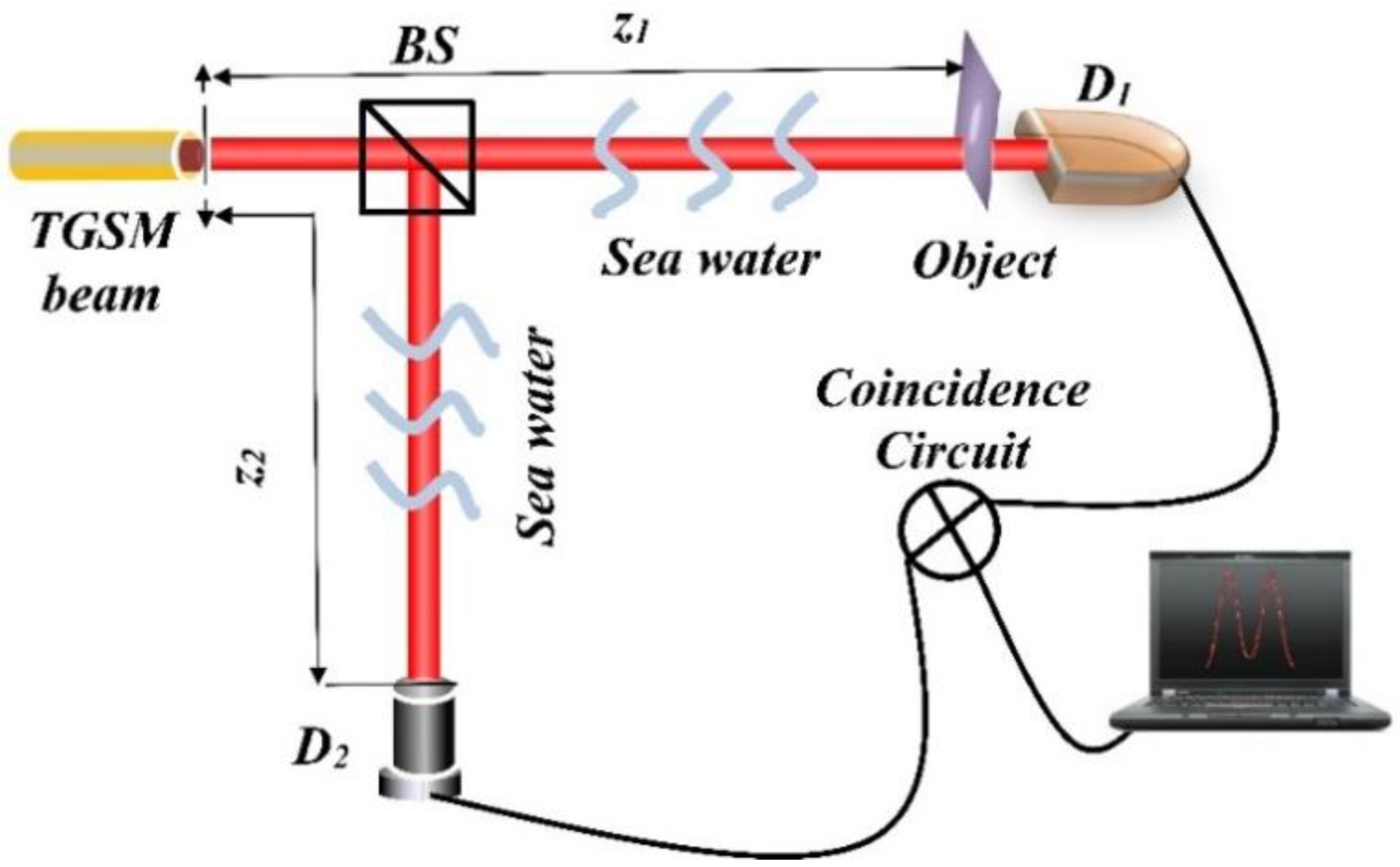
Figure 1 denotes the typical GI setup in an underwater environment. A TGSM beam generated from the source plane first goes towards a 50:50 non-polarized beam splitter (BS), separating into two equal portions. The reflected portion (idle path) propagates through oceanic turbulence and arrives at a detector (
D2). The transmittance portion (signal path) also passes through oceanic turbulence, and arrives at an object. A bucket detector (
D1) is placed against the object to receive all the light intensity scattered from the object. Note that the beam size of the TGSM beam before illuminating the object should be larger than that of the object and the
D1 should put as close as the object to receive all the light from the object if the size of the object is smaller than that of the sensitive area of the detector. Both the distances from the source plane to
D2 and from the source plane to
D1 are
z, i.e.,
z =
z1 =
z2. The output signals from
D1 and
D2 are then sent to a coincidence circuit connected to a personal computer to measure the fourth-order correlation function (i.e., intensity fluctuations).
According to [
35,
40,
42], the cross-spectral density (CSD) function of a TGSM beam in the source plane is given as follows:
Here
, (
i = 1, 2) are two arbitrary position vectors.
Es is the electric field with random fluctuations. The asterisk and angular brackets with subscript “
s” denote the complex conjugate and the ensemble average over source fluctuations.
and
are the beam width and transverse coherence width in the source plane.
k = 2π/λ is the wavenumber of the light beam, and λ is the wavelength.
μ is a real-valued parameter termed as the twist factor, which is a measure of the strength of the twist phase.
denotes the component of the cross product with respect to the propagation z-axis, i.e.,
. The twist factor
μ must satisfy the inequality
due to the non-negative requirement of Equation (1).
Paraxial propagation of the electric field from the source plane to the output plane in linear turbulent media can be explored by the following extended Huygens–Fresnel integral
where
E denotes the random electric field in the output plane, and
h(
r,
u) is the response function between the source plane to the output plane. According to
Figure 1, the functions
h1 in path one and
h2 in path two can be written as
respectively.
H(
u1) in Equation (3) is the transmission function of the object.
in Equations (3) and (4) represents the random complex phase perturbation of spherical wave propagation from (
r, 0) to (
u,
z) induced by the oceanic turbulence.
By applying Equations (1)–(4), the average intensity received by detectors
D1 and
D2 can be expressed as
respectively. The angular brackets with subscript “
M” denote the ensemble average over the fluctuations of turbulence. Under the condition that the oceanic turbulence is isotropic and homogeneous, the second-order statistics of phase perturbations can be represented as [
43]
The parameter
M is expressed as
where
is the one-dimensional power spectrum of refractive index fluctuations given by
Here
κ is the magnitude of three-dimensional spatial frequency vector.
ε is the rate of dissipation of turbulent kinetic energy per unit mass of fluid, usually varying from 10
−2 to 10
−8 m
2/s
3, and
η = 10
−3 m is the Kolmogorov microscale, the function
f takes the form
in Equation (10) is the dissipation rate of mean-square temperature, which may vary from 10
−10 to 10
−4 K
2/s;
ω (−5 <
ω < 0) represents the ratio of temperature and salinity contributions to the refractive index spectrum. In the low bound value, it means that no fluctuations in salinity concentration, while the salinity fluctuations dominate the major role when
ω approaches zero. The other parameters in Equation (10) are set as
,
. The reason for the chosen of these parameter values can be found in [
43] and these values are widely used in the calculation of laser beams propagation in oceanic turbulence.
It is known that one cannot acquire any information of object through measuring the average intensity in path one or two. The reason is that in path one, no object is located, and the bucket detector
D2 only measures the total intensity from the object with no resolution. However, the information of the object can be retrieved by measuring the fourth-order correlation function (FOCF) between
D1 and
D2. According to the optical coherence theory, the FOCF
G(2) between
D1 and
D2 is defined as
In the derivation of Equation (11), it is assumed that the fluctuations induced by the source and the turbulence are statistical independent. On substituting Equations (3) and (4) into Equation (11), it turns out to be
To further simplify Equation (12), it is assumed that the statistics of the source fluctuations obey the Gaussian statistics. Applying the Gaussian moment theorem [
42], the fourth-order statistics can be expressed in terms of summation of second-order statistics, i.e.,
where
, (
i,
j = 1, 2, 3, 4) stands for the second-order statistics of the source, the expression for
is shown in Equation (1). While it is difficult to find the analytical expression for the fourth-order statistics of oceanic turbulence shown in the last term in Equation (12), here we assume that the statistics of turbulence in path one and in path two are independent. The fourth-order statistics of turbulence are reasonably simplified as
On substituting Equations (13) and (14) into Equation (12), we derive the following expression
with
It follows from Equation (15) that the information of the object is contained in
, but it involves eight-folded integrals. Note that the integral functions in Equation (15) or Equation (16) are all exponential functions with quadratic terms. Therefore, it can be greatly simplified with the help of the tensor method [
44]. The terms in the right-hand of Equation (13) have the following alternative tensor forms
where
is one column matrix, the superscript “
T” denotes the transpose of the matrix, and
and
are
matrices, given by
with
Here
,
,
and
are
identity and anti-symmetric matrices, respectively.
The fourth-order statistics induced by the oceanic turbulence can be rewritten as
where
in Equation (22) is an
identity matrix and
. Finally, the tensor form of the product of four response functions in the absence of turbulence is given as
Here
is one column matrix,
On substituting Equations (17), (18), (21), and (23) into Equation (15) we obtain the expression
By applying the following integral formula
which is valid for
n-dimensional vectors
x,
k and a symmetric matrix
A with the positive definite real part, after integrating over
, we have the form
where
and
,
is a
unit matrix. Equations (27) and (28) provide a convenient way for studying the behavior of a ghost image formed with a TGSM beam in the presence of oceanic turbulence.
3. Numerical Results and Discussions
In this section, as numerical examples, we will study the effects of the twist factor and the oceanic turbulence (i.e., the rate of dissipation of mean-square temperature and temperature-salinity balance parameter) on the image visibility and quality in a lensless GI system based on the formulae derived in
Section 2.
For the convenience of analysis, the object in the calculation is the double slits whose transmission function is therefore given by
where
a is the width of each slit and
d is the distance between two slits. Thus, the normalized ghost image function associated with background noise is defined as
The integration over
u1 in Equation (30) means that the detector
D1 is the bucket detector without resolution. On substituting Equations (27)–(29) into Equation (30), we can numerically calculate the image of double slits contained in
g function.
Figure 2a presents the image of double slits in the absence of turbulence (
M = 0) for several different values of the twist factor. The parameters used in the calculation are chosen to be
a = 0.6 mm,
d = 1.2 mm, σ
I0 = 5.0 mm, σ
g0 = 0.4 mm,
λ = 632.8 nm, and
z = 10 m, and kept fixed unless other values are specified. For comparison, we plot in
Figure 2b the corresponding image in the presence of oceanic turbulence. The turbulence parameters are
,
,
One can see that the twist factor has a significant effect on the image visibility and quality, regardless of whether it is in free space or oceanic turbulence. As the value of twist factor increases, the image quality decreases whereas the visibility increases. When the oceanic turbulence is introduced, it has negative effects on the formed image, i.e., the quality and visibility of the image were further degraded compared to those without turbulence.
In general, the visibility and quality of the image are closely related to the transverse coherence width in the planes
u1 and
u2. The smaller the coherence width is, the lower the visibility is and the higher the quality is [
7]. In oceanic turbulence, the evolution of the coherence width of the TGSM beam with propagation distance is closely related to the second-order statistics of the complex phase perturbation induced by turbulence. According to [
45], the relations between the coherence width
at distance z and the turbulence parameters can be expressed by the following analytical formula
with
where
;
is the power spectrum of refractive index fluctuations in oceanic turbulence. Though Equation (31) describes the behavior of the coherence width in atmospheric turbulence in [
45], it also applicable for the case in oceanic turbulence due to that the atmospheric and oceanic turbulence in the analysis all belong to linearly random media. It follows from Equation (31) that when the turbulence is very weak
T << 1 or without turbulence
, it reduces to
. Obviously, the parameter
stands for the increase of coherence width due to the diffraction effect. The first, second, and third term in square brackets in Equation (32) denote the diffractions induced by the twist factor, initial beam width, and initial coherence width during propagation, respectively. The last term is the turbulence-induced extra diffraction effect. However, when the turbulence is strong or the propagation distance is large, the behavior of the coherence width becomes much complicated. The last two terms, which denote the turbulence-induced de-coherence effect, have appreciate values. This effect results in the decrease of the coherence on propagation. Therefore, compared to the case in free space, the coherence width in turbulence increases slowly with propagation distance at first, reaches the maximum value, then starts to decrease with further increases of the propagation distance. One can determine the critical propagation distance where the coherence width reaches the maximum value through the formula:
. This critical value is related by the initial beam parameters and the turbulence parameters. In general, the stronger the turbulence is, the smaller the critical distance is. When the turbulence is strong enough or the propagation distance is sufficiently large, i.e., 1/Δ(
z) << 1, Equation (31) has an asymptotic expression
, implying that the coherence width only depends on the turbulence and decreases with the increase of the propagation distance with
z−1/2.
Figure 2c shows the dependence of coherence width on the twist factor both with and without turbulence at
z = 10 m, and
Figure 2d shows the evolution of the coherence width with propagation distance in turbulence at several twist factors. The parameters in the calculation are the same in
Figure 2a,b. It can be seen that the behavior of the evolution is consistent with our aforementioned analysis.
As shown in
Figure 2c, the coherence width increases with the increase of twist factor both with and without turbulence, while in turbulence, it increases much slower than that without turbulence. That is the reason why the quality of image deteriorates and visibility improves as the twist factor increases (see
Figure 2a or
Figure 2b). However, the visibility and quality in turbulence are worse than that without turbulence under the condition of the same beam parameters when the twist factor is small (
μ < 0.2 m
−1). As the twist factor increases further, i.e.,
μ > 0.3, the quality and visibility of the image in turbulence are almost the same as those without turbulence (compared to the blue dotted curve in
Figure 2a,b). However, the quality of the image seems too low to be applied in practice for
μ > 0.3 m
−1. This phenomenon may be explained by the fact that, in our analysis, the statistics of the turbulence in two paths of GI setup are assumed to be statistically independent, which means that the idle and signal paths suffer the different phase distortions induced by turbulence during propagation at the same time. As a result, the statistical correlations of the two beams at
z =
z1 (just before the object) in the signal path and at
z =
z2 in the idle path are partially destroyed (without turbulence, the statistics of the two beams are exactly the same). Therefore, the quality and visibility all become worse in turbulence compared to those without turbulence. It was shown in [
46] that the partially coherent beams carrying twist phase have the ability to resist the turbulence-induced degradation, reducing the scintillation index (intensity fluctuation), and the larger the twist factor is, the more significant the effect is. That may be the reason the image quality and visibility are almost immune to turbulence in our analysis in the case of large twist factor.
To characterize the image visibility and quality quantitatively, we adopt the parameter
V used in [
31]
where the subscripts “max” and “min” denote the maximum value and minimum value of function
g, respectively. The larger the value of
V is, the higher the visibility of the image is. A new parameter, the correlation coefficient (CC) is introduced to characterized image quality, defined as
where the function
g and
H are defined in Equations (33) and (34), respectively.
E{} is an expectation operator, given by
. It follows from Equation (34) that the denominator can be regarded as the product of the standard deviation of the function
g and
H, and the numerator is the covariance of the function
g and
H. According to the Cauchy–Schwarz inequality, the value of CC is in the range from 0 to 1. When the CC approaches the upper limit, it implies that the ideal ghost image is obtained. As the value of CC decreases, the quality of the image deteriorates gradually.
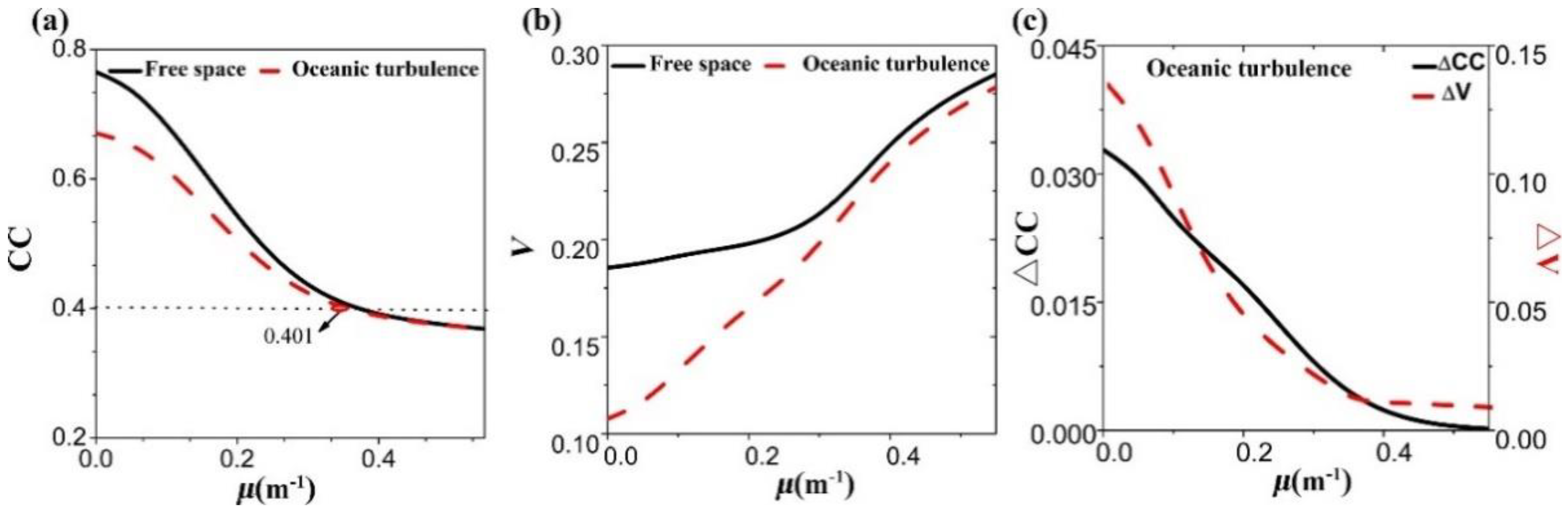
Figure 3a,b illustrate the variation of CC and
V as a function of twist factor, respectively. It can be seen that the value of CC decreases monotonously as the twist factor increases both in free space and in oceanic turbulence. However, the differences of CC between in free space and in oceanic turbulence become smaller with the increase of twist factor, implying that the quality of the image with larger twist factor is less affected by the oceanic turbulence. Especially for the twist factor larger than 0.4 m
−1, the quality of the image seems to be immune to the turbulence, but in this situation, the image of the double slits is completely blurred. Thus, we set a critical value of CC which is 0.401 (see the image plotted with blue dashed dot line in
Figure 2b). Only when the value is larger than 0.401, can the image of double slits be distinguished. As shown in
Figure 3b, the visibility of the image increases as the twist factor increases both in free space and in oceanic turbulence, while in turbulence the visibility is always smaller than that in free space. The reason, as we stated previously, is that the different phase distortions imposed on the beams in two paths results in the visibility degeneration.
In order to show the effects of the oceanic turbulence on the quality and visibility with different twist factors, the parameter named relative difference of quality or visibility is introduced
where the subscripts “
f” and “
t” denote the quality or visibility in free space and in turbulence, respectively. The smaller
or
is, the fewer effects that are induced by the turbulence.
Figure 3c presents the changes in the
and
with the twist factor. It clearly shows that the visibility or quality is less affected by the turbulence as the twist factor increases.
Let us now turn to investigate the influences of the oceanic turbulence such as the dissipation rate of mean-square temperature
, the rate of dissipation of turbulent kinetic energy per unit mass of fluid
ε, and the ratio of temperature and salinity
ω on the characteristics of the image of double slits.
Figure 4 illustrates the image of double slits, the coherence width, the quality and the visibility as a function of
. The other turbulence parameters used in the calculation are
,
. As the value of
increases, the image of double slits blurs gradually. From the change of the coherence width with propagation distance (see in
Figure 4b), the de-coherence effect becomes more and more apparent with the increase of
, indicating that the strength of turbulence increases. As a consequence, the quality of image drops and so does the visibility. The beam with larger twist factor forms the image with higher visibility but with lower quality.
Figure 5 and
Figure 6 show the image of double slits, coherence width, image quality, and visibility against the parameters
ε and
ω, respectively. The turbulence parameters used in
Figure 5 and
Figure 6 are
,
and
,
, respectively. Compared to
, the influences of the
ε and the
ω on the quality or visibility of the image are milder. The formed image is not totally blurred in the varying range of
ε or
ω. Only when the value of
ε is smaller than 10
−7 m
2/s
3 or the
ω is larger than −2, the quality of the image starts to drop. This varying is consistent with the changes of the coherence width shown in
Figure 5b and
Figure 6b. The beam with a large twist factor always keeps the large coherence width at the detected plane, which leads to the quality of the image being lower than that of the small twist factor, while in the case of visibility this is reversed. Therefore, one can use the twist phase to improve the visibility of the image, under the situation that the quality of the image is acceptable.
At last, we investigate the effects of the propagation distance on the quality and visibility of the image of the double slits.
Figure 7 shows the variation of the image of the double slits and the quality and visibility with propagation distance both in free space and in turbulence. In the calculation, the turbulent parameters are chosen to be
,
,
. For the case of free space, the quality/visibility of image decreases/increases as the propagation distance increases, as expected. The reason is that the coherence width of the beam increases as the propagation distance increases due to the diffraction effect. Under the same propagation distance, the coherence width with a large twist factor is larger than that with a small twist factor (see in
Figure 7d). Thus, the beam with a large twist factor has high visibility and low quality. In the presence of oceanic turbulence, the change rules of the image quality and visibility are similar to those in free space. However, the image quality for
μ = 0 in turbulence drops much faster than that in free space. As the twist factor increases, the variations of the image quality with propagation distance in turbulence are gradually close to their variations in free space, which means that the image with large twist factor is less affected by the turbulence. In spite of this, the large twist factor will degrade the beam quality and even totally blur the image; one may choose a tradeoff twist factor for practical use where the image quality and visibility are acceptable.
Finally, we should emphasize that the results including the image of double slits, image quality, and visibility obtained in this article correspond to those from the numerical simulation with random mode decomposition when the number of random modes (measurements)
N is sufficiently large or infinity. In fact, there are two methods to calculate the results for the ghost image in numerical calculation/simulation. One directly uses the CSD function of the partially coherent beam (random beam) [
24,
31,
32], and another is based on random mode decomposition of the beam [
30,
47,
48]. The CSD function shown in Equation (1) can be considered as the results for the ensemble average over the random fluctuations. In the latter method, the random beam is usually expressed as
where
En represents the one realization of the random field. Under this scenario, the partially coherent beam is regarded as the
N realizations of the incoherent superposition of the random fields, and the derived quantities depend on the number of realizations (measurements). Only when the number of realization is sufficiently large (approaches to infinity in theory), Equations (1) and (37) may establish the relation
Therefore, all the results derived in our article are the cases of the number of measurement N being large enough (approaching infinity).


