Bayesian Estimation of Residual Life for Weibull-Distributed Components of On-Orbit Satellites Based on Multi-Source Information Fusion

Abstract

Residual life estimation is an important problem in reliability engineering. Traditional methods, which are based on time-to-failure distribution, have limitations for components of on-orbit satellites characterized as high reliability with small sample size. Various types of reliability information can be collected during test and operation, including historical lifetime data, degradation data, similar data, expert information, etc. Therefore, making full use of multi-source information is meaningful for improving estimation precision. However, research on residual life estimation by fusing multi-source information is rare. No study has examined the overall process of fusing all of the different kinds of information. In this paper, a Bayesian method is presented to estimate the residual life of Weibull-distributed components of on-orbit satellites by fusing all the collected information. Prior distributions are determined using different kinds of information. After fusing the field data, posterior distributions can be obtained corresponding to each prior distribution. Then, the joint posterior distribution is the weighted sum of these posterior distributions with weights calculated using the second Maximum Likelihood Estimation (ML-II) method. Consistency is tested to guarantee the safety of the information fusion. Furthermore, residual life is estimated by the proposed sample-based method including both the Bayesian estimate and credible interval (CI). A Monte Carlo simulation study is conducted to demonstrate the proposed methods and shows that the Bayesian method is satisfactory and robust. Finally, a published dataset of the momentum wheel in a satellite is analyzed to illustrate the application of the method.

1. Introduction

Residual life estimation is crucial in reliability engineering [1,2] and is the key technology for prognostic and health management (PHM), used to analyze, guarantee, and improve safety and reliability [3]. Given the cumulative distribution function (CDF) F(t), probability density function (PDF) f(t) of a component and the lifetime T, the CDF of the residual life F_τ (t) at time τ, can be calculated by

$$F_{\tau }\left(t\right)=P\left(T<t+\tau |T>\tau \right)=\frac{P\left(\tau <T<t+\tau \right)}{P\left(T>\tau \right)}=\frac{F\left(t+\tau \right)-F\left(\tau \right)}{1-F\left(\tau \right)} .$$

(1)

Hence, the PDF of the residual life at time τ is given by

$$f_{\tau }\left(t\right)=\frac{d{F}_{\tau }\left(t\right)}{dt}=\frac{f\left(t+\tau \right)}{1-F\left(\tau \right)} .$$

(2)

Then, the point estimation of the residual life can be represented as

$${\mu }_{\tau }={\displaystyle \underset{0}{\overset{\infty }{\int }}t{f}_{\tau }(t)dt}.$$

(3)

Weibull distributions are widely used [4,5]. Therefore, in this study, we assume the lifetime of the on-orbit component follows the Weibull distribution, denoted by W($\lambda ,\beta$), with the CDF [6]

$$F(t;\lambda ,\beta )=1-e^{-\lambda t^{\beta }},\hspace{1em}\hspace{1em}t\ge 0,\lambda >0,\beta >0.$$

(4)

The residual life PDF can be obtained by substituting Equation (4) into Equation (2), which can be written as [5]

$$f_{\tau }\left(t;\lambda ,\beta \right)=\frac{f\left(t+\tau \right)}{1-F\left(\tau \right)}=\lambda \beta {\left(t+\tau \right)}^{\beta -1}\exp \left(\lambda {\tau }^{\beta }-\lambda {\left(t+\tau \right)}^{\beta }\right).$$

(5)

With the development of the techniques of science and technology, the components in satellites are highly reliable. Therefore, applications of traditional methods based on failure times are limited [7]. However, multi-source information can be collected for these components [8], including historical lifetime data, degradation data, similar data, and expert information. The Bayesian method could be a useful tool for the information fusion. Because of its strong ability at data fusion [9], it has received considerable attention in various engineering fields [10,11].

For highly reliable components, it is difficult to estimate the residual life with data containing a small number of failures and even zero failure. However, the available degradation data could reflect the real-time state of components and could be used to enrich the information for residual life estimation [12]. For example, a hierarchical Bayesian model was built and effectively fitted the nonlinear paths of organic light-emitting diodes [13]. Parameters of the Wiener process and the field data were fused to obtain the posterior distributions of degradation parameters [14]. In addition, a systematic method for using a degradation-based model selection to analyze Bayesian reliability was discussed by Li et al. [15]. Additionally, Bernoulli data, lifetime data, and degradation data were integrated to improve the accuracy of reliability prediction [16]. Parameters of the degradation model were determined by fusing prior degradation information and prior lifetime data, and prior distribution was updated by the field degradation data [17]. By synthesizing multi-source data, including bivariate degradation data and lifetime data, remaining useful life (RUL) was estimated for a satellite rechargeable lithium battery [2]. The inverse Gaussian process was used to analyze the accelerated degradation model and both the Jeffreys prior and reference prior were derived and compared [18]. Based on the functional principal component analysis (PCA) and the Bayesian method, a new prediction method for Li ion battery residual lifetime evaluation was presented [19].

Simultaneously, historical lifetime data and similar data can also obviously provide more reliability information. Historical lifetime data, often obtained before test and use, and the similar data are usually used to determine prior distribution based on empirical Bayes (EB) [20] and linear empirical Bayes (LEB) methods [21]. In practical engineering, conjugate prior is also commonly used [22]. The moment method, as well as the ML-II method, are typically used to determine the parameters of prior distribution [23]. Degradation data and historical lifetime data were fused to estimate the residual life [24]. Based on the previous number of failures, the failure rate was obtained from a new software reliability model [25]. The reliability of Weibull-distributed components was evaluated under the small sample sizes and zero-failure data by fusing both the target and similar products [26]. By fusing the prior information of similar products, the modified Bayesian method of assessing the reliability of binomial components was proposed [27].

Expert information is also valuable especially when the field data are insufficient [28]. Integration of expert knowledge into lifetime estimation was presented [29]. An expert-judgement process for fusing multi-source prior information was developed by Yang et al. [30]. Various available sources of expert knowledge and data, at both subsystem and system levels, were integrated [31], and methods for fusing lifetime data and expert information were discussed [32].

Prior information is important in Bayesian theory. After obtaining prior distributions according to different kinds of reliability information, the next step is to aggregate these prior distributions to eliminate the uncertainty of each multi-source information. Existing methods concerning the prior distribution fusion are based on confidence level [33], correlation function [34], sufficiency measure [35], expert judgement [36], maximum entropy-moment estimation [37], fuzzy logic operators [38], maximum likelihood principle [39], and the ML-II method [40]. Peng [41,42] has made special contributions to this field.

These models and methodologies have formed a solid foundation for the Bayesian estimation of residual life. However, after extensive literature review, we found that (i) although work has been done on Bayesian theory and its applications, most of the existing literature concentrates mainly on certain aspects. The overall process and detailed illustration of the Bayesian method by fusing all this multi-source information simultaneously have rarely been presented or analyzed. (ii) Research on residual life estimation by fusing multi-source information is rare and needs further study. To fill the gap of the existing research, a multi-source information fusion approach based on the Bayesian theory is proposed to estimate the residual life of Weibull-distributed components of on-orbit satellites by fusing historical lifetime data, degradation data, similar data, and expert information. Both the Bayesian estimate and CI are considered.

The rest of this paper is organized as follows. Multi-source information and the Bayesian model are introduced in Section 2. Section 3 contains the determination of prior distributions of multi-source information. In Section 4, we describe how posterior distributions are obtained and fused after a consistency test, and the residual life is estimated. Section 5 describes the Monte Carlo simulation study, followed by the validation using an illustrative example in Section 6. Finally, the paper is concluded in Section 7.

2. Multi-Source Information and the Bayesian Model

In this section, various kinds of reliability information and the Bayesian method are introduced. The following reliability information can be collected for components of on-orbit satellites according to engineering experience.

(i).

Field data $D=\{t_1^D,t_2^D,\cdots ,t_r^D,t_{r+1}^D,\cdots ,t_n^D\}$ are collected during the operation of target components, where n represents the sample size, $\{t_1^D,t_2^D,\cdots ,t_r^D\}$ are the failure times of the field data, and $\{t_{r+1}^D,\cdots ,t_n^D\}$ are the censored data. It should be noted that the censored data in this paper means the correct censored data.

(ii).

Historical lifetime data $D_H=\{t_1^H,t_2^H,\cdots ,t_d^H,t_{d+1}^H,\cdots ,t_p^H\}$ are data for the end of operation of the same kinds of existing products, where p represents the sample size, $\{t_1^H,t_2^H,\cdots ,t_d^H\}$ are the failed data, and $\{t_{d+1}^H,\cdots ,t_p^H\}$ are the censored data.

(iii).

Similar data $D_S=\{t_1^S,t_2^S,\cdots ,t_k^S,t_{k+1}^S,\cdots ,t_m^S\}$ are the data of similar components, where m denotes the sample size, $\{t_1^S,t_2^S,\cdots ,t_k^S\}$ are the failed data, $\{t_{k+1}^S,\cdots ,t_m^S\}$ are the censored data, and ρ is the inheritance factor that reflects the similarity with the target components.

(iv).

Degradation data $X=\{X_1,X_2,\cdots ,X_l\}$ are collected from l components during the operation for a single parameter, where $X_d=\{X_{d1},X_{d2},\cdots ,X_{dh}\}$ ($d=1,2,\dots l$) are observed at time $d1,d2,\cdots ,dh$.

(v).

Expert information is provided by expert experience, and usually includes two forms: (a) Point estimation $R_0$ of reliability at time ${\tau }_0$ and (b) the lower confidence limit $R_L$ for the reliability at time ${\tau }_0$ with confidence level $100(1-\gamma )\%$.

There are four major steps to the Bayesian method proposed in this paper: (i) Prior distributions are determined by historical lifetime data, degradation data, similar data, and expert information, which are denoted by ${\pi }_i(\lambda ,\beta )$ ($i=1,2,3,4$); (ii) Corresponding posterior distributions ${\pi }_i(\lambda ,\beta |D)$ ($i=1,2,3,4$) are obtained by fusing the field data; (iii) Fusion weights are calculated using the ML-II method, and the joint posterior distribution $\pi (\lambda ,\beta |D)$ can be obtained; and (iv) Residual life can be estimated.

3. Prior Distributions of Multi-Source Information

In this section, the methods used for obtaining prior distributions based on multi-source information are outlined.

3.1. Prior Distribution Obtained by Expert Information

Reliability at time τ is

$$R_{\tau }=\exp \left(-\lambda {\tau }^{\beta }\right).$$

(6)

In this paper, using the idea of the conjugate prior, the negative log gamma (NLG) distribution is assumed to be the prior distribution of $R_{\tau }$ with the PDF [43]

$$\pi (R_{\tau })=\frac{b^a}{\Gamma (a)}{\left(R_{\tau }\right)}^{b-1}{\left(-\ln R_{\tau }\right)}^{a-1}.$$

(7)

To estimate the residual life, the NLG distribution for $R_{\tau }$ should firstly be transformed to the prior distribution of the Weibull parameters $\lambda$ and $\beta$. The derivative of Equation (6) with respect to $\lambda$ is

$$\frac{d{R}_{\tau }}{d\lambda }=-{\tau }^{\beta }\exp \left\{-\lambda {\tau }^{\beta }\right\}<0.$$

(8)

According to Equation (8), $R_{\tau }$ decreases with $\lambda$. Hence, we have

$$P(\lambda <x)=P\left(R_{\tau }>\exp \left(-x{\tau }^{\beta }\right)\right)={\displaystyle {\int }_{\exp \left(-x{\tau }^{\beta }\right)}^1\pi (R_{\tau })d{R}_{\tau }}.$$

(9)

By taking the derivative of Equation (9) with respect to $x$, we have

$$f_{\lambda }(x)=\frac{{\left(b{\tau }^{\beta }\right)}^a}{\Gamma (a)}{x}^{a-1}\exp \left(-b{\tau }^{\beta }x\right).$$

(10)

Then,

$$\pi (\lambda |\beta )=\frac{{\left(b{\tau }^{\beta }\right)}^a}{\Gamma (a)}{x}^{a-1}\exp \left(-b{\tau }^{\beta }x\right).$$

(11)

It is assumed that [43]

$$\pi (\beta )=\frac{1}{{\beta }_2-{\beta }_1},\beta \in [{\beta }_1,{\beta }_2],$$

(12)

then we obtain the prior distribution of $\lambda$ and $\beta$ as

$$\pi (\lambda ,\beta )=\frac{1}{{\beta }_2-{\beta }_1}\frac{{\left(b{\tau }^{\beta }\right)}^a}{\Gamma (a)}{\lambda }^{a-1}\exp \left(-b{\tau }^{\beta }\lambda \right).$$

(13)

where $\lambda \in [0,\infty ]$ and $\beta \in [{\beta }_1,{\beta }_2]$. The next step is to determine the values of $a$ and $b$ by expert information.

For case (a) of expert information described in the reliability information (v) of Section 2, we have

$${\displaystyle {\int }_0^1{R}_{{\tau }_0}\pi (R_{{\tau }_0})d{R}_{{\tau }_0}}=R_0.$$

(14)

By using the maximum entropy method (MEM), this problem could be represented by

$$\{\begin{array}{l}\max H=-{\displaystyle {\int }_0^1\pi (R_{{\tau }_0})\ln \left[\pi (R_{{\tau }_0})\right]d{R}_{\tau }}\\ s.t.{\displaystyle {\int }_0^1{R}_{{\tau }_0}\pi (R_{{\tau }_0})d{R}_{{\tau }_0}}=R_0\end{array}.$$

(15)

This constrained optimization problem can be simplified as

$$\{\begin{array}{l}\max H=-a_1\ln \left(b_1\right)+\ln \left(\Gamma (a_1)\right)+\frac{a_1(b_1-1)}{b_1}-\frac{(a_1-1){b_1}^{a_1}}{\Gamma (a_1)}B\\ s.t.{\left(\frac{b_1}{b_1+1}\right)}^{a_1}=R_0\end{array},$$

(16)

where $B={\displaystyle {\int }_0^1{\left(R_{{\tau }_0}\right)}^{b_1-1}{\left(-\ln R_{{\tau }_0}\right)}^{a_1-1}\cdot \ln \left[-\ln \left(R_{{\tau }_0}\right)\right]d{R}_{{\tau }_0}}$. $a_1$ and $b_1$ satisfy $a_1=\frac{\ln \left(R_0\right)}{\ln \left(b_1\right)-\ln \left(b_1+1\right)}$. Then Equation (16) could be turned into a one-dimension optimization.

In addition, for case (b) of expert information, if the $100(1-\gamma )\%$ lower confidence limit $R_L$ for the reliability at time ${\tau }_0$ is given, then

$${\displaystyle {\int }_{R_L}^1\pi (R_{{\tau }_0})d{R}_{{\tau }_0}}=1-\gamma .$$

(17)

Similarly, the constrained optimization problem can be represented as

$$\{\begin{array}{l}\max H=-{\displaystyle {\int }_0^1\pi (R_{{\tau }_0})\ln \left[\pi (R_{{\tau }_0})\right]d{R}_{{\tau }_0}}\\ s.t.{\displaystyle {\int }_{R_L}^1\pi (R_{{\tau }_0})d{R}_{{\tau }_0}}=\gamma \end{array},$$

(18)

which can be simplified as

$$\{\begin{array}{l}\max H=-a_1\ln \left(b_1\right)+\ln \left(\Gamma (a_1)\right)+\frac{a_1(b_1-1)}{b_1}-\frac{(a_1-1){b_1}^{a_1}}{\Gamma (a_1)}B\\ s.t.I_{-b_1\ln (R_L)}(a_1)=1-\gamma \end{array},$$

(19)

where

$$I_{-b_1\ln (R_L)}(a_1)=\frac{1}{\Gamma (a_1)}{\displaystyle {\int }_0^{-b_1\ln (R_L)}{e}^{-t}{t}^{a_1-1}dt}$$

(20)

is the incomplete gamma function. Parameters $a_1$ and $b_1$ can be calculated by intelligent optimization algorithms.

According to Equation (13), the prior distribution using expert information can be represented by

$${\pi }_1(\lambda ,\beta )=\frac{1}{{\beta }_2-{\beta }_1}\frac{{\left(b_1{\tau }^{\beta }\right)}^{a_1}}{\Gamma (a_1)}{\lambda }^{a_1-1}\exp \left(-b_1{\tau }^{\beta }\lambda \right),\lambda \in [0,\infty ],\beta \in [{\beta }_1,{\beta }_2].$$

(21)

3.2. Prior Distribution Obtained by Historical Lifetime Data

According to the definition of the non-informative prior, we have

$$\pi \left(R_{\tau }\right)=\{\begin{array}{l}\mathrm{NLG}\left(0,0\right),d\ne 0\\ \mathrm{NLG}(1/2,0),d=0\end{array}$$

(22)

by setting $a=\{\begin{array}{l}0,d\ne 0\\ 1/2,d=0\end{array}$ and $b=0$ in Equation (7) [43]. Because likelihood function of the historical lifetime data can be given by

$$L\left(D_H|\lambda ,\beta \right)={\lambda }^d{\beta }^d{(E^H)}^{\beta -1}\exp \left(-\lambda F^{H(\beta )}\right),$$

(23)

where $E^H={\displaystyle \prod _{i=1}^d{t}_i^H}$ and $F^{H(\beta )}={\displaystyle \sum _{i=1}^p{(t_i^H)}^{\beta }}$, we can use the Bayesian theory to integrate the prior distribution ${\pi }_2(\lambda ,\beta )$, which takes the form of Equation (13), and the likelihood function as

$$\begin{array}{cc}& {\pi }_2(\lambda ,\beta |D_H)\hfill \\ \hfill =& \frac{{\pi }_2(\lambda ,\beta )\cdot L\left(D_H|\lambda ,\beta \right)}{{\displaystyle {\int }_{{\beta }_1}^{{\beta }_2}{\displaystyle {\int }_0^{\infty }{\pi }_2(\lambda ,\beta )\cdot L\left(D_H|\lambda ,\beta \right)d\lambda d\beta }}}\hfill \\ \hfill =& \frac{{\tau }^{a_2\beta }{\beta }^d{(E^H)}^{\beta -1}{\lambda }^{d+a_2-1}\exp \left[-\lambda (F^H{}^{(\beta )}+b_2{\tau }^{\beta })\right]}{{\displaystyle {\int }_{{\beta }_1}^{{\beta }_2}{\displaystyle {\int }_0^{\infty }{\tau }^{a_2\beta }{\beta }^d{(E^H)}^{\beta -1}{\lambda }^{d+a_2-1}\exp \left[-\lambda (F^H{}^{(\beta )}+b_2{\tau }^{\beta })\right]}d\lambda d\beta }}\hfill \\ \hfill =& \frac{{\tau }^{a_2\beta }{\beta }^d{(E^H)}^{\beta -1}{\lambda }^{d+a_2-1}\exp \left[-\lambda (F^H{}^{(\beta )}+b_2{\tau }^{\beta })\right]}{{\displaystyle {\int }_{{\beta }_1}^{{\beta }_2}{\tau }^{a_2\beta }{\beta }^d{(E^H)}^{\beta -1}\frac{\Gamma (d+a_2)}{{(F^H{}^{(\beta )}+b_2{\tau }^{\beta })}^{d+a_2}}d\beta }},\hfill \end{array}$$

(24)

where $E^H={\displaystyle \prod _{i=1}^d{t}_i^H}$, $F^H{}^{(\beta )}={\displaystyle \sum _{i=1}^p{(t_i^H)}^{\beta }}$, $a_2=\{\begin{array}{l}0,d\ne 0\\ 1/2,d=0\end{array}$, and $b_2=0$. This is the determined prior distribution for the historical lifetime data.

3.3. Prior Distribution Obtained by Degradation Data

Assuming that the degradation process X(t) has an increasing tendency, and given the degradation threshold $D$, the failure time can be defined as

$$T=\inf \{t|X(t)\ge D\}.$$

(25)

The failure distribution is

$$P\left(T\le t\right)=P\left(\underset{0\le s\le t}{\sup }X\left(s\right)\ge D\right),$$

(26)

where $\underset{0\le s\le t}{\sup }X\left(s\right)$ represents the maximum value of degradation data, and $X(s)$ in the time interval of $[0,t]$.

The next step is to model the degradation data $X=\{X_1,X_2,\cdots ,X_l\}$. In the existing literature, the degradation path model, degradation distribution model, and stochastic process models are widely used [22]. The failure times of l components $D_G=\{t_1^G,t_2^G,\cdots t_l^G\}$ can be predicted by Equation (25). Then, the prior distribution ${\pi }_3(\lambda ,\beta )$ can be similarly determined using the method described in Section 3.2.

3.4. Prior Distribution Obtained by Similar Data

Assuming the prior distribution of the similar data takes the form

$${\pi }_4(\lambda ,\beta )=\rho {\pi }_{41}(\lambda ,\beta )+\left(1-\rho \right){\pi }_{42}(\lambda ,\beta ),$$

(27)

where ${\pi }_{41}(\lambda ,\beta )$ is the prior distribution of inheritance and ${\pi }_{42}(\lambda ,\beta )$ is the updated prior distribution. The former depicts the similarity and could be determined using the same method proposed in Section 3.2 as

$${\pi }_{41}(\lambda ,\beta )=\frac{{\tau }^{a_{41}\beta }{\beta }^k{U}^{\beta -1}{\lambda }^{k+a_{41}-1}\exp \left[-\lambda (V^{(\beta )}+b_{41}{\tau }^{\beta })\right]}{{\displaystyle {\int }_{{\beta }_1}^{{\beta }_2}{\tau }^{a_{41}\beta }{\beta }^k{U}^{\beta -1}\frac{\Gamma (k+a_{41})}{{(V^{(\beta )}+b_{41}{\tau }^{\beta })}^{k+a_{41}}}d\beta }},$$

(28)

where $U={\displaystyle \prod _{i=1}^k{t}_i^S}$, $V^{(\beta )}={{\displaystyle \sum _{i=1}^m(t_i^S)}}^{\beta }$, $a_{41}=\{\begin{array}{l}0,k\ne 0\\ 1/2,k=0\end{array}$, and $b_{41}=0$. In addition, ${\pi }_{42}(\lambda ,\beta )$ could describe the uncertainty and difference in the form of

$${\pi }_{42}(\lambda ,\beta )=\frac{1}{{\beta }_2-{\beta }_1}\frac{{\left(b_{42}{\tau }^{\beta }\right)}^{a_{42}}}{\Gamma (a_{42})}{\lambda }^{a_{42}-1}\exp \left(-b_{42}{\tau }^{\beta }\lambda \right),\lambda \in [0,\infty ],\beta \in [{\beta }_1,{\beta }_2].$$

(29)

Generally, ${\pi }_{42}(\lambda ,\beta )$ is assumed to follow a non-informative prior distribution with $a_{42}=1$, and $b_{42}=1$. Then, we have

$${\pi }_{42}(\lambda ,\beta )=\frac{1}{{\beta }_2-{\beta }_1}{\tau }^{\beta }\exp \left(-{\tau }^{\beta }\lambda \right).$$

(30)

4. Information Fusion and Residual Life Estimation

In this section, different posterior distributions corresponding to each prior distribution are firstly obtained by fusing field data. Then the Bayesian credible interval method is used to complete a consistency test, which is essential for guaranteeing that all the fused data are from the same population. Furthermore, the residual life is estimated after integrating all the information.

4.1. Joint Prior Distribution and Joint Posterior Distribution

As different prior distributions of historical lifetime data, degradation data, similar data and expert information are obtained, the fusion of prior distributions is necessary to decrease uncertainty. Usually, the joint prior distribution $\pi (\lambda ,\beta )$ can be calculated by

$$\pi (\lambda ,\beta )={\displaystyle \sum _{i=1}^4{\epsilon }_i{\pi }_i(\lambda ,\beta )},$$

(31)

where ${\epsilon }_i$ is the fusion weight of the ith prior distribution and ${\displaystyle \sum _{i=1}^4{\epsilon }_i}=1$. The core problem for fusing these different prior distributions is to determine the weight ${\epsilon }_i$. Considering that the ML-II method is simple, it is adopted in this paper to determine the weight ${\epsilon }_i$ and to fuse prior distributions. Under the prior distribution ${\pi }_i(i=1,2,3,4)$, the marginal likelihood function of field data $D=\{t_1^D,t_2^D,\cdots ,t_r^D,t_{r+1}^D,\cdots ,t_n^D\}$ is

$$L(D|{\pi }_i)={\displaystyle \prod _{j=1}^{r}f(t_j^D|{\pi }_i)}{\displaystyle \prod _{j=r+1}^{n}R(t_j^D|{\pi }_i)},$$

(32)

where

$$f(t_j^D|{\pi }_i)={\displaystyle {\int }_{{\beta }_1}^{{\beta }_2}{\displaystyle {\int }_0^{\infty }f(t_j^D|\lambda ,\beta ){\pi }_i(\lambda ,\beta )d\lambda d\beta }},$$

(33)

and

$$R(t_j^D|{\pi }_i)={\displaystyle {\int }_{{\beta }_1}^{{\beta }_2}{\displaystyle {\int }_0^{\infty }R(t_j^D|\lambda ,\beta ){\pi }_i(\lambda ,\beta )d\lambda d\beta }}.$$

(34)

The bigger the $L(D|{\pi }_i)$, the bigger the fusion weight of ${\pi }_i$. Then, we have

$${\epsilon }_i=\frac{L(D|{\pi }_i)}{{\displaystyle \sum _{k=1}^{4}L(D|{\pi }_k)}},i=1,2,3,4.$$

(35)

Then, the joint prior distribution can be obtained using Equation (31). Let $P(D|\lambda ,\beta )$ represent the likelihood function of field data, by using Equations (31) and (35), we obtain

$$\begin{array}{cc}\hfill \pi (\lambda ,\beta |D)& ={\displaystyle \sum _{i=1}^4\left\{\frac{\frac{L(D|{\pi }_i)}{{\displaystyle \sum _{i=1}^{4}L(D|{\pi }_i)}}{\displaystyle {\int }_{{\beta }_1}^{{\beta }_2}{\displaystyle {\int }_0^{\infty }{\pi }_i(\lambda ,\beta )P(D|\lambda ,\beta )d\lambda d\beta }}}{{\displaystyle \sum _{i=1}^4\frac{L(D|{\pi }_i)}{{\displaystyle \sum _{i=1}^{4}L(D|{\pi }_i)}}{\displaystyle {\int }_{{\beta }_1}^{{\beta }_2}{\displaystyle {\int }_0^{\infty }{\pi }_i(\lambda ,\beta )P(D|\lambda ,\beta )d\lambda d\beta }}}}{\pi }_i(\lambda ,\beta |D)\right\}}\hfill \\ & ={\displaystyle \sum _{i=1}^4\left\{\frac{L(D|{\pi }_i){\displaystyle {\int }_{{\beta }_1}^{{\beta }_2}{\displaystyle {\int }_0^{\infty }{\pi }_i(\lambda ,\beta )P(D|\lambda ,\beta )d\lambda d\beta }}}{{\displaystyle \sum _{i=1}^4\left[L(D|{\pi }_i){\displaystyle {\int }_{{\beta }_1}^{{\beta }_2}{\displaystyle {\int }_0^{\infty }{\pi }_i(\lambda ,\beta )P(D|\lambda ,\beta )d\lambda d\beta }}\right]}}{\pi }_i(\lambda ,\beta |D)\right\}}.\hfill \end{array}$$

(36)

When $w_i=\frac{L(D|{\pi }_i){\displaystyle {\int }_{{\beta }_1}^{{\beta }_2}{\displaystyle {\int }_0^{\infty }{\pi }_i(\lambda ,\beta )P(D|\lambda ,\beta )d\lambda d\beta }}}{{\displaystyle \sum _{i=1}^4\left[L(D|{\pi }_i){\displaystyle {\int }_{{\beta }_1}^{{\beta }_2}{\displaystyle {\int }_0^{\infty }{\pi }_i(\lambda ,\beta )P(D|\lambda ,\beta )d\lambda d\beta }}\right]}}$, we have

$$\pi (\lambda ,\beta |D)={\displaystyle \sum _{i=1}^4{w}_i{\pi }_i(\lambda ,\beta |D)},$$

(37)

where ${\pi }_i(\lambda ,\beta |D)$ and ${\displaystyle {\int }_{{\beta }_1}^{{\beta }_2}{\displaystyle {\int }_0^{\infty }{\pi }_i(\lambda ,\beta )P(D|\lambda ,\beta )d\lambda d\beta }}$ are the posterior distribution and the marginal PDF of the ith prior distribution.

Equation (37) indicates that the joint posterior distribution is equal to the weighted sum of posterior distributions obtained from the corresponding prior distributions. Therefore, it is much easier to obtain the joint posterior distribution, as it can be transformed to determine each posterior distribution for each prior distribution.

4.2. Posterior Distributions of Multi-Source Information

In this subsection, the posterior distributions of historical lifetime data, degradation data, similar data and expert information are described, respectively.

4.2.1. Posterior Distribution of Expert Information

Similar to Equation (23), the likelihood function of field data is

$$P(D|\lambda ,\beta )={\lambda }^r{\beta }^r{M}^{\beta -1}\exp \left(-\lambda N^{(\beta )}\right),$$

(38)

where $M={\displaystyle \prod _{i=1}^r{t}_j^D}$ and $N^{(\beta )}={\displaystyle \sum _{i=1}^n{(t_j^D)}^{\beta }}$. Then, the posterior distribution of expert information is

$$\begin{array}{cc}& {\pi }_1(\lambda ,\beta |D)\hfill \\ \hfill =& \frac{\frac{1}{{\beta }_2-{\beta }_1}\frac{{\left(b_1{\tau }^{\beta }\right)}^{a_1}}{\Gamma (a_4)}{\lambda }^{a_1-1}\exp \left(-b_1{\tau }^{\beta }\lambda \right)\cdot {\lambda }^r{\beta }^r{M}^{\beta -1}\exp \left(-\lambda N^{(\beta )}\right)}{{\displaystyle {\int }_{{\beta }_1}^{{\beta }_2}\left({\displaystyle {\int }_0^{\infty }\frac{1}{{\beta }_2-{\beta }_1}\frac{{\left(b_1{\tau }^{\beta }\right)}^{a_1}}{\Gamma (a_1)}{\lambda }^{a_1-1}\exp \left(-b_1{\tau }^{\beta }\lambda \right)\cdot {\lambda }^r{\beta }^r{M}^{\beta -1}\exp \left(-\lambda N^{(\beta )}\right)d\lambda }\right)d\beta }}\hfill \\ \hfill =& \frac{{\left(b_1{\tau }^{\beta }\right)}^{a_1}{\beta }^r{M}^{\beta -1}{\lambda }^{a_1+r-1}\exp \left(-\lambda \left(b_1{\tau }^{\beta }+N^{(\beta )}\right)\right)}{{\displaystyle {\int }_{{\beta }_1}^{{\beta }_2}\left({\displaystyle {\int }_0^{\infty }{\left(b_1{\tau }^{\beta }\right)}^{a_1}{\beta }^r{M}^{\beta -1}{\lambda }^{a_1+r-1}\exp \left(-\lambda \left(b_1{\tau }^{\beta }+N^{(\beta )}\right)\right)d\lambda }\right)d\beta }}\hfill \\ \hfill =& \frac{{\left(b_1{\tau }^{\beta }\right)}^{a_1}{\beta }^r{M}^{\beta -1}{\lambda }^{a_1+r-1}\exp \left(-\lambda \left(b_1{\tau }^{\beta }+N^{(\beta )}\right)\right)}{{\displaystyle {\int }_{{\beta }_1}^{{\beta }_2}{\left(b_1{\tau }^{\beta }\right)}^{a_1}{\beta }^r{M}^{\beta -1}\frac{\Gamma (a_1+r)}{{\left(b_1{\tau }^{\beta }+N^{(\beta )}\right)}^{a_1+r}}d\beta }}.\hfill \end{array}$$

(39)

To determine the fusion weight in Equation (37), the marginal likelihood function and marginal PDF of field data under ${\pi }_1(\lambda ,\beta )$ should be calculated. For the failure time of field data ($t_j^D$, $j\le r$ ), the failure probability at time $t_j^D$ is

$$\begin{array}{cc}& f(t_j^D|{\pi }_1(\lambda ,\beta ))\hfill \\ \hfill =& \frac{1}{{\beta }_2-{\beta }_1}{\displaystyle {\int }_{{\beta }_1}^{{\beta }_2}{\displaystyle {\int }_0^{\infty }\lambda \beta {(t_j^D)}^{\beta -1}\exp [-\lambda {(t_j^D)}^{\beta }]\cdot \frac{{\left(b_1{\tau }^{\beta }\right)}^{a_1}}{\Gamma (a_1)}{\lambda }^{a_1-1}\exp \left(-b_1{\tau }^{\beta }\lambda \right)d\lambda }d\beta }\hfill \\ \hfill =& \frac{1}{{\beta }_2-{\beta }_1}{\displaystyle {\int }_{{\beta }_1}^{{\beta }_2}\beta {(t_j^D)}^{\beta -1}\cdot \frac{{\left(b_1{\tau }^{\beta }\right)}^{a_1}}{\Gamma (a_1)}\frac{\Gamma (a_1+1)}{{\left(b_1{\tau }^{\beta }+t_j^{\beta }\right)}^{a_1+1}}d\beta }\hfill \\ \hfill =& \frac{1}{{\beta }_2-{\beta }_1}{\displaystyle {\int }_{{\beta }_1}^{{\beta }_2}{a}_1{(t_j^D)}^{\beta -1}\beta \frac{{\left(b_1{\tau }^{\beta }\right)}^{a_1}}{{\left(b_1{\tau }^{\beta }+{(t_j^D)}^{\beta }\right)}^{a_1+1}}d\beta }.\hfill \end{array}$$

(40)

For the censored field data ($t_j^D$, $j>r$), the reliability at time $t_j^D$ is

$$\begin{array}{cc}& R(t_j^D|{\pi }_1(\lambda ,\beta ))\hfill \\ \hfill =& \frac{1}{{\beta }_2-{\beta }_1}{\displaystyle {\int }_{{\beta }_1}^{{\beta }_2}{\displaystyle {\int }_0^{\infty }\exp \left(-\lambda ({(t_j^D)}^{\beta })\right)\cdot \frac{{\left(b_1{\tau }^{\beta }\right)}^{a_1}}{\Gamma (a)}{\lambda }^{a_1-1}\exp \left(-b_1{\tau }^{\beta }\lambda \right)d\lambda }d\beta }\hfill \\ \hfill =& \frac{1}{{\beta }_2-{\beta }_1}{\displaystyle {\int }_{{\beta }_1}^{{\beta }_2}{\displaystyle {\int }_0^{\infty }\frac{{\left(b_1{\tau }^{\beta }\right)}^{a_1}}{\Gamma (a_1)}\frac{\Gamma (a_4)}{{\left(b_1{\tau }^{\beta }+{(t_j^D)}^{\beta }\right)}^{a_1}}\frac{{\left(b_1{\tau }^{\beta }+{(t_j^D)}^{\beta }\right)}^{a_1}}{\Gamma (a_4)}{\lambda }^{a_1-1}\exp \left(-\left(b_1{\tau }^{\beta }+{(t_j^D)}^{\beta }\right)\lambda \right)d\lambda }d\beta }\hfill \\ \hfill =& \frac{1}{{\beta }_2-{\beta }_1}{\displaystyle {\int }_{{\beta }_1}^{{\beta }_2}\frac{{\left(b_1{\tau }^{\beta }\right)}^{a_4}}{{\left(b_1{\tau }^{\beta }+{(t_j^D)}^{\beta }\right)}^{a_1}}d\beta }.\hfill \end{array}$$

(41)

The marginal PDF is

$$\begin{array}{cc}& {\displaystyle {\int }_{{\beta }_1}^{{\beta }_2}{\displaystyle {\int }_0^{\infty }{\pi }_1(\lambda ,\beta )P(D|\lambda ,\beta )}}d\lambda d\beta \hfill \\ \hfill =& {\displaystyle {\int }_{{\beta }_1}^{{\beta }_2}\left({\displaystyle {\int }_0^{\infty }\frac{1}{{\beta }_2-{\beta }_1}\frac{{\left(b_1{\tau }^{\beta }\right)}^{a_1}}{\Gamma (a_1)}{\lambda }^{a_1-1}\exp \left(-b_1{\tau }^{\beta }\lambda \right)\cdot {\lambda }^r{\beta }^r{M}^{\beta -1}\exp \left(-\lambda N^{(\beta )}\right)d\lambda }\right)d\beta }\hfill \\ \hfill =& \frac{1}{{\beta }_2-{\beta }_1}\frac{1}{\Gamma (a)}{\displaystyle {\int }_{{\beta }_1}^{{\beta }_2}\left({\displaystyle {\int }_0^{\infty }{\left(b_1{\tau }^{\beta }\right)}^{a_1}{\beta }^r{M}^{\beta -1}{\lambda }^{a_1+r-1}\exp \left(-\lambda \left(b_1{\tau }^{\beta }+N^{(\beta )}\right)\right)d\lambda }\right)d\beta }\hfill \\ \hfill =& \frac{1}{{\beta }_2-{\beta }_1}\frac{\Gamma (a_1+r)}{\Gamma (a_1)}{\displaystyle {\int }_{{\beta }_1}^{{\beta }_2}\frac{{\left(b_1{\tau }^{\beta }\right)}^{a_1}{\beta }^r{M}^{\beta -1}}{{\left(b_1{\tau }^{\beta }+N^{(\beta )}\right)}^{a_1+r}}d\beta },\hfill \end{array}$$

(42)

4.2.2. Posterior Distribution of Historical Lifetime Data

The posterior distribution of the historical lifetime data is

$$\begin{array}{cc}& {\pi }_2(\lambda ,\beta |D)\hfill \\ \hfill =& \frac{\frac{{\tau }^{a_2\beta }{\beta }^d{(E^H)}^{\beta -1}{\lambda }^{d+a_2-1}\exp \left[-\lambda (F^H{}^{(\beta )}+b_2{\tau }^{\beta })\right]}{{\displaystyle {\int }_{{\beta }_1}^{{\beta }_2}{\tau }^{a_2\beta }{\beta }^d{(E^H)}^{\beta -1}\frac{\Gamma (d+a_2)}{{(F^H{}^{(\beta )}+b_2{\tau }^{\beta })}^{d+a_2}}d\beta }}{\lambda }^r{\beta }^r{M}^{\beta -1}\exp \left(-\lambda N^{(\beta )}\right)}{{\displaystyle {\int }_{{\beta }_1}^{{\beta }_2}{\displaystyle {\int }_0^{\infty }\frac{{\tau }^{a_2\beta }{\beta }^d{(E^H)}^{\beta -1}{\lambda }^{d+a_2-1}\exp \left[-\lambda (F^H{}^{(\beta )}+b_2{\tau }^{\beta })\right]}{{\displaystyle {\int }_{{\beta }_1}^{{\beta }_2}{\tau }^{a_2\beta }{\beta }^d{(E^H)}^{\beta -1}\frac{\Gamma (d+a_2)}{{(F^H{}^{(\beta )}+b_2{\tau }^{\beta })}^{d+a_2}}d\beta }}{\lambda }^r{\beta }^r{M}^{\beta -1}\exp \left(-\lambda N^{(\beta )}\right)}d\lambda d\beta }}\hfill \\ \hfill =& \frac{{\tau }^{a_2\beta }{\beta }^d{(E^H)}^{\beta -1}{\lambda }^{d+a_2-1}\exp \left[-\lambda (F^H{}^{(\beta )}+b_2{\tau }^{\beta })\right]{\lambda }^r{\beta }^r{M}^{\beta -1}\exp \left(-\lambda N^{(\beta )}\right)}{{\displaystyle {\int }_{{\beta }_1}^{{\beta }_2}{\displaystyle {\int }_0^{\infty }{\tau }^{a_2\beta }{\beta }^d{(E^H)}^{\beta -1}{\lambda }^{d+a_2-1}\exp \left[-\lambda (F^H{}^{(\beta )}+b_2{\tau }^{\beta })\right]{\lambda }^r{\beta }^r{M}^{\beta -1}\exp \left(-\lambda N^{(\beta )}\right)}d\lambda d\beta }}\hfill \\ \hfill =& \frac{{\tau }^{a_2\beta }{\beta }^{d+r}{(E^{H}M)}^{\beta -1}{\lambda }^{d+r+a_2-1}\exp \left[-\lambda (F^H{}^{(\beta )}+N^{(\beta )}+b_2{\tau }^{\beta })\right]}{{\displaystyle {\int }_{{\beta }_1}^{{\beta }_2}{\displaystyle {\int }_0^{\infty }{\tau }^{a_2\beta }{\beta }^{d+r}{(E^{H}M)}^{\beta -1}{\lambda }^{d+r+a_2-1}\exp \left[-\lambda (F^H{}^{(\beta )}+N^{(\beta )}+b_2{\tau }^{\beta })\right]}d\lambda d\beta }}\hfill \\ \hfill =& \frac{{\tau }^{a_2\beta }{\beta }^{d+r}{(E^{H}M)}^{\beta -1}{\lambda }^{d+r+a_2-1}\exp \left[-\lambda (F^{(\beta )}+N^{(\beta )}+b_2{\tau }^{\beta })\right]}{{\displaystyle {\int }_{{\beta }_1}^{{\beta }_2}{\tau }^{a_2\beta }{\beta }^{d+r}{(E^{H}M)}^{\beta -1}\frac{\Gamma (d+r+a_2)}{{(F^{(\beta )}+N^{(\beta )}+b_2{\tau }^{\beta })}^{d+r+a_2}}d\beta }}.\hfill \end{array}$$

(43)

where $E^H={\displaystyle \prod _{i=1}^d{t}_i^H}$, $F^H{}^{(\beta )}={\displaystyle \sum _{i=1}^p{(t_i^H)}^{\beta }}$, $a_2=\{\begin{array}{l}0,d\ne 0\\ 1/2,d=0\end{array}$ and $b_2=0$.

Similar to Section 4.2.1, for the failure time of field data ($t_j^D$, $j\le r$), the failure probability at time $t_j^D$ is

$$\begin{array}{cc}& f(t_j^D|{\pi }_2(\lambda ,\beta ))\hfill \\ \hfill =& {\displaystyle {\int }_{{\beta }_1}^{{\beta }_2}{\displaystyle {\int }_0^{\infty }f(t_j^D|\lambda ,\beta )\cdot {\pi }_2(\lambda ,\beta )d\lambda }d\beta }\hfill \\ \hfill =& \frac{{\displaystyle {\int }_{{\beta }_1}^{{\beta }_2}{\tau }^{a_2\beta }{(t_j^D)}^{\beta -1}{\beta }^{d+1}{E}^{\beta -1}\left(d+a_2\right){\left[F^{(\beta )}+{(t_j^D)}^{\beta }+b_2{\tau }^{\beta }\right]}^{-(d+a_2+1)}d\beta }}{{\displaystyle {\int }_{{\beta }_1}^{{\beta }_2}{\tau }^{a_2\beta }{\beta }^d{E}^{\beta -1}{(F^{(\beta )}+b_2{\tau }^{\beta })}^{-\left(d+a_2\right)}d\beta }}.\hfill \end{array}$$

(44)

For the censored field data ($t_j^D$, $j>r$), the reliability at time $t_j^D$ is

$$\begin{array}{cc}& R(t_j^D|{\pi }_2(\lambda ,\beta ))\hfill \\ \hfill =& {\displaystyle {\int }_{{\beta }_1}^{{\beta }_2}{\displaystyle {\int }_0^{\infty }\exp \left(-\lambda t_j^{\beta }\right)\cdot {\pi }_2(\lambda ,\beta )d\lambda }d\beta }\hfill \\ \hfill =& \frac{{\displaystyle {\int }_{{\beta }_1}^{{\beta }_2}{\tau }^{a_2\beta }{\beta }^d{E}^{\beta -1}{(F^{(\beta )}+{(t_j^D)}^{\beta }+b_2{\tau }^{\beta })}^{-\left(d+a_2\right)}d\beta }}{{\displaystyle {\int }_{{\beta }_1}^{{\beta }_2}{\tau }^{a_2\beta }{\beta }^d{E}^{\beta -1}{(F^{(\beta )}+b_2{\tau }^{\beta })}^{-\left(d+a_2\right)}d\beta }}.\hfill \end{array}$$

(45)

The marginal PDF is

$$\begin{array}{cc}& {\displaystyle {\int }_{{\beta }_1}^{{\beta }_2}{\displaystyle {\int }_0^{\infty }{\pi }_2(\lambda ,\beta )P(D|\lambda ,\beta )}}d\lambda d\beta \hfill \\ \hfill =& {\displaystyle {\int }_{{\beta }_1}^{{\beta }_2}\left({\displaystyle {\int }_0^{\infty }{\pi }_2(\lambda ,\beta )\cdot {\lambda }^r{\beta }^r{M}^{\beta -1}\exp \left(-\lambda N^{(\beta )}\right)d\lambda }\right)d\beta }\hfill \\ \hfill =& \frac{{\displaystyle {\int }_{{\beta }_1}^{{\beta }_2}\left({\displaystyle {\int }_0^{\infty }{\tau }^{a_2\beta }{\beta }^{d+r}{\left(E^{H}M\right)}^{\beta -1}{\lambda }^{d+a_2+r-1}\exp \left[-\lambda (F^H{}^{(\beta )}+N^{(\beta )}+b_2{\tau }^{\beta })\right]d\lambda }\right)d\beta }}{{\displaystyle {\int }_{{\beta }_1}^{{\beta }_2}{\tau }^{a_2\beta }{\beta }^d{(E^H)}^{\beta -1}\frac{\Gamma (d+a_2)}{{(F^H{}^{(\beta )}+b_2{\tau }^{\beta })}^{d+a_2}}d\beta }}\hfill \\ \hfill =& \frac{{\displaystyle {\int }_{{\beta }_1}^{{\beta }_2}\left({\tau }^{a_2\beta }{\beta }^{d+r}{\left(E^{H}M\right)}^{\beta -1}\frac{\Gamma (d+r+a_2)}{{(F^H{}^{(\beta )}+N^{(\beta )}+b_2{\tau }^{\beta })}^{d+r+a_2}}\right)d\beta }}{{\displaystyle {\int }_{{\beta }_1}^{{\beta }_2}{\tau }^{a_2\beta }{\beta }^d{(E^H)}^{\beta -1}\frac{\Gamma (d+a_2)}{{(F^H{}^{(\beta )}+b_2{\tau }^{\beta })}^{d+a_2}}d\beta }},\hfill \end{array}$$

(46)

4.2.3. Posterior Distribution of Degradation Data

As has been discussed, the failure time denoted by $D_G=\{t_1^G,t_2^G,\cdots t_l^G\}$, can be predicted using the degradation data. Then, similar to historical lifetime data, the posterior distribution of the degradation data is

$${\pi }_3(\lambda ,\beta |D)=\frac{{\tau }^{a_3\beta }{\beta }^l{(E^G)}^{\beta -1}{\lambda }^{l+a_3-1}\exp \left[-\lambda (F^{G(\beta )}+b_3{\tau }^{\beta })\right]}{{\displaystyle {\int }_{{\beta }_1}^{{\beta }_2}{\tau }^{a_3\beta }{\beta }^l{(E^G)}^{\beta -1}\frac{\Gamma (l+a_3)}{{(F^{G(\beta )}+b_3{\tau }^{\beta })}^{l+a_3}}d\beta }},$$

(47)

where $E^G={\displaystyle \prod _{i=1}^l{t}_i^G}$, $F^{G(\beta )}={\displaystyle \sum _{i=1}^l{(t_i^G)}^{\beta }}$, $a_3=\{\begin{array}{l}0,d\ne 0\\ 1/2,d=0\end{array}$, $b_3=0$, $M={\displaystyle \prod _{i=1}^r{t}_i}$, and $N^{(\beta )}={\displaystyle \sum _{i=1}^n{t}_i^{\beta }}$. $l$ is the sample size of $D_d$, and $r$ is the number of failures of field data.

Similar to Section 4.2.1, for the failure time ($t_j^G$, $j\le l$), we have

$$\begin{array}{cc}& f(t_j^G|{\pi }_3(\lambda ,\beta ))\hfill \\ \hfill =& {\displaystyle {\int }_{{\beta }_1}^{{\beta }_2}{\displaystyle {\int }_0^{\infty }f(t_j^G|\lambda ,\beta )\cdot {\pi }_3(\lambda ,\beta )d\lambda }d\beta }\hfill \\ \hfill =& \frac{{\displaystyle {\int }_{{\beta }_1}^{{\beta }_2}{\tau }^{a_3\beta }{(t_j^G)}^{\beta -1}{\beta }^{l+1}{(E^G)}^{\beta -1}\left(l+a_3\right){\left[F^{G(\beta )}+{(t_j^G)}^{\beta }+b_3{\tau }^{\beta }\right]}^{-(l+a_3+1)}d\beta }}{{\displaystyle {\int }_{{\beta }_1}^{{\beta }_2}{\tau }^{a_3\beta }{\beta }^l{(E^G)}^{\beta -1}{(F^{G(\beta )}+b_3{\tau }^{\beta })}^{-\left(l+a_3\right)}d\beta }}.\hfill \end{array}$$

(48)

The marginal PDF is

$$\begin{array}{cc}& {\displaystyle {\int }_{{\beta }_1}^{{\beta }_2}{\displaystyle {\int }_0^{\infty }{\pi }_3(\lambda ,\beta )P(D|\lambda ,\beta )}}d\lambda d\beta \hfill \\ \hfill =& {\displaystyle {\int }_{{\beta }_1}^{{\beta }_2}\left({\displaystyle {\int }_0^{\infty }{\pi }_3(\lambda ,\beta )\cdot {\lambda }^r{\beta }^r{M}^{\beta -1}\exp \left(-\lambda N^{(\beta )}\right)d\lambda }\right)d\beta }\hfill \\ \hfill =& \frac{{\displaystyle {\int }_{{\beta }_1}^{{\beta }_2}\left({\displaystyle {\int }_0^{\infty }{\tau }^{a_3\beta }{\beta }^{l+r}{\left(E^{G}M\right)}^{\beta -1}{\lambda }^{l+a_3+r-1}\exp \left[-\lambda (F^G{}^{(\beta )}+N^{(\beta )}+b_3{\tau }^{\beta })\right]d\lambda }\right)d\beta }}{{\displaystyle {\int }_{{\beta }_1}^{{\beta }_2}{\tau }^{a_3\beta }{\beta }^l{(E^G)}^{\beta -1}\frac{\Gamma (l+a_3)}{{(F^G{}^{(\beta )}+b_3{\tau }^{\beta })}^{l+a_3}}d\beta }}\hfill \\ \hfill =& \frac{{\displaystyle {\int }_{{\beta }_1}^{{\beta }_2}\left({\tau }^{a_3\beta }{\beta }^{l+r}{\left(E^{G}M\right)}^{\beta -1}\frac{\Gamma (l+r+a_3)}{{(F^G{}^{(\beta )}+N^{(\beta )}+b_3{\tau }^{\beta })}^{l+r+a_3}}\right)d\beta }}{{\displaystyle {\int }_{{\beta }_1}^{{\beta }_2}{\tau }^{a_3\beta }{\beta }^l{(E^G)}^{\beta -1}\frac{\Gamma (l+a_3)}{{(F^G{}^{(\beta )}+b_3{\tau }^{\beta })}^{l+a_3}}d\beta }}.\hfill \end{array}$$

(49)

4.2.4. Posterior Distribution of Similar Data

The posterior distribution of the similar data is

$$\begin{array}{cc}& {\pi }_4(\lambda ,\beta |D)\hfill \\ \hfill =& \frac{P(D|\lambda ,\beta )\left(\rho {\pi }_{41}(\lambda ,\beta )+\left(1-\rho \right){\pi }_{42}(\lambda ,\beta )\right)}{{\displaystyle {\int }_{{\beta }_1}^{{\beta }_2}{\displaystyle {\int }_0^{\infty }P(D|\lambda ,\beta )\left(\rho {\pi }_{41}(\lambda ,\beta )+\left(1-\rho \right){\pi }_{42}(\lambda ,\beta )\right)d\lambda }d\beta }}\hfill \\ \hfill =& \frac{p_1}{p_1+p_2}{\pi }_{41}(\lambda ,\beta |D_S)+\frac{p_2}{p_1+p_2}{\pi }_{42}(\lambda ,\beta |D_S),\hfill \end{array}$$

(50)

where $p_1=\rho {\displaystyle {\int }_{{\beta }_1}^{{\beta }_2}{\displaystyle {\int }_0^{\infty }P(D|\lambda ,\beta ){\pi }_{41}(\lambda ,\beta )d\lambda }d\beta }$ and $p_2=\left(1-\rho \right){\displaystyle {\int }_{{\beta }_1}^{{\beta }_2}{\displaystyle {\int }_0^{\infty }P(D|\lambda ,\beta ){\pi }_{42}(\lambda ,\beta )d\lambda }d\beta }$. ${\pi }_{41}(\lambda ,\beta |D_S)$ and ${\pi }_{42}(\lambda ,\beta |D_S)$ are the posterior distributions corresponding to ${\pi }_{41}(\lambda ,\beta )$ and ${\pi }_{42}(\lambda ,\beta )$. And

$${\displaystyle {\int }_{{\beta }_1}^{{\beta }_2}{\displaystyle {\int }_0^{\infty }{\pi }_{41}(\lambda ,\beta )P(D|\lambda ,\beta )}}d\lambda d\beta =\frac{{\displaystyle {\int }_{{\beta }_1}^{{\beta }_2}\left({\tau }^{a_{41}\beta }{\beta }^{k+r}{\left(UM\right)}^{\beta -1}\frac{\Gamma (k+r+a_{41})}{{(V^{(\beta )}+N^{(\beta )}+b_{41}{\tau }^{\beta })}^{k+r+a_{41}}}\right)d\beta }}{{\displaystyle {\int }_{{\beta }_1}^{{\beta }_2}{\tau }^{a_{41}\beta }{\beta }^k{U}^{\beta -1}\frac{\Gamma (k+a_{41})}{{(V^{(\beta )}+b_{41}{\tau }^{\beta })}^{k+a_{41}}}d\beta }},$$

(51)

$${\displaystyle {\int }_{{\beta }_1}^{{\beta }_2}{\displaystyle {\int }_0^{\infty }{\pi }_{42}(\lambda ,\beta )P(D|\lambda ,\beta )}}d\lambda d\beta =\frac{1}{{\beta }_2-{\beta }_1}\frac{\Gamma (r+a_{42})}{\Gamma (a_{42})}{\displaystyle {\int }_{{\beta }_1}^{{\beta }_2}\frac{{\left(b_{42}{\tau }^{\beta }\right)}^{a_{42}}\cdot {\beta }^r{M}^{\beta -1}}{{(N^{(\beta )}+b_{42}{\tau }^{\beta })}^{r+a_{42}}}d\beta },$$

(52)

where $U={\displaystyle \prod _{i=1}^k{t}_i^S}$ and $V^{(\beta )}={\displaystyle \sum _{i=1}^m{(t_i^S)}^{\beta }}$.

Similarly, for the failure time of field data ($t_j^D$, $j\le r$), the failure probability at time $t_j^D$ calculated by ${\pi }_{41}(\lambda ,\beta )$ and ${\pi }_{42}(\lambda ,\beta )$, is

$$f(t_j^D|{\pi }_{41}(\lambda ,\beta ))=\frac{{\displaystyle {\int }_{{\beta }_1}^{{\beta }_2}{\tau }^{a_{41}\beta }{(t_j^D)}^{\beta -1}{\beta }^{k+1}{U}^{\beta -1}\left(k+a_{41}\right){\left[V^{(\beta )}+{(t_j^D)}^{\beta }+b_{41}{\tau }^{\beta }\right]}^{-(k+a_{41}+1)}d\beta }}{{\displaystyle {\int }_{{\beta }_1}^{{\beta }_2}{\tau }^{a_{41}\beta }{\beta }^k{U}^{\beta -1}{(V^{(\beta )}+b_{41}{\tau }^{\beta })}^{-\left(k+a_{41}\right)}d\beta }},$$

(53)

and

$$f(t_j^D|{\pi }_{42}(\lambda ,\beta ))=\frac{1}{{\beta }_2-{\beta }_1}{\displaystyle {\int }_{{\beta }_1}^{{\beta }_2}{a}_{42}{(t_j^D)}^{\beta -1}\beta \frac{{\left(b_{42}{\tau }^{\beta }\right)}^{a_{42}}}{{\left(b_{42}{\tau }^{\beta }+{(t_j^D)}^{\beta }\right)}^{a_{42}+1}}d\beta }.$$

(54)

Then, the failure probability at time $t_j^D$ is

$$\begin{array}{cc}& f(t_j^D|{\pi }_4(\lambda ,\beta ))\hfill \\ \hfill =& {\displaystyle {\int }_{{\beta }_1}^{{\beta }_2}{\displaystyle {\int }_0^{\infty }f(t_j^D|\lambda ,\beta )\left(\rho {\pi }_{41}(\lambda ,\beta )+\left(1-\rho \right){\pi }_{42}(\lambda ,\beta )\right)}d\lambda d\beta }\hfill \\ \hfill =& \rho f(t_j^D|{\pi }_{41}(\lambda ,\beta ))+\left(1-\rho \right)f(t_j^D|{\pi }_{42}(\lambda ,\beta )).\hfill \end{array}$$

(55)

For the censored field data ($t_j^D$, $j>r$), the reliability at time $t_j^D$ calculated by ${\pi }_{41}(\lambda ,\beta )$ and ${\pi }_{42}(\lambda ,\beta )$ is

$$R(t_j^D|{\pi }_{41}(\lambda ,\beta ))=\frac{{\displaystyle {\int }_{{\beta }_1}^{{\beta }_2}{\tau }^{a_{41}\beta }{\beta }^k{U}^{\beta -1}{(V^{(\beta )}+{(t_j^D)}^{\beta }+b_{41}{\tau }^{\beta })}^{-\left(k+a_{41}\right)}d\beta }}{{\displaystyle {\int }_{{\beta }_1}^{{\beta }_2}{\tau }^{a_{41}\beta }{\beta }^k{U}^{\beta -1}{(V^{(\beta )}+b_{41}{\tau }^{\beta })}^{-\left(k+a_{41}\right)}d\beta }},$$

(56)

$$R(t_j^D|{\pi }_{42}(\lambda ,\beta ))=\frac{1}{{\beta }_2-{\beta }_1}{\displaystyle {\int }_{{\beta }_1}^{{\beta }_2}\frac{{\left(b_{42}{\tau }^{\beta }\right)}^{a_{42}}}{{\left(b_{42}{\tau }^{\beta }+{(t_j^D)}^{\beta }\right)}^{a_{42}}}d\beta }.$$

(57)

Then, the reliability at time $t_j^D$ is

$$\begin{array}{cc}& R(t_j^D|{\pi }_4(\lambda ,\beta ))\hfill \\ \hfill =& {\displaystyle {\int }_{{\beta }_1}^{{\beta }_2}{\displaystyle {\int }_0^{\infty }R(t_j^D|\lambda ,\beta )\left(\rho {\pi }_{41}(\lambda ,\beta )+\left(1-\rho \right){\pi }_{42}(\lambda ,\beta )\right)}}d\lambda d\beta \hfill \\ \hfill =& \rho R(t_j^D|{\pi }_{41})+\left(1-\rho \right)R(t_j^D|{\pi }_{42}).\hfill \end{array}$$

(58)

4.3. Consistency Test

The consistency test is necessary after obtaining the prior distributions according to multi-source information, which could guarantee that the prior information and field data are from the same population. Typical methods, e.g., the graph comparison method [44], are not applicable here, as failure times are not sufficient. Hence, the Bayes credible interval method is used here. The details of this method are as follows.

(i).

Calculate the $100(1-\alpha )\%$ Bayes credible interval for residual life $\left({\mu }_{Li},{\mu }_{Hi}\right)$ under different prior distributions ${\pi }_i(\theta ),i=1,2,3,4$.

(ii).

Using field data, obtain the Bayesian estimate of residual life ${\mu }_{\tau 0}$ under the non-informative prior distribution.

(iii).

If ${\mu }_{\tau 0}\in \left({\mu }_{Li},{\mu }_{Hi}\right)$, then the ith prior information is consistent with the field data under the significance level $\alpha$.

Methods for calculating the Bayes credible interval and the point estimate of residual life under certain prior distributions are provided in Section 4.4.

4.4. Residual Life Estimation

The expectation of the Weibull distribution is ${\lambda }^{-\frac{1}{\beta }}\Gamma (1+\frac{1}{\beta })$ [45]. Using Equation (3), the residual life ${\mu }_{\tau }$ can be calculated by

$$\begin{array}{cc}\hfill {\mu }_{\tau }& ={\displaystyle {\int }_0^{\infty }t{f}_{\tau }(t)dt={\displaystyle {\int }_0^{\infty }\frac{tf(t+\tau )}{R(\tau )}}}dl=\frac{1}{R(\tau )}{\displaystyle {\int }_{\tau }^{\infty }(x-\tau )}f(x)dx\hfill \\ & =\frac{1}{R(\tau )}\left[{\displaystyle {\int }_{\tau }^{\infty }x}f(x)dx-\tau R(\tau )\right]=\frac{{\displaystyle {\int }_0^{\infty }xf(x)dx-{\displaystyle {\int }_0^{\tau }xf(x)dx}}}{R(\tau )}-\tau \hfill \\ & =\frac{{\lambda }^{-\frac{1}{\beta }}\Gamma (1+\frac{1}{\beta })-{\lambda }^{-\frac{1}{\beta }}\Gamma (1+\frac{1}{\beta })I_{\lambda {\tau }^{\beta }}(1+\frac{1}{\beta })}{R(\tau )}-\tau ,\hfill \end{array}$$

(59)

where $I_{\lambda {\tau }^{\beta }}(1+\frac{1}{\beta })$ is the incomplete gamma function defined in Equation (29).

The $100(1-\delta )\%$ CI for the residual life $[{\mu }_L,{\mu }_H]$ satisfies

$$F_{\tau }({\mu }_L)=\frac{\delta }{2},F_{\tau }({\mu }_H)=1-\frac{\delta }{2}.$$

(60)

Combining Equations (1) and (4), we have

$${\mu }_L={\left(-\frac{1}{\lambda }\ln \left(\left(1-F(\tau )\right)(1-\frac{\delta }{2})\right)\right)}^{\frac{1}{\beta }}-\tau ,$$

(61)

and

$${\mu }_H={\left(-\frac{1}{\lambda }\ln \left(\left(1-F(\tau )\right)\frac{\delta }{2}\right)\right)}^{\frac{1}{\beta }}-\tau .$$

(62)

With the joint posterior distribution, the Bayesian estimate of residual life under the square loss function is

$$\begin{array}{cc}\hfill {\widehat{\mu }}_{\tau }& ={\displaystyle \iiint t{f}_{\tau }(t;\lambda ,\beta )\pi (\lambda ,\beta |D)}d\lambda d\beta dt={\displaystyle \iiint t{f}_{\tau }(t;\lambda ,\beta ){\displaystyle \sum _{i=1}^4{w}_i{\pi }_i(\lambda ,\beta |D)}}d\lambda d\beta dt\hfill \\ & ={\displaystyle \sum _{i=1}^4{w}_i{\displaystyle \iiint t{f}_{\tau }(t;\lambda ,\beta ){\pi }_i(\lambda ,\beta |D)}d\lambda d\beta dt}={\displaystyle \sum _{i=1}^4{w}_i{\displaystyle \iint {\mu }_{\tau }{\pi }_i(\lambda ,\beta |D)}d}\lambda d\beta ,\hfill \end{array}$$

(63)

where ${\mu }_{\tau }$ is as in Equation (59). Therefore, the estimation of residual life is the weighted sum of estimations of residual life under different posterior distributions. Similarly, concerning the $100(1-\delta )\%$ Bayes credible interval $[{\widehat{\mu }}_L,{\widehat{\mu }}_H]$ for the residual life, we have

$${\displaystyle {\int }_0^{{\widehat{\mu }}_L}({\displaystyle {\int }_{{\beta }_1}^{{\beta }_2}{\displaystyle {\int }_0^{\infty }{f}_{\tau }(t;\lambda ,\beta )\pi (\lambda ,\beta |D)}d\lambda d\beta )}dt=}\frac{\delta }{2},$$

(64)

and

$${\displaystyle {\int }_0^{{\widehat{\mu }}_H}(}{\displaystyle {\int }_{{\beta }_1}^{{\beta }_2}{\displaystyle {\int }_0^{\infty }{f}_{\tau }(t;\lambda ,\beta )\pi (\lambda ,\beta |D)}d\lambda d\beta })dt=1-\frac{\delta }{2}.$$

(65)

It is important to emphasize that Equations (63)–(65) are not attractable, and the computation is not an easy task. Therefore, we use a sample-based method to address this problem. As illustrated by Guo et al. [46], this sample-based method can be achieved by drawing samples $\{({\lambda }_1,{\beta }_1),({\lambda }_2,{\beta }_2),\dots ({\lambda }_S,{\beta }_S)\}$ from the joint posterior distribution $\pi (\lambda ,\beta |D)$.

This sample-based method is based on the Markov chain Monte Carlo (MCMC) method, and the details for this method are shown in Algorithm 1.

Algorithm 1. Sample-based method for calculating the Bayes estimate and the credible interval of the residual life.

1. Given the posterior distribution ${\pi }_i(\lambda ,\beta |D)$ and simulation sample size S.

2. Step 1: Draw sample values $({\lambda }_v,{\beta }_v)$ according to ${\pi }_i(\lambda ,\beta |D)$.

3. Step 2: Compute ${\widehat{\mu }}_{\tau }$, ${\widehat{\mu }}_L$, and ${\widehat{\mu }}_H$ using Equations (59), (61), and (62), respectively.

4. Step 3: Repeat Steps 1 and 2 S times, and samples of ${\mu }_{\tau }$, ${\mu }_L$, and ${\mu }_H$ with size S can be drawn, which are denoted as ${\widehat{\mu }}_{\tau j}$, ${\widehat{\mu }}_{Lj}$, and ${\widehat{\mu }}_{Hj}$ ($j=1,2,3,\dots ,S$), respectively.

The point estimation and Bayes credible interval can be calculated as:

$${\widehat{\mu }}_{\tau }=\frac{1}{S-M}{\displaystyle {\sum }_{j=M+1}^S{\widehat{\mu }}_{\tau j}},$$

(66)

$${\widehat{\mu }}_L=\frac{1}{S-M}{\displaystyle {\sum }_{j=M+1}^S{\widehat{\mu }}_{Lj}},$$

(67)

and

$${\widehat{\mu }}_H=\frac{1}{S-M}{\displaystyle {\sum }_{j=M+1}^S{\widehat{\mu }}_{Hj}},$$

(68)

where M is the burn-in period that can guarantee the stability of the sample. Then, the final results are the weighted sum of the results obtained by Equations (66)–(68). Drawing sample values $({\lambda }_v,{\beta }_v)$ according to ${\pi }_i(\lambda ,\beta |D)$ is difficult and needs to be simplified. Taking the posterior distribution of expert information in Section 4.2.1 as an example, Equation (39) could be rewritten as

$${\pi }_1(\lambda ,\beta |D)\propto {\pi }_1(\lambda |\beta ,D){\pi }_1(\beta |D),$$

(69)

where

$${\pi }_1(\beta |D)=\frac{{\tau }^{a_1\beta }{\beta }^r{M}^{\beta -1}}{{(N^{(\beta )}+b_1{\tau }^{\beta })}^{r+a_1}},$$

(70)

and

$${\pi }_1(\lambda |\beta ,D)=\frac{{(N^{(\beta )}+b_1{\tau }^{\beta })}^{r+a_1}}{\Gamma (r+a_1)}{\lambda }^{r+a_1-1}\exp \left[-\lambda (N^{(\beta )}+b_1{\tau }^{\beta })\right]=\Gamma (\lambda ;a_1+{\displaystyle {\sum }_{i=1}^n{\delta }_i},N^{(\beta )}+b_1),$$

(71)

which means ${\pi }_1(\lambda |\beta ,D)$ is the gamma distribution. Therefore, in Step 1 of Algorithm 1, given ${\pi }_1(\lambda ,\beta |D)$, ${\beta }_v$ can be generated using the Metropolis–Hasting (MH) sampling technique [47] according to Equation (70). Then ${\lambda }_v$ can easily be drawn by Equation (71).

5. Simulation Study

This section describes how a Monte Carlo simulation study is conducted to compare the Bayesian estimates and the CI of residual life with the maximum likelihood estimate (MLE). The performance of the Bayesian method and MLE are compared under different parameter settings. Parameter values of $\lambda$, $\beta$, current time τ and sample size n are necessary for this simulation. The values of the Weibull parameters ($\lambda$, $\beta$) are set to (2 × 10⁻⁸, 3), (4 × 10⁻⁸, 3), and (2 × 10⁻¹⁰, 4), respectively. τ is set to 100, and the sample size n is set to 3, 5, and 10. For convenience, the sample size of the historical lifetime data and the similar data is set to 5. The expert information is the true value of reliability at time τ.

The simulation steps are listed as follows:

Step 1:

Draw historical lifetime data, similar data, expert information and lifetime data predicted by degradation data from W($\lambda$, $\beta$). Generate field data with size n.

Step 2:

The Bayesian estimate and 90% CI of the residual life, denoted by ${{\widehat{\mu }}_{\tau }}^r$, and $({{\widehat{\mu }}_L}^r,{{\widehat{\mu }}_H}^r)$, can be calculated by Algorithm 1.

Step 3:

MLEs of the Weibull parameters $\lambda$ and $\beta$ can be obtained by field data. Then the point estimate and the 90% CI of the residual life, denoted by ${{\widehat{\mu }}_m}^r$ and $({{\widehat{\mu }}_{Lm}}^r,{{\widehat{\mu }}_{Hm}}^r)$, can be calculated by Equations (59), (61) and (62).

Step 4:

Repeat Steps 1–3 100 times and compare the collected results using bias, mean absolute error (MAE), and mean square error (MSE) of the point estimate, coverage probability (CP) and the average interval width (AIW) of the CI [48].

More detailed comparing results are provided in

Table 1. The results of the residual life estimation using Bayesian method and MLE with $n=10$.

Parameters	Method	Bias	MAE	MSE	AIW	CP
$\lambda =2\times {10}^{-8}$	Bayes	−1.1480	23.9	868.8	361.4	0.87
$\beta =3$	MLE	−0.7568	28.0	1242.8	350.0	0.83
$\lambda =4\times {10}^{-8}$	Bayes	1.4438	18.2	527.9	272.3	0.84
$\beta =3$	MLE	1.1924	20.4	678.5	273.6	0.84
$\lambda =2\times {10}^{-10}$	Bayes	−0.3157	12.3	226.1	131.5	0.87
$\beta =4$	MLE	0.1472	16.0	379.9	185.3	0.82

,

Table 2. The results of residual life estimation using Bayesian method and MLE with $n=5$.

Parameters	Method	Bias	MAE	MSE	AIW	CP
$\lambda =2\times {10}^{-8}$	Bayes	−1.3760	30.0	1362.0	345.8	0.84
$\beta =3$	MLE	−5.3046	40.6	2497.0	319.6	0.72
$\lambda =4\times {10}^{-8}$	Bayes	−0.8615	20.9	687.8	265.6	0.87
$\beta =3$	MLE	−1.7226	28.3	1276.5	247.3	0.83
$\lambda =2\times {10}^{-10}$	Bayes	1.5557	16.6	418.5	195.6	0.82
$\beta =4$	MLE	2.2144	23.4	869.0	175.2	0.72

and

Table 3. The results of residual life estimation using Bayesian method and MLE with $n=3$.

Parameters	Method	Bias	MAE	MSE	AIW	CP
$\lambda =2\times {10}^{-8}$	Bayes	6.0742	29.0	1274.0	342.8	0.82
$\beta =3$	MLE	12.8385	47.4	3884.9	272.3	0.64
$\lambda =4\times {10}^{-8}$	Bayes	−1.3443	24.6	973.10	255.8	0.81
$\beta =3$	MLE	−3.3908	35.7	1999.2	197.6	0.59
$\lambda =2\times {10}^{-10}$	Bayes	−4.1098	20.1	605.9	190.1	0.72
$\beta =4$	MLE	−5.8645	32.5	1639.9	147.9	0.52

.

From Table 1, Table 2 and Table 3, the following conclusions can be found.

(i).

The sample size of lifetime data has a remarkable effect on both the Bayesian method and the MLE method. Generally, the bias, MAE, and MSE decrease as the sample size increases. Simultaneously, the CP increases, which means that a more accurate interval can be obtained.

(ii).

The difference between these two point estimates is gradually eliminated as the sample size of the field data increases. When the sample size is small, the advantage of using Bayesian estimation is obvious. The bias, MAE, and MSE found using Bayesian estimation are apparently smaller than those found using the MLE method, which indicates that the former estimation is more accurate, stable and robust. Also, when the number of failures of the field data is equal to one or zero, MLE is restricted and cannot be used.

(iii).

Generally, the CP of the Bayesian method is larger than that of the MLE method, indicating that the Bayesian CI is more useful as it fuses various kinds of prior information. Therefore, the simulation results indicate that the multi-source information fusion method could significantly outperform other conventional approaches that are based on any single input [49].

6. Illustrative Example

As a critical component of a satellite platform, it is meaningful to estimate the residual life of the momentum wheel [50]. Characterized as being highly reliable and having a long life, the failure of the momentum wheel is rare and failure data are usually nonexistent [51]. The traditional method for residual life estimation, which is based on failure distribution, is limited. Therefore, prior information is useful and can be fused to estimate the component’s residual life. As a typical electromechanical component, the lifetime of the momentum wheel follows the Weibull distribution. Lifetime data and degradation data were fused by Liu et al. [52]. To illustrate the method introduced in this paper, we consider the data published in [52], which include the right censored life data on 15 components. This is shown in

Table 4. The right censored life data of momentum wheels.

Satellite Code	Number of Components	Censored Time (Months)
S1	5	51.95
S2	5	38.14
S3	5	27.29

.

We choose the momentum wheels on S3 as the research objects. The right censored life data on S1 and S2 are the historical life data. Using the Bayesian method, the reliability estimation at current time $\tau =24$ months is 0.9954 [52], which is taken as the expert information. Simultaneously, by analyzing the degradation data, the CDF of the lifetime was obtained, and its life was estimated, (i.e., 537 months). The point estimation and 95% CI were calculated: 512.85 months and [47.9, 1288.0] months, respectively [52]. By fusing multi-source information, Bayesian estimation and 95% CI of residual life corresponding to each prior information can be calculated. These results are shown in

Table 5. Estimation results of residual life for the momentum wheels on S3.

Information Source	Bayesian Estimation (Months)	CI (Months)	Weight
Historical lifetime data	451.26	[56.09, 1103.85]	0.3079
Degradation data	605.43	[158.05, 1154.84]	0.3525
Expert information	533.23	[55.59, 1395.33]	0.3396

.

To guarantee the safety of the data fusion, a consistency test is necessary. We can obtain the 95% Bayesian CI under each prior distribution determined by the corresponding prior information using Algorithm 1. The results are tabulated in

Table 6. Consistency test of multi-source information.

Information Source	95% CI (Months)
Historical lifetime data	[20.5, 1737.2]
Degradation data	[78.6, 1265.2]
Expert information	[17.0, 1351.6]

.

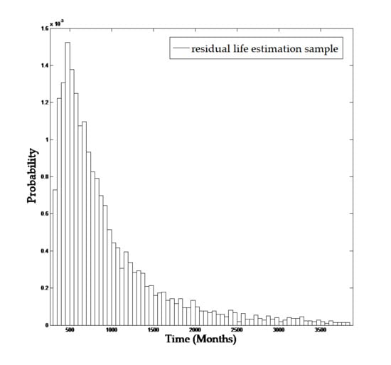
Under the non-informative prior distribution, the point estimation of residual life is 177.5 months. All of them pass the consistency test and can be fused. The sample of residual life drawn by the sample-based method is depicted in Figure 1.

Bayesian estimation and 95% CI results of the residual life by fusing multi-source information are 533.44 months and [91.87, 1220.79] months, respectively. Compared with the previous results [52], the effectiveness and the accuracy of the proposed method are validated. By comparing the weights of multi-source information, the lifetime predicted by the degradation data and expert information provides more reliability information because the historical lifetime dataset is extremely small and zero-failure.

7. Conclusions

In this paper, a Bayesian method is proposed to estimate the residual life of Weibull-distributed components of on-orbit satellites by fusing multi-source information. The contributions of this paper were concluded as follows:

(i).

By fusing prior information, including historical lifetime data, degradation data, similar data and expert information, a more precise estimation of residual life is produced. Both the Bayesian estimate and credible interval are considered in this paper.

(ii).

The Monte Carlo simulation validated the accuracy of the method. The results proved that the Bayesian approach provided more satisfactory and robust estimates than MLE, especially when the sample size of the lifetime data was small. The precision can be improved by fusing multi-source reliability information.

(iii).

The momentum wheel of an on-orbit satellite was taken as an example. The applicability and flexibility of the proposed method were illustrated in the case study. The results were in agreement with those of the simulation study.

This method can be applied to many problems of survival time prediction, and will be of interest to readers in many applications. To extend our research, we think that various kinds of expert information, including point estimation and the CI of the lifetime, merits further research.

References

1. Coro, A.; Abasolo, M.; Aguirrebeitia, J.; De Lacalle, L.L. Inspection scheduling based on reliability updating of gas turbine welded structures. Adv. Mech. Eng. 2019, 11, 1–20. [Google Scholar] [CrossRef]
2. Zhang, Y.; Jia, X.; Guo, B. Bayesian framework for satellite rechargeable lithium battery synthesizing bivariate degradation and lifetime data. J. Cent. South Univ. 2018, 25, 418–431. [Google Scholar] [CrossRef]
3. Zhang, A.; Wang, H.L.; Li, S.B.; Cui, Y.X.; Liu, Z.H.; Yang, G.C.; Hu, J.J. Tansfer learning with deep recurrent neural networks for remaining useful life estimation. Appl. Sci. 2018, 8, 2416. [Google Scholar] [CrossRef]
4. Can, O.; Melin, S.C. Statistical analysis of wind speed using two-parameter Weibull distribution in Alaçatı region. Energy Convers. Manag. 2016, 121, 49–54. [Google Scholar]
5. Ferreira, L.A.; Silva, J.L. Parameter estimation for Weibull distribution with right censored data using EM algorithm. Ekspolatacja Niezawodn.-Maint. Reliab. 2017, 19, 310–315. [Google Scholar] [CrossRef]
6. Bokde, N.; Feijóo, A.; Villanueva, D. Wind Turbine Power Curves Based on the Weibull Cumulative Distribution Function. Appl. Sci. 2018, 8, 1757. [Google Scholar] [CrossRef]
7. Yalcinkaya, M.; Birgoren, B. Confidence interval estimation of Weibull lower percentiles in small samples via Bayesian inference. J. Eur. Ceram. Soc. 2017, 37, 2983–2990. [Google Scholar] [CrossRef]
8. Compare, M.; Baraldi, P.; Bani, I.; Zio, E.; Mc Donnell, D. Development of a Bayesian multi-state degradation model for up-to-date reliability estimations of working industrial components. Reliab. Eng. Syst. Saf. 2017, 166, 25–40. [Google Scholar] [CrossRef]
9. Wang, J.; Huang, H. Road network safety evaluation using Bayesian hierarchical joint model. Accid. Anal. Prev. 2016, 90, 152–158. [Google Scholar] [CrossRef]
10. Mil, S.; Piantanakulchai, M.; Soknath, M.; Mongkut, P. Modified Bayesian data fusion model for travel time estimation considering spurious data and traffic conditions. Appl. Soft Comput. 2018, 72, 65–78. [Google Scholar] [CrossRef]
11. Yang, L.; He, K.; Du, Y.; Guo, Y.; Wang, P. Reliability Analysis to a Satellite-Equipped Harmonic Gear Drive Subjected to Multisource Data and Imbalanced Information. Int. J. Aerosp. Eng. 2018, 2018, 4256302. [Google Scholar] [CrossRef]
12. Bhuyan, P.; Sengupta, D. Estimation of reliability with semi-parametric modeling of degradation. Comput. Stat. Data Anal. 2017, 115, 172–185. [Google Scholar] [CrossRef]
13. Bae, S.J.; Yuan, T.; Kim, S.-J. Bayesian degradation modeling for reliability prediction of organic light-emitting diodes. J. Comput. Sci. 2016, 17, 117–125. [Google Scholar] [CrossRef]
14. Liu, S.; Chen, H.; Guo, B.; Jia, X.; Qi, J. Residual Life Estimation by Fusing Few Failure Lifetime and Degradation Data from Real-Time Updating. In Proceedings of the 2017 IEEE International Conference on Software Quality, Reliability and Security Companion (QRS-C), Prague, Czech Republic, 25–29 July 2017; pp. 177–184. [Google Scholar]
15. Li, Z.; Deng, Y.; Mastrangelo, C. Model selection for degradation-based Bayesian reliability analysis. J. Manuf. Syst. 2015, 37, 72–82. [Google Scholar] [CrossRef]
16. Wang, L.; Pan, R.; Wang, X.; Fan, W.; Xuan, J. A Bayesian reliability evaluation method with different types of data from multiple sources. Reliab. Eng. Syst. Saf. 2017, 167, 128–135. [Google Scholar] [CrossRef]
17. Wang, X.L.; Guo, B.; Cheng, Z.J. Reliability assessment of products with Wiener process degradation by fusing multiple information. Acta Electron. Sin. 2012, 40, 977–982. [Google Scholar]
18. He, D.J.; Wang, Y.P.; Chang, G.S. Objective Bayesian analysis for the accelerated degradation model based on the inverse Gaussian process. Appl. Math. Model. 2018, 61, 341–350. [Google Scholar] [CrossRef]
19. Cheng, Y.; Lu, C.; Li, T.; Tao, L. Residual lifetime prediction for lithium-ion battery based on functional principal component analysis and Bayesian approach. Energy 2015, 90, 1983–1993. [Google Scholar] [CrossRef]
20. Chen, J.Q.; Wang, Y.; Liu, C.H. Empirical Bayes estimation for linear Exponential distribution with contaminated data. Math. Appl. 2018, 31, 949–957. [Google Scholar]
21. Tao, B. On linear empirical Bayes estimation. J. Syst. Sci. Math. Sci. 1986, 6, 195–203. [Google Scholar]
22. Jiang, P.; Xing, Y.; Cheng, W.; Guo, B. An Introduction to Reliability Engineering, 1st ed.; National Defense Industry Press: Beijing, China, 2015; pp. 52–62. [Google Scholar]
23. Zhang, J.; Tang, X. Empirical Bayes Methods for Controlling the False Discovery Rate with Dependent Data; National University of Defense Technology: Changsha, China, 1989. [Google Scholar]
24. Cai, Z.Y.; Cheng, Y.X.; Li, S.L.; Xiang, C.H.; Wang, Z.Z. Residual lifetime prediction method with random degradation and information fusion. J. Shanghai Jiaotong Univ. 2016, 50, 341–350. [Google Scholar]
25. Barraza, N.R. A Parametric Empirical Bayes Model to Predict Software Reliability Growth. Procedia Comput. Sci. 2015, 62, 360–369. [Google Scholar] [CrossRef] [Green Version]
26. Han, L.; Jiang, P.; Yu, Y.; Guo, B. Bayesian reliability evaluation for customized products with zero-failure data under small sample size. In Proceedings of the 2014 International Conference on Reliability, Maintainability and Safety (ICRMS), Guangzhou, China, 6–8 August 2014; pp. 904–907. [Google Scholar]
27. Zhang, Y.; Chen, H.; Jiang, P.; Guo, B. Bayesian assessment for reliability of binomial Components based on information fusion of similar products. J. Donghua Univ. 2015, 32, 940–945. [Google Scholar]
28. Zhang, X.; Mahadevan, S.; Deng, X. Reliability analysis with linguistic data: An evidential network approach. Reliab. Eng. Syst. Saf. 2017, 162, 111–121. [Google Scholar] [CrossRef]
29. Schuh, P.; Stern, H.; Tracht, K. Integration of Expert Judgment into Remaining Useful Lifetime Prediction of Components. Procedia CIRP 2014, 22, 109–114. [Google Scholar] [CrossRef] [Green Version]
30. Yang, Z.; Kan, Y.; Chen, F.; Xu, B.; Chen, C.; Yang, C. Bayesian reliability modeling and assessment solution for NC machine tools under small-sample data. Chin. J. Mech. Eng. 2015, 28, 1229–1239. [Google Scholar] [CrossRef]
31. Guo, J.; Li, Z.J.; Jin, J.H. System reliability assessment with multilevel information using the Bayesian melding method. Reliab. Eng. Syst. Saf. 2018, 170, 146–158. [Google Scholar] [CrossRef]
32. Walter, G.; Flapper, S.D. Condition-based maintenance for complex systems based on current component status and Bayesian updating of component reliability. Reliab. Eng. Syst. Saf. 2017, 168, 227–239. [Google Scholar] [CrossRef] [Green Version]
33. Zhang, J.H. Accuracy detection method using Bayesian multi-sensor data fusing technique. J. Natl. Univ. Def. Technol. 2001, 23, 93–97. [Google Scholar]
34. Feng, J.; Liu, Q.; Zhou, J.L.; Dong, C. Correlation information fusion method and application in reliability analysis. Syst. Eng. Electron. 2003, 25, 682–684. [Google Scholar]
35. Feng, J.; Dong, C.; Liu, Q.; Zhou, J.L. Fusion of information from multiple sources based on adequacy measure in Bayesian analysis. Mini-Micro Syst. 2004, 25, 1356–1358. [Google Scholar]
36. Liu, Q.; Feng, J.; Zhou, J.L. The fusion method for prior distribution based on expert’s information. Chin. Space Sci. Technol. 2004, 24, 68–71. [Google Scholar] [CrossRef]
37. Feng, J.; Liu, Q.; Zhou, J.L.; Dong, C. Multi-Source information fusion based on MEMM in Bayes analysis. Qual. Reliab. 2003, 6, 31–34. [Google Scholar]
38. Feng, J.; Zhou, J.L. Small-Sample reliability information fusion approach based on Bayes-Fuzzy logistic operator. J. Aerosp. Power 2008, 23, 1633–1636. [Google Scholar]
39. Chai, J.; Shi, Y.M.; Wei, J.Q.; Li, X.C. The fusion method for prior distribution in multi-sources of prior information. Sci. Technol. Eng. 2005, 5, 1479–1481. [Google Scholar]
40. Sun, J.; Li, G.L.; Xu, C.; Wang, H.Q. Multi-source information fusion method before test based on ML-II Theory. Comput. Digit. Eng. 2014, 292, 217–219. [Google Scholar]
41. Peng, W.; Xiao, Z.; Wang, Y.; Huang, H.-Z.; Liu, Y. A combined Bayesian framework for satellite reliability estimation. In Proceedings of the 2011 International Conference on Quality, Reliability, Risk, Maintenance, and Safety Engineering, Xi’an, China, 17–19 June 2011; pp. 13–21. [Google Scholar]
42. Peng, W.; Huang, H.-Z.; Xie, M.; Yang, Y.; Liu, Y. A Bayesian Approach for System Reliability Analysis with Multilevel Pass-Fail, Lifetime and Degradation Data Sets. IEEE Trans. Reliab. 2013, 62, 689–699. [Google Scholar] [CrossRef]
43. Han, L. Research on Reliability Assessment methods for Satellite Platform Based on Multi-source Information Fusion. Master’s Thesis, National University of Defense Technology, Changsha, China, November 2014; pp. 36–38. [Google Scholar]
44. Liu, B.Y.; Wang, J.Q. Compatibility Check of the Prior Information on Low Voltage Switchgear. Appl. Mech. Mater. 2013, 330, 830–833. [Google Scholar] [CrossRef]
45. Akram, M.; Hayat, A. Comparison of Estimators of the Weibull Distribution. J. Stat. Theory Pract. 2014, 8, 238–259. [Google Scholar] [CrossRef]
46. Guo, J.; Li, Z.J.; Keyser, T. A Bayesian approach for integrating multilevel priors and data for aerospace system reliability assessment. Chin. J. Aeronaut. 2014, 31, 41–53. [Google Scholar] [CrossRef]
47. Hastings, W.K.; Mardia, K.V. Monte Carlo Sampling Methods Using Markov Chains and Their Applications. Biometrika 1970, 57, 97–109. [Google Scholar] [CrossRef]
48. Wang, C.; Lu, N.; Wang, S.; Cheng, Y.; Jiang, B. Dynamic Long Short-Term Memory Neural-Network- Based Indirect Remaining-Useful-Life Prognosis for Satellite Lithium-Ion Battery. Appl. Sci. 2018, 8, 2078. [Google Scholar] [CrossRef]
49. Li, M.; Zhang, X. Information Fusion in a Multi-Source Incomplete Information System Based on Information Entropy. Entropy 2017, 19, 570. [Google Scholar] [CrossRef]
50. Cheng, Y.H.; Tian, J.; Lu, N.Y.; Jiang, B. Research on life prediction of momentum wheels system based on DTBN. Aerosp. Control 2016, 34, 89–94. [Google Scholar]
51. Li, H.T.; Jin, G.; Zhou, J.L.; Zhou, Z.B.; Wu, C.H. Momentum wheel Wiener process degradation modeling and life prediction. J. Aerosp. Power 2011, 26, 622–627. [Google Scholar]
52. Liu, Q.; Huang, X.P.; Zhou, J.L.; Jin, G.; Sun, Q. Failure physics-analysis-based method of Bayesian reliability estimation for momentum wheel. Acta Aeronaut. Astronaut. Sin. 2009, 30, 1392–1397. [Google Scholar]
Figure 1. Residual life estimation sample drawn by the sample-based method.
Applsci 09 03017 g001