Article

Real-Time Automated Segmentation and Classification of Calcaneal Fractures in CT Images

1
Department of Electrical Engineering, National Central University, Zhongli 32001, Taiwan
2
Department of Computer Science and Electronics, Universitas Gadjah Mada, Yogyakarta 55281, Indonesia
*
Author to whom correspondence should be addressed.
Appl. Sci. 2019, 9(15), 3011; https://doi.org/10.3390/app9153011
Submission received: 14 June 2019 / Revised: 17 July 2019 / Accepted: 23 July 2019 / Published: 26 July 2019
(This article belongs to the Special Issue Intelligent Processing on Image and Optical Information)

Abstract

:

Featured Application

Segmentation and classification of calcaneal fractures.

Abstract

Calcaneal fractures often occur because of accidents during exercise or activities. In general, the detection of the calcaneal fracture is still carried out manually through CT image observation, and as a result, there is a lack of precision in the analysis. This paper proposes a computer-aid method for the calcaneal fracture detection to acquire a faster and more detailed observation. First, the anatomical plane orientation of the tarsal bone in the input image is selected to determine the location of the calcaneus. Then, several fragments of the calcaneus image are detected and marked by color segmentation. The Sanders system is used to classify fractures in transverse and coronal images into four types, based on the number of fragments. In sagittal image, fractures are classified into three types based on the involvement of the fracture area. The experimental results show that the proposed method achieves a high precision rate of 86%, with a fast computational performance of 133 frames per second (fps), used to analyze the severity of injury to the calcaneus. The results in the test image are validated based on the assessment and evaluation carried out by the physician on the reference datasets.

1. Introduction

The calcaneus is the largest tarsal bone that has the responsibility of supporting the axial load of the body’s weight [1]. A calcaneal fracture is the most common in the tarsal bone fractures, most of which are intra-articular fractures, which usually occur as a result of falling from a height, sports injuries, and vehicle accident [2]. The severity of fracture displacement and the extent of soft tissue injury are directly related to the amount of energy absorbed by the limbs in producing injury [3]. Injuries with higher energies produces soft tissue disorders that are more severe and may cause open fractures [4]. Bleeding fractures into the plane of the fascial, which surrounds the heel, produce severe pain above the fracture and may result in a leg compartment syndrome [5]. Furthermore, calcaneal fractures have presented a significant challenge for orthopedic surgeons in patients’ treatment [6,7]. So, detection of the calcaneal fracture is an important subject for patient diagnostic decisions and treatment planning [8,9].
Modern calcaneal fracture classification systems rely on three-dimensional computed tomography (CT) rather than two-dimensional conventional radiography [10]. Although a CT image contains a significant amount of medical information, it is not accurate enough to examine fractures through manual visual inspection due to its low resolution [11]. Thus, details, such as the skeletal structures, the boundary between internal organs and bone, and soft tissue in the bone may not be accurately seen and assessed depending on the experience of the physician [12]. Therefore, a computer-aided method for fracture detection is needed which can significantly assist physicians to examine CT images, and it is crucial for physicians to make diagnostic decisions, as well as plan treatments, based on this information [13]. In addition, with a computer-aid, faster and more detailed fracture detection can be achieved.
Recently, several approaches have been proposed to detect bone fractures in CT images of various areas of the human body. Wu et al. [14] proposed a method for automatic fracture detection of CT images of traumatic pelvic injuries. These fractures are detected using a segmentation technique, which consists of four main parts: Pre-processing, edge detection, shape matching, and Registered Active Shape Model (RASM) with an automatic initialization. However, this segmentation method only applies to the reference frame, which was generated based on previously known pelvic bone anatomy information. Roth et al. [15] implemented a method for the automatic detection of posterior element fractures on spinal CT images. This method used the multi-atlas label fusion to segment the spinal vertebral body and computed the edge map of its posterior elements. But, this segmentation region is predicted on the set of probabilities for fractures along the edges of the image, which are limited to the spine. These aforementioned works [14,15] show that a computer-aided method provides more accurate results for fracture detection and has the potential to accelerate the assessment of trauma cases, reduce the possibility of misclassification of bone fractures, and reduce variability between observers. But, these methods cannot be applied to the calcaneus bones, which have different shapes, features, and types of fracture than their study. In the case of the calcaneus, segmentation and detection of the calcaneal fracture are very challenging, due to the low resolution of CT images, the complex anatomy, and soft tissue structures of the calcaneus [16,17]. At present, there are deficiencies in the operative or conservative management planning of the calcaneus, which are caused by the lack of a standard system in the classification of calcaneal fractures [18].
A study to apply image processing for the detection and classification of calcaneal fractures has not been widely performed. Pranata et al. [19] has proposed automated classification and detection of calcaneus bone fracture locations in CT images. This method classifies the calcaneal fractures into two classes: Fractured and non-fractured. However, the classification results do not provide more detailed conclusions about the fractures type of each anatomical plane orientation, where the identification of fracture alone is not sufficient to assess injury severity. Moreover, the orientation of the calcaneus anatomical plane is manually registered and the computation time is 5 min and 10 s, which are not fast enough for real-time applications.
In this paper, a new method for the automated segmentation and detection of calcaneal fractures for real-time applications is proposed. The main objective is to provide results for calcaneus segmentation and detection of fractures for each anatomical plane orientation, so that physicians can better, and further assess fractures in the calcaneus region with a shorter processing time. One of the challenges in detecting calcaneal fractures is the different shape of the calcaneus in each patient’s CT image [10,11,12]. As such, the shape approach cannot be used to find the calcaneus based on its shape in the tarsal bone. Furthermore, due to limited features and colors in the CT images, it is a difficult task to identify calcaneus in the tarsal bone. To solve this problem, the region of interest (ROI) of the calcaneus is determined based on the anatomical plane orientation of the tarsal bones, i.e., transverse, coronal, and sagittal. In addition, due to quality limitations in CT images, it is a challenging task to classify the type of fracture for calcaneus. In particular, mild and small fractures, that only appear slightly in CT images, cannot be detected a physician at first inspection because the physician may not be able to reliably call them to rely on these fractures, due to the quality of CT and the amount of data to be processed [14,15]. Thus, for fractures that appear slightly in CT images, repeated inspections are required to identify the existence and details of the fracture. Computer-based analyses can be used to process detailed information from several neighboring slices to give instructions to the physician on whether a particular slice contains a fracture, then details of the separation between pieces can be identified [12,14] can be extracted. However, due to the anatomical variability between individuals, the accuracy in segmentation and detection of fractures in the calcaneus structure remain a challenging task. This proposed method provides the calcaneus segmentation to show the details of the fractures in the calcaneus region, which can be fragments or lines. This method has performed the segmentation by detecting the calcaneus bone structure, based on the white bone area on the CT images. Then, the fracture type is classified based on the amount of the fragments and the location of the lines fractures.
The remainder of this paper is organized as follows. Section 2 introduces a literature review of the classification of calcaneal fractures and describes the main algorithm. Section 3 illustrates the performance of fracture detection results in CT images. Finally, conclusions are drawn in Section 4.

2. Materials and Methods
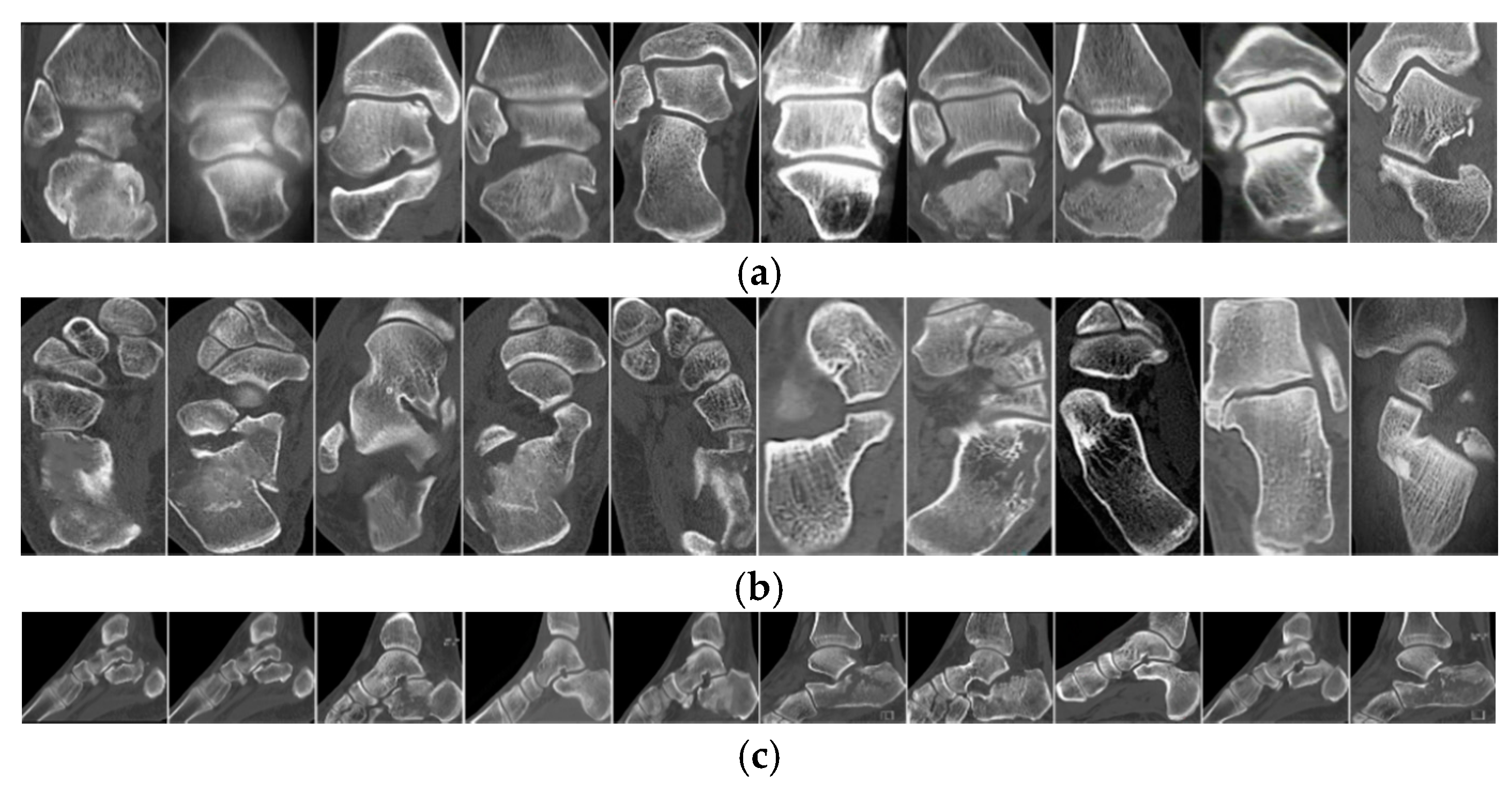
2.1. Materials

We obtained 2210 CT Digital Imaging and Communications in Medicine (DICOM) images from the datasets with assessment and evaluation of the fracture type information [1,2,3,4,5,6,7,8,9,10,11,12,13], radiopedia (https://radiopaedia.org/), anesthesia key (https://aneskey.com/fractures-and-dislocations-of-the-tarsal-bones/), and CT images from two patients with three anatomical plane orientations. The dataset consists of 815 coronal images, 777 transverse images, and 618 sagittal images. The experiment was conducted using Visual Studio C++ 2017 in the 3.40 GHz CPU with 8 GB RAM.

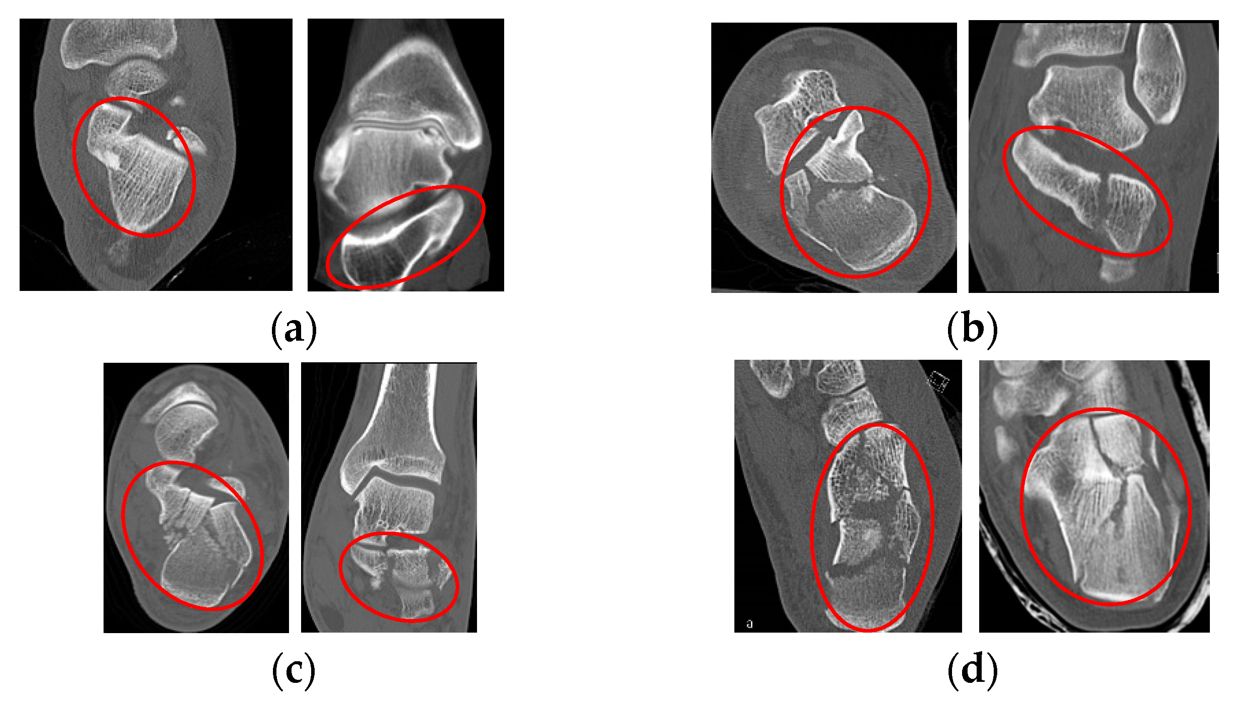
2.2. Fractures Classification in Calcaneus

On the basis of subtalar joint involvement, calcaneal fractures observed in CT images have been divided into two categories: Intra-articular and extra-articular. Intra-articular is a fracture involving the joints, including damage to the connective tissue between two bones. Extra-articular is a fracture that does not involve the joints, rather, it includes pieces of bone drawn from the calcaneus by the ligament.
The intra-articular fractures of the calcaneus represent about 75% of all calcaneal fractures in adults [1,2], where the prospect of recovery depends on how severely the calcaneus was damaged during injury. Several classification systems for intra-articular fractures of the calcaneus have been developed, in which the Sanders system [20,21] is the most commonly used due to its correlation with clinical outcomes and lower inter-observer variability [22]. This classification divides the intra-articular fractures into four types, based on the number of fragments in the calcaneus, i.e., Type I, Type II, Type III, and Type IV.
Figure 1 shows examples of calcaneal fractures on the transverse and coronal planes, the red circle shows the location of the calcaneus in the tarsal structure. Type I is a non-displaced extra-articular fracture with a displacement of less than 2 mm; this is also knowns as a line fracture. Types II–IV are displaced intra-articular fractures corresponding to an increase in the number of fragments, in which Type IV has more than three fragments.
Extra-articular fractures represent about 25% of calcaneal fractures and include all fractures that do not involve the posterior aspect of the subtalar joint [1,8]. Extra-articular fractures are normally caused by trauma, such as a crush or mild injury. Based on the location of the fracture, several methods [1,10,12] classify extra-articular fractures of the calcaneus into three types, i.e., Type A, Type B, and Type C. Figure 2 shows an example of fractures on the sagittal plane. The red circle shows the location of the calcaneal fractures in sagittal images. The Type A fracture involves the anterior process of the calcaneus (Figure 2b). The Type B fracture extends through the calcaneus or middle calcaneus, including the lateral processes (Figure 2c); and the Type C fracture is a calcaneal fracture involving the posterior (Figure 2d).

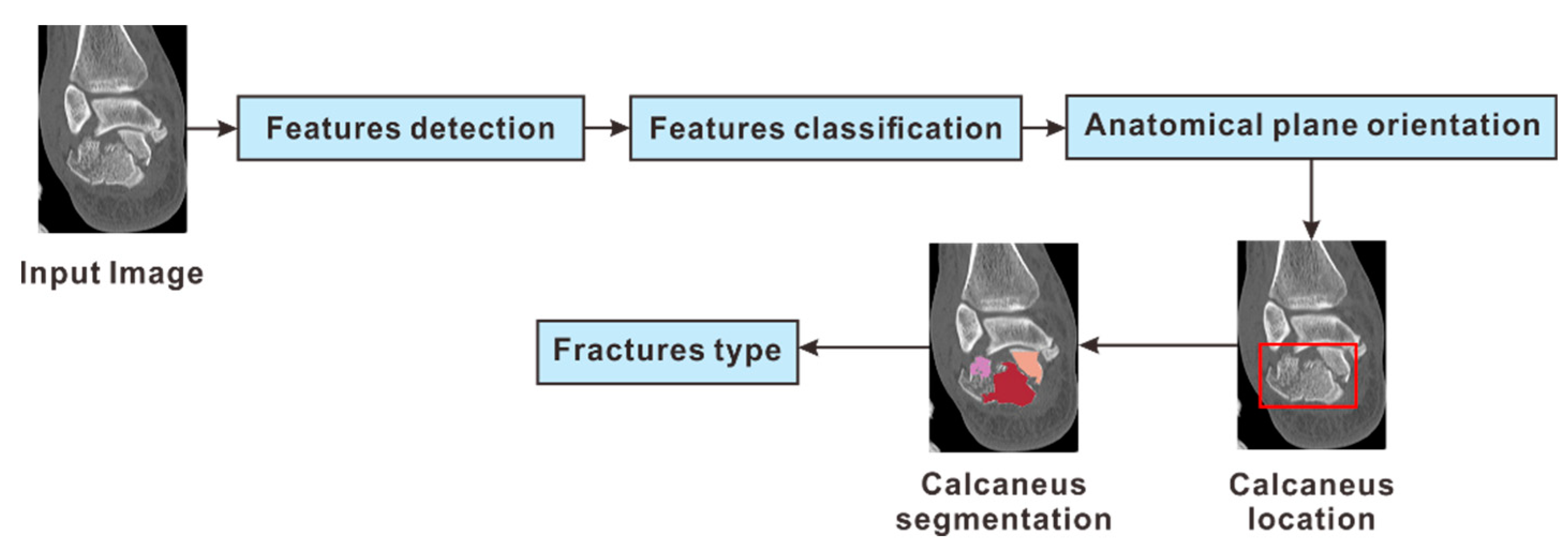
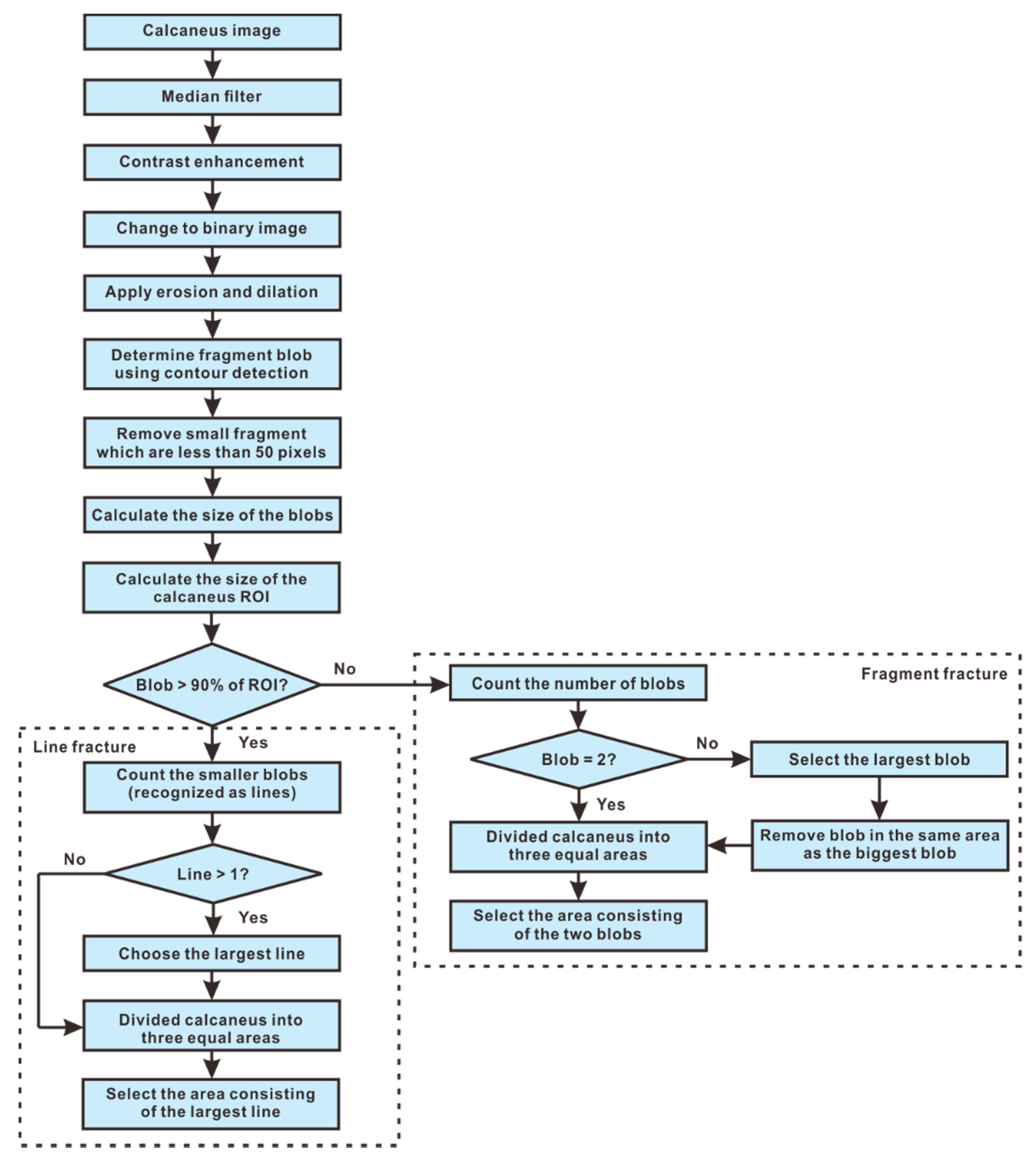
2.3. System Overview

Figure 3 shows a general overview of the system proposed in this paper. The algorithm contains two steps to complete the main task: Step 1 involves the detection of the calcaneus location in the input image using a machine learning approach; and Step 2 involves the segmentation of the calcaneus ROI, based on several morphology methods, and contour detection of the fragmented region so as to determine the type of calcaneal fracture.

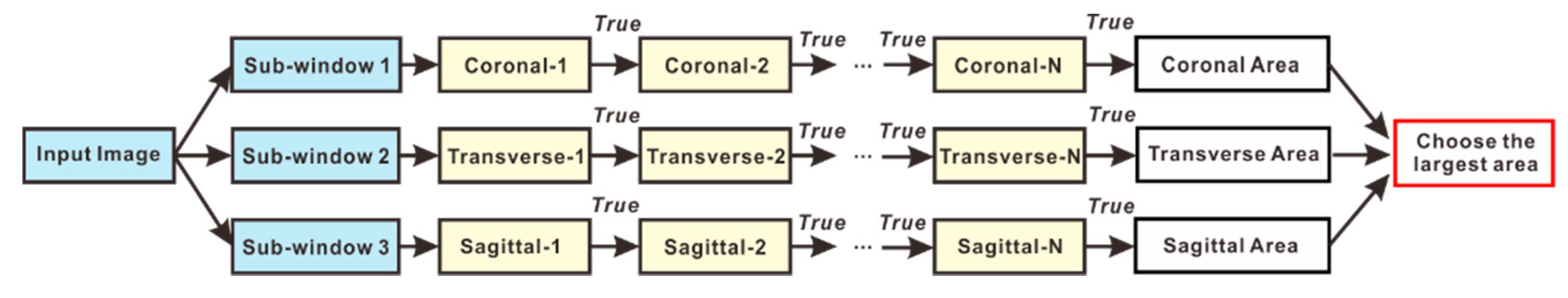
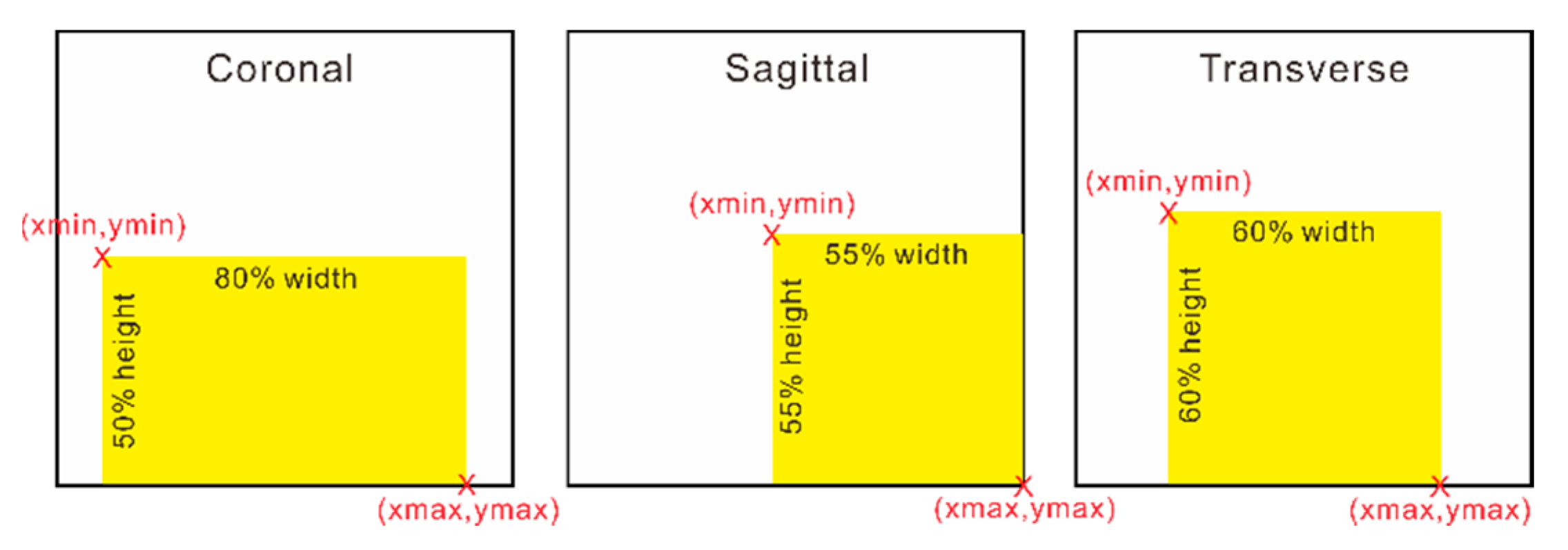
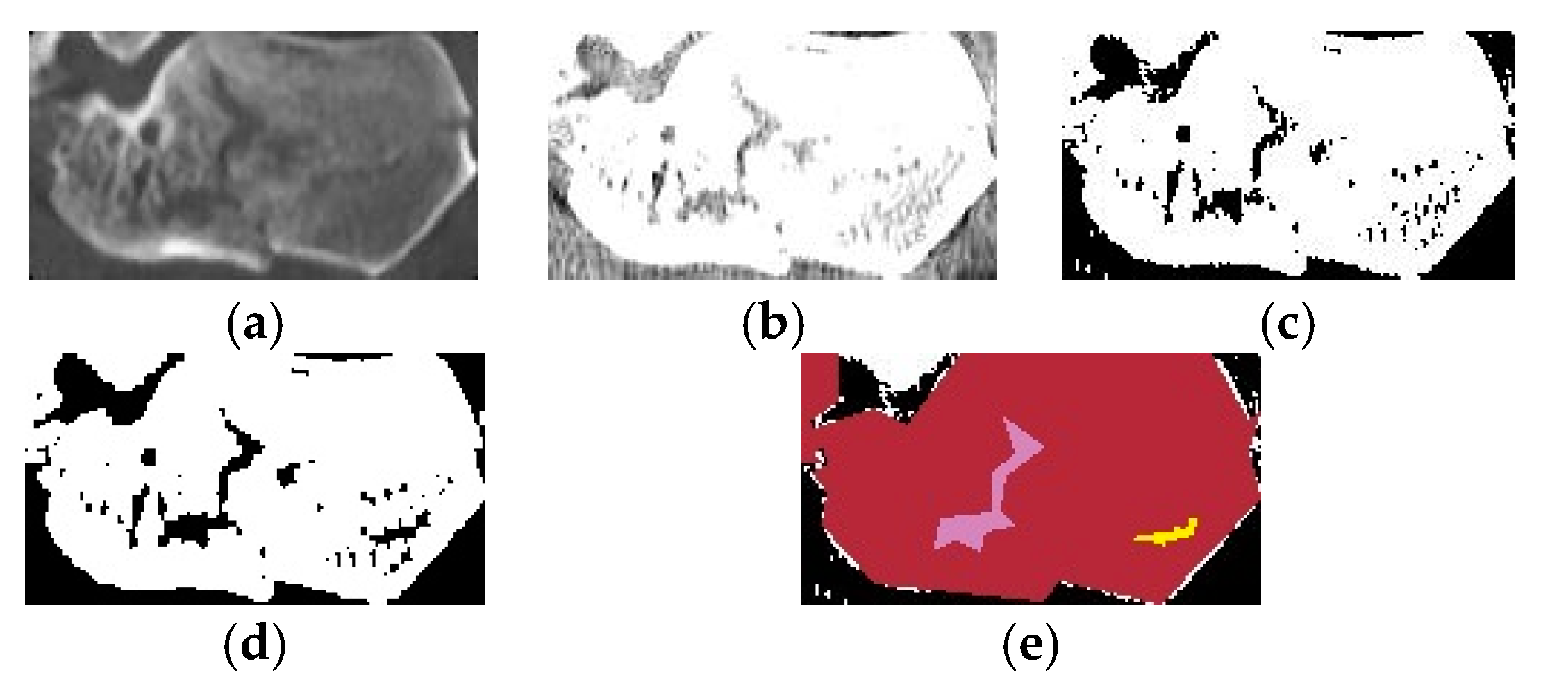
2.4. Step 1: Detection of Calcaneus Location

In the first step, the extended local binary pattern (LBP) [23] and cascade classifier [24] are used to determine the anatomical plane orientation in the input image based on the shape of the tarsal bone. The basic idea behind LBP is that the image is composed of a micro-pattern. LBP is the first-order circular derivative pattern generated by concatenating the direction of the binary gradient. CT scans are generally available as DICOM files, where each image contains a 2D array with pixel intensity. The CT DICOM image is a grayscale image in which the bone area is represented by white pixels surrounded by gray pixels. Therefore, LBP is suitable for defining the information in CT DICOM images, based on texture descriptors.
The LBP operator is the sum of the gray-level intensities label computed at each pixel location. The LBP code labels can be expressed as:
L B P ( S , R ) = S = 0 S 1 b ( g ) 2 S
where g = g s g c , S is the number of pixels in a small circular neighborhood with radius R (R can be the value within 1–3, in this study we set R = 1), g s is the grey-level intensities label of S, g c is the grey-level intensity of the center pixel, and the function b(g) is defined as:
b ( g ) = { 1 ,   if   g 0 0 ,   otherwise .
The LBP code label histogram contains information about edge distribution and other local features in the image, so it can be used to describe the image texture in the CT DICOM image. The LBP feature is extracted from the input image at the pixel location (i,j). Then, the image is divided into several small non-overlapping blocks to get the feature histogram. The region blocks Ak are the same size, where k = 0 , , K and K is the number of blocks in the image. The LBP histogram of the labeled image is defined as:
H ( L ) = ( i , j ) A k h ( i , j ) ( l )
where h ( i , j ) ( l ) is the value of the bin l which consists of a look-up table of 29-1 = 511 bins, l is the LBP feature computed at location (i,j) and L is the number of different labels produced by the LBP operator. Figure 4 shows the process that is used to provide three types of information: Code labels for local textures, histograms in local regions, and feature histograms whereby the tarsal bone structure in each anatomical plane orientation is described. The feature histogram is the concatenation of each region histogram into a single LBP histogram.
In this step, the AdaBoost algorithm [25,26] is used to select the features of the classifier in the training stage. The classifier is selected to evaluate a single LBP histogram which maximizes the margin between positive and negative samples. The classifier determines the best threshold classification function for each histogram so that the number of misclassified instances can be minimized. The negative image input of each anatomical plane is the orientation of the other plane. In the training stages, the features in positive and negative images will be learned as positive, and negative labels, respectively. Figure 5 shows the example images for training, which are the tarsal bone shape in each anatomical plane of various sizes of input images. In this study, the images used have minimum and maximum sizes of 126 × 147, and 980 × 1024, respectively.
A training sample is set as ( x m , y m ) , m = 1 , 2 , , M , where y m = 0 ,   or   1 for negative, or positive labels, respectively, is the class label for the sample x m . Firstly, the initial weight vector is set as ω 1 ( m ) = 1 / M . The classifier is defined as λ n ( x m ) = 0 ,   or   1 where n = 1 , 2 , , N is the iteration number. The error associated with the classifier is evaluated as:
ε n = m = 1 M ω n ( m ) ,   if   | λ n ( x m ) y m | .
The selected classifier is used to update the weight vector as:
ω n + 1 ( m ) = ω n ( s ) β n 1 τ m   where   τ m = { 0 ,   if   x m   classified   correctly 1 ,   otherwise
and β n is the weighting parameter computed from:
β n = ε n 1 ε n
The result of the training stage is the labeled result of each region which is represented as:
W ( x ) = { 1 ,   if   n = 1 N [ λ n ( x ) × log ( 1 β n ) ] 1 2 n = 1 N log ( 1 β n ) 0 ,   otherwise .
In the testing stages, the shape of the tarsal bones is detected by the sliding window method [24], in which each sub-window contains labels for each anatomical plane orientation from the training stage. Each area, which passes by each sub-window, is labeled at each classification stage either as, positive (1) or negative (0). If the label detected is positive, the region is recognized as the object and the classifier passes to the next stage. Otherwise, the region is rejected immediately. Then, the last stage will show the result of the detector in the current window, as shown in Figure 6. If there is more than one anatomical plane orientation detected in the input image, then the largest area of the current window is selected. The location of the calcaneus, based on the selected anatomical plane orientation, is determined according to Figure 7. Then, the calcaneus ROI is used as the location of the input image for the next step.

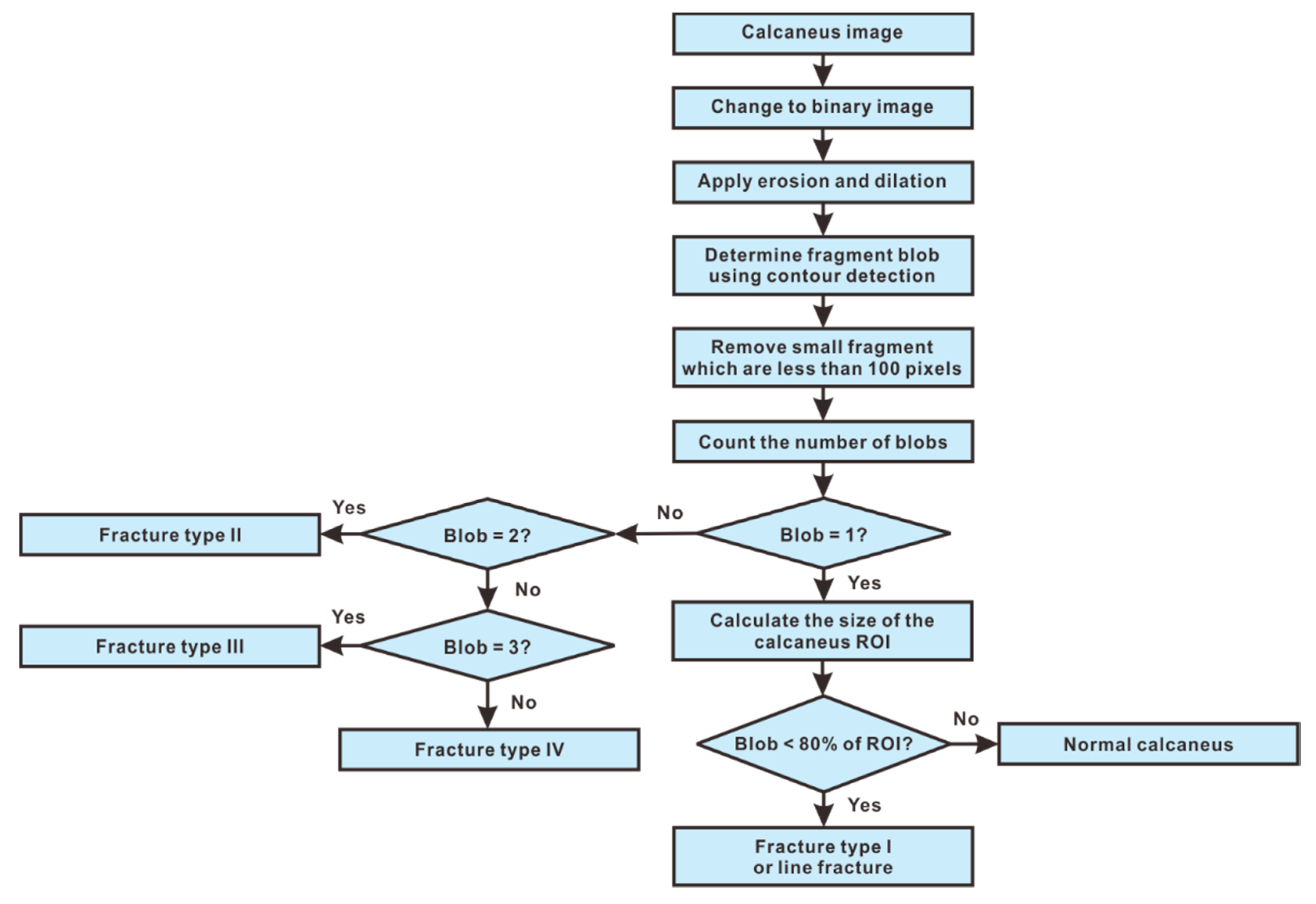
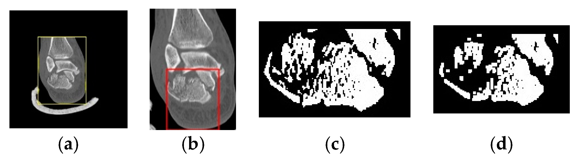
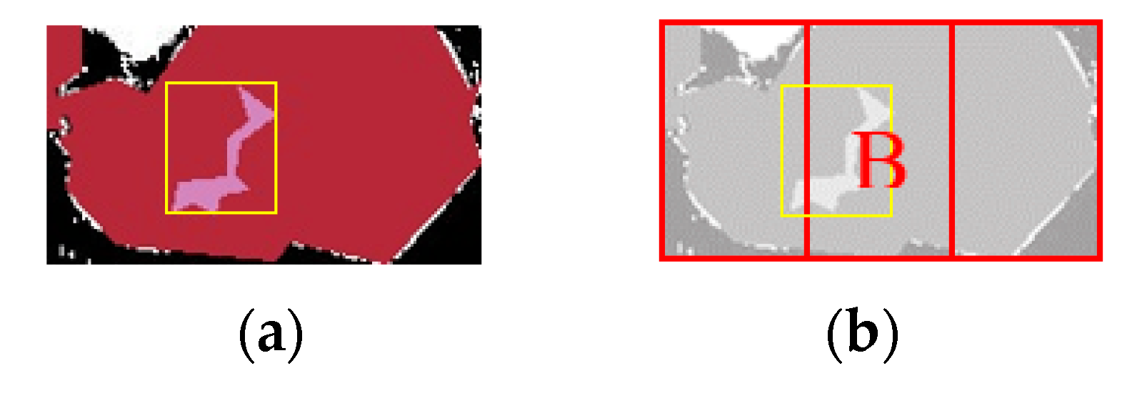
2.5. Step 2: Segmentation of the Calcaneus Fragments

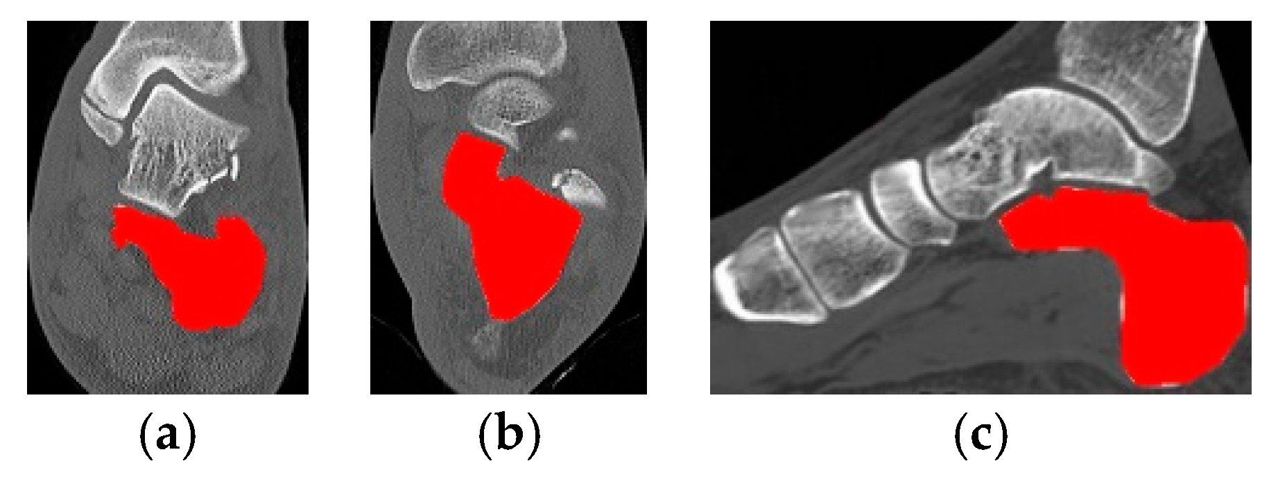
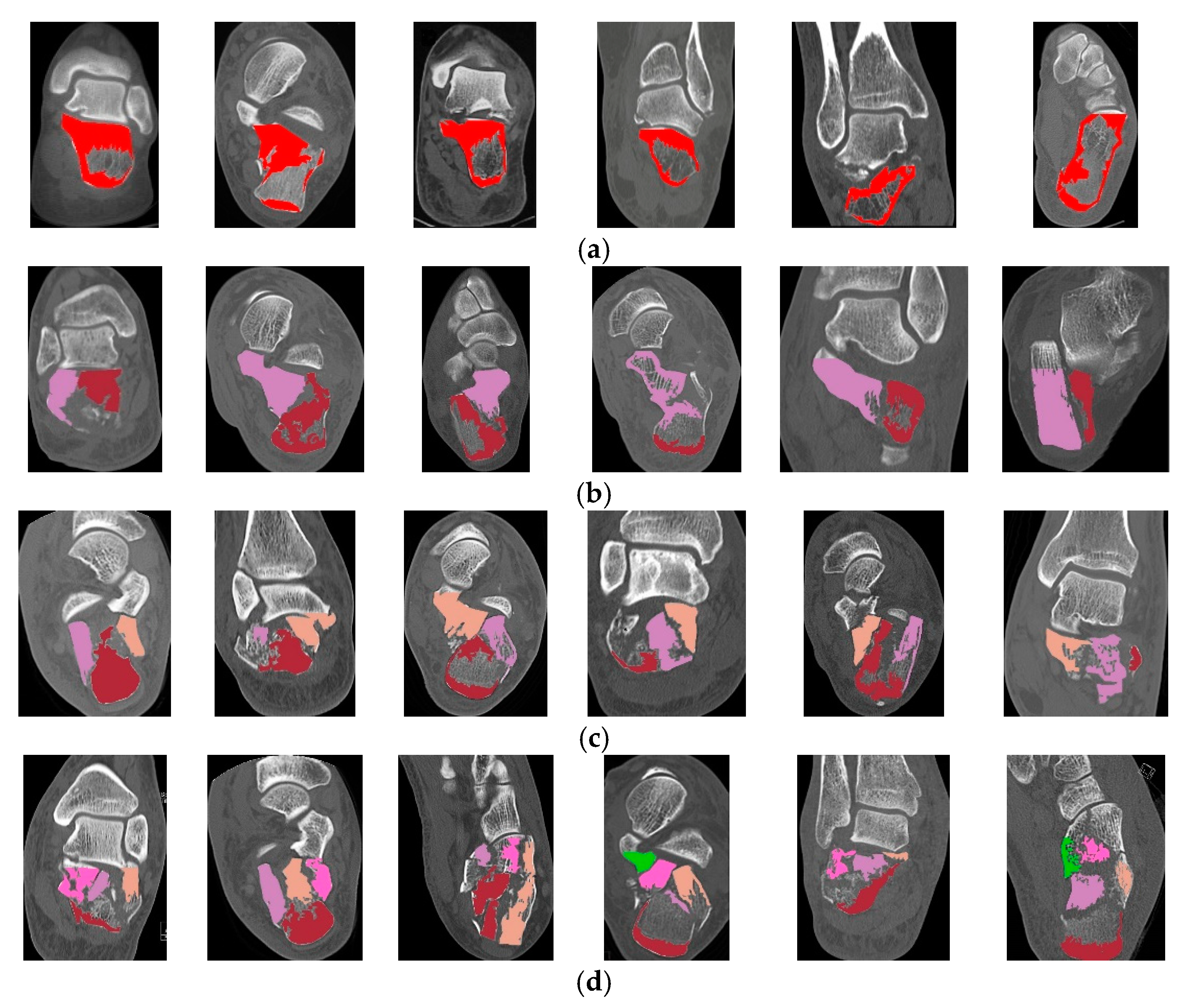
2.5.1. Classification of Calcaneal Fractures in Coronal and Transverse Images

In the next step, the regional segmentation method, based on the contour detection [27], is applied to determine the type of fracture. Figure 8 shows the steps for determining the type of calcaneal fracture in coronal and transverse images.
Figure 9a shows the selected tarsal bone region using LBP features and cascade classifier. Figure 9b shows the location of the calcaneus determined in accordance with Figure 7 (see Section 2.4). Several morphological operations are applied in the calcaneus region to separate the fractional area. Figure 9c shows the calcaneus region having been converted into a binary image using Otsu segmentation [28]. This step selects a threshold to minimize the intra-class variance in black (background) and white (foreground) pixels. Then, the automatic threshold selection is used to segment the image. The optimal threshold selection is based on thresholds that minimize within-class weighted variance [28] which is equivalent to maximizing the intra-class variance.
For each given threshold intra-class variance can be computed by
σ B 2 ( z ) = q b ( z ) ( 1 q b ( z ) ) ( μ b ( z ) μ f ( z ) ) 2
where z = 1 , 2 , , 256 is the gray level of the input calcaneus image, μ b and μ f are the means of background and foreground, respectively, which are defined as:
μ b ( z ) = i = 0 z 1 i × P ( i ) q b ( z )
μ f ( z ) = i = z E 1 i × P ( i ) q f ( z )
where E is the bins of the histogram, q b ( z ) = i = 0 z 1 P ( i ) and q f ( z ) = i = z E 1 P ( i ) are the gray level probability distributions P ( i ) for the background, and foreground, respectively. Then, the optimum threshold is obtained by maximizing the between-class variances.
T h = arg ( max 1 z < 256 σ B 2 ( z ) ) .
Figure 9d shows the erosion and dilation morphological operations [29], which are implemented on binary images. The erosion filter removes white pixels along the foreground boundaries in the form of fragments of the calcaneus, so that the value of neighboring pixels in the foreground becomes minimum. Dilation adds white pixels to the foreground boundaries in the image so that the neighboring pixels in the foreground can have a maximum value.

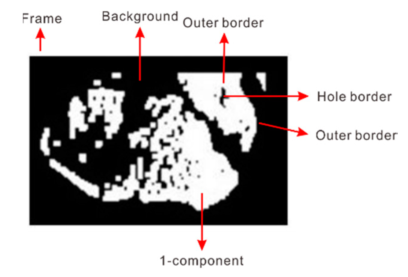
2.5.2. Contour Detection

The final step is to use the contour detection algorithm to extract regional boundaries in a calcaneal fracture. The initial value is set to 1 to determine the affiliation of the new contours and other contours. The outer border is the boundary with white pixels (1-component) which are enclosed by the black pixels (0-component). The hole border is the 1-component boundary which is enclosed by the 0-component. The frame is the boundary of the image that is wrapped by 1-component. NBD is the number of contours in the current calculation. LNBD is the last border number encountered when scanning a starting point. Figure 10 shows the connected components and borders in the image.
The sub-steps for detection of contour of the calcaneus ROI are as follows:
1. Find the starting point of the contour
Start from the upper-left pixel at location (0,0) of the calcaneus ROI, then the image is scanned row-by-row. This condition indicates that the outer contour that has not been passed as the pixel value is changed in the next contour. Values greater than 1 indicates an 8-connected case that can represent the hole contours that have not been passed.
2. Contour Following
Next, start from the starting point that obtained from the previous step. Then the image is scanned row by row and the edges of 1-component is recorded. The square-tracing algorithm [30] is used since it is suitable for 4-connected cases as follows:
  • If the current pixel value is 1, change the scan direction to the left and move 1 pixel. Conversely, when the pixel value is 0, change the scan direction to the right and move 1 pixel.
  • Continue sub-steps 2a until the current contour point returns to the starting point.
The outer contour is the contour that passes through the entire contour in different directions. Then, change the pixel value in the following contour procedure. If the neighboring point (p + 1, q) of the current contour point (p, q) has a pixel value of 0, set the current point to –NBD. In addition, if the current point value is more than 1 NBD, it remains unchanged. Otherwise, it is set to NBD.
Algorithm 1: Build Contour Hierarchies.
S = corresponding LNDB
S’ = new contour found
If S = OUTER and S’ = OUTER
 If S = HOLE and S’ = HOLE
  Build the same hierarchy parent for S and S’
  Add S to the last of children linked list of S’
 Else
  Let S’ be the parent of S
  If SS’S child = 0
   Let S to be the first child of S’
  Else
   Add S to the last of children linked list of S’
  End
 End
End
3. Build Contour Hierarchies
The next sub-step is to find out the relationship between contours. NBD that hits the contour during step 1 will be scanned and recorded in LNBD. Each boundary extracted is stored as a point vector which is retrieved and reconstructed with a full hierarchy of nested contours. Then, each contour is encoded with four points. The result is a closed two-dimensional contour for each remaining region as shown in Figure 11a. The contour boundary is a dense set of sequential neighbor points called a blob. A blob larger than 100 pixels is selected and the minimum closing circle is found so that each blob represents one fragment as shown in Figure 11b. The algorithm is shown as follows:
In transverse and coronal images, if the calcaneus is segmented into a single full blob then it is classified as a normal calcaneus. If the calcaneus is detected as one blob but the area is not full, it is classified as type I (line fracture). Otherwise, the type of fracture is classified by a number of blobs.

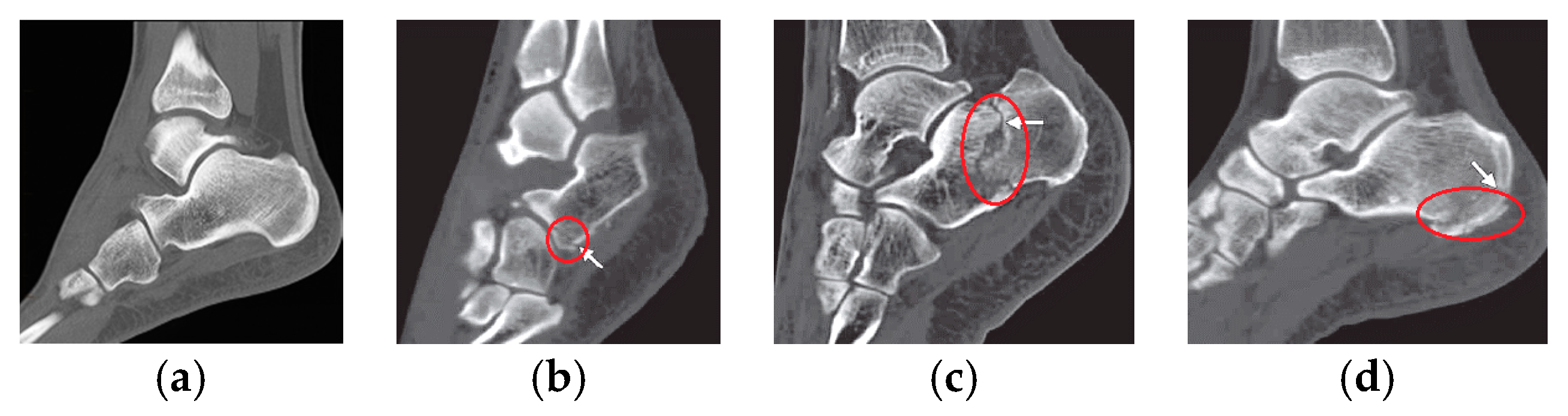
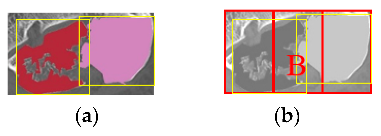
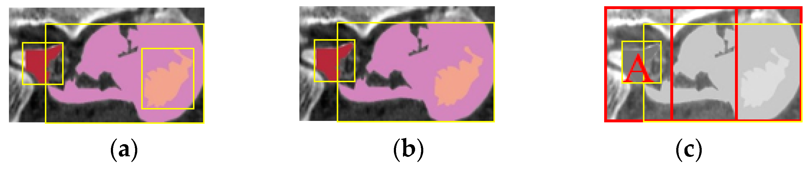
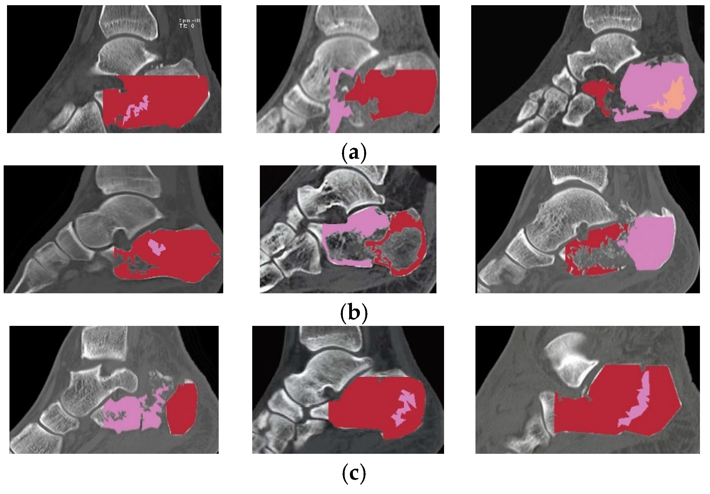
2.5.3. Classification of Calcaneal Fractures in Sagittal Images

Figure 12 defines the steps for determining the type of calcaneal fracture in sagittal images. The calcaneus region is divided into three equal areas where each area represents an extra-articular region: Type A (left), Type B (middle), and Type C (right). The fracture classification in sagittal image is based on the area of the fracture line. However, it is slightly difficult to separate the lines from the bone structure. Thus, the median filter [31] is applied to reduce the ambiguity between a bone structure and fracture, as shown in Figure 13a. Then, the automatic contrast enhancement [32] is implemented to obtain a clear fragment separation in bone structure, as shown in Figure 13b. The image histogram, which shows the relationship between the gray level and the corresponding frequency, can be expressed as:
I h i s t ( z ) = Δ z Δ
where Δ z is the number of pixels in z, and Δ is the total number of pixels in the input image. The histogram equalization (HE) accumulates a histogram of the pixel values in the input image, then displaces all pixel values to enhance the contrast. HE with interval [ 0 , D 1 ] can be computed by:
M a p z = F ( j ) = ( D 1 ) z = 1 j 1 I h i s t ( z )
where Mapz indicates an F(j) mapping function that maps every pixel value j from the input image to Mapz, and D is the dynamic range of HE in the output image.
Figure 13c shows the Otsu segmentation, which is implemented to convert Figure 13b into a binary image. Figure 13d shows the erosion and dilation which makes the fracture line more obvious. Figure 13e shows the fracture lines and fragmented areas using a contour detection algorithm (see Section 2.5.2). The largest blob is selected as the calcaneus region and other blobs can be recognized as fractures. Figure 13e indicates that there is more than one fracture line detected in the calcaneus region. Then, the largest line is selected to determine the type of fracture, based on the line position in the calcaneus body, as shown in Figure 14a.
Figure 14a indicates the area of the selected fracture line. In Figure 14b, the calcaneal fracture is classified as Type B, since most of the area of the fracture is in the middle region. In the case of fragments, the region of each fragment is selected, as shown in Figure 15a. Figure 15b shows the fracture type (called Type B in the middle region), which is determined by the area between the two fragments.
Figure 16 shows another case of fragment detection. Figure 16a shows the area of two fragments detected in the same region. Since the smaller fragment is inside the larger fragmented region, only the largest fragment will be selected as shown in Figure 16. Figure 16c indicates this calcaneal fracture is classified as Type A, since the left area consists of two fragmented regions.

3. Experimental Results and Discussion

Figure 17 and Figure 18a show the calcaneus classified as non-fracture and Type I, in which both have one segmented region, represented by only one color of the calcaneus segmentation. In non-fractured calcaneus images, the calcaneus region may be fully segmented. In Type I fracture images, the calcaneus region cannot be fully segmented, as there are several fracture lines in the calcaneus body.
Figure 18 shows each color on the calcaneus segmentation representing one fragment. Although the type of fracture can be determined based on the number of fragments, the location of the fragments in the calcaneus is different with different shapes. In images of Type II fractures, failure of segmentation results will cause errors in the detection of fracture types. Thus, the calcaneus will be detected as a Type III fracture. This is due to the ambiguity in the bone structure that causes errors in separating a single blob into two blobs. In images of Type III fractures, failure of segmentation results will cause errors in detecting two blobs as a single blob. This is due to the ambiguity of the CT image, which makes the algorithm unable to separate the white pixels between the two fragments.
Due to several factors mentioned, the most accurate detection results relate to Type IV fracture images. Since Type IV fractures have more than three fragments, some errors in the segmentation results do not significantly affect the detection of fracture types, which are determined by the number of fragments.
Table 1 shows the accuracy of fracture detection in coronal and transverse images. In coronal images, fragment separation is shown more clearly than in the transverse images. In transverse images, the bone structure is slightly ambiguous, thus making segmentation fail to separate the foreground (bone structure) and background. If the segmentation fails, the fragment region cannot be filled as a single blob and it will be considered as an additional fragment. The proposed method achieves an average accuracy of 87.25% for coronal images and 83.25% for transverse images.
Figure 19 shows the fracture segmentation results in sagittal images. Table 2 shows the accuracy of the fracture type detection in sagittal images. In sagittal images, fractures in the calcaneus region are too ambiguous and almost similar to the bone structure. Common mistakes in fracture detection in sagittal image are as follows:
  • Bone structure is detected as a fracture,
  • The fracture in the image is too similar to the bone structure, so it is not recognized as a fracture.
The most accurate results in sagittal image is for Type B fractures, where the area of the fracture is located in the middle of the calcaneus. In images with type A (left) and type C (right) fractures, the fracture line is too vague within the bone structure, so that some errors occur in the segmentation result. The proposed method achieves an average accuracy of 82% for sagittal images. Thus, the average accuracy performance for fracture type detection in the calcaneus is 84.17%.
The results of computation performance are summarized in Table 3 in respect of frames per second (fps). The average time cost is about 7.5 ms per frame or 133 fps. The fastest processing time is for sagittal images that have the smallest calcaneus region, compared to other anatomical planes. The slowest processing time is for coronal images, which have the largest calcaneus region. The part that uses the greatest cost in computational time is segmentation so that the size of the calcaneus region determines the processing speed of a CT image.
Table 4 shows the performance accuracy in terms of True Positive (TP), False Positive (FP), False Negative (FN), Precision Rate (PR), recall, and F-measure, based on the classification results, which are indicated in the segmented area. This performance result is checked for each image manually. TP is the detected area corresponds to the associated fracture. FP is the detected area not related to the fracture. FN is the area associated with a fracture which is not detected. The accuracy of the performance can be computed by:
P R = T P T P + F P
Recall = T P T P + F N
F-measure = 2 × P R × Recall P R + Recall
The proposed method achieves an average precision rate of 0.86 and recall of 0.89. The highest recall is 0.92 for coronal images that have a clearer separation between the bone structure on the calcaneus, and the background compared to transverse and sagittal images. The sagittal image has the lowest recall caused by ambiguity on the fracture line with the bone structure.

4. Conclusions

This paper presents a new method in automatically segmenting and detecting calcaneal fractures in CT images in real time applications. As shown in the result, the proposed algorithm in detecting the calcaneal fractures is relatively accurate. Using the proposed algorithm, bone fractures can be further highlighted in the processed images. This can help physicians to analyze the CT images better and increase the possibility of getting the real fracture condition. In addition, the method designed by us can estimate the distance of fracture separation and the angle between broken bone pieces, as well as other quantitative fracture assessments, which may not be easily accessed and measured through visual inspection. The proposed algorithm provides an analysis guide to fracture detection automatically with fast processing of more than one hundred images in one second. Thus, this method can help physicians to reduce decision-making and diagnostic time, which is very important for traumatic calcaneus injury.

Author Contributions

W.R. contributed to the conception of the study and wrote the manuscript; performed the experiment and data analyses; and contributed significantly to algorithm design and manuscript preparation; W.-J.W. helped perform the analysis and contribute to constructive discussions.

Funding

This research received no external funding.

Conflicts of Interest

The authors declare no conflict of interest.

References

  1. Badillo, K.; Pacheco, J.A.; Padua, S.O.; Gomez, A.A.; Colon, E.; Vidal, J.A. Multidetector CT evaluation of calcaneal fractures. Radiographics 2011, 31, 81–92. [Google Scholar] [CrossRef] [PubMed]
  2. Swanson, S.A.; Clare, M.P.; Sanders, R.W. Management of Intra-Articular Fractures of the Calcaneus. Foot Ankle Clin. 2008, 13, 659–678. [Google Scholar] [CrossRef] [PubMed]
  3. Rammelt, S.; Zwipp, H. Calcaneus fractures: Facts, controversies and recent developments. Injury 2004, 35, 443–461. [Google Scholar] [CrossRef] [PubMed]
  4. Park, C.H.; Lee, D.Y. Surgical treatment of sanders type 2 calcaneal fractures using a sinus tarsi approach. Indian J. Orthop. 2017, 51, 461–467. [Google Scholar] [CrossRef] [PubMed]
  5. Feng, Y.; Shui, X.; Ying, X.; Cai, L.; Yu, Y.; Hong, J. Closed Reduction and Percutaneous Fixation of Calcaneal Fractures in Children. Orthopedics 2016, 39, e744–e748. [Google Scholar] [CrossRef] [PubMed]
  6. Hoelscher-Doht, S.; Frey, S.P.; Kiesel, S.; Meffert, R.H.; Jansen, H. Subtalar Dislocation: Long-Term Follow-Up and CT-Morphology. Open J. Orthop. 2015, 5, 53–59. [Google Scholar] [CrossRef] [Green Version]
  7. Mostafa, M.F.; El-Adl, G.; Hassanin, E.Y.; Abdellatif, M.S. Surgical treatment of displaced intra-articular calcaneal fracture using a single small lateral approach. Strat. Trauma Limb Reconstr. 2010, 5, 87–95. [Google Scholar] [CrossRef] [Green Version]
  8. Rammelt, S.; Godoy-Santos, A.L.; Schneiders, W.; Fitze, G.; Zwipp, H. Foot and ankle fractures during childhood: Review of the literature and scientific evidence for appropriate treatment. Rev. Bras. Ortop. 2016, 51, 630–639. [Google Scholar] [CrossRef]
  9. Dhillon, M.S.; Prabhakar, S. Treatment of displaced intra-articular calcaneus fractures: A current concepts review. SICOT-J 2017, 3, 59. [Google Scholar] [CrossRef]
  10. Moussa, K.M.; Hassaan, M.A.E.; Moharram, A.N.; Elmahdi, M.D. The role of multidetector CT in evaluation of calcaneal fractures. Egypt. J. Radiol. Nucl. Med. 2015, 46, 413–421. [Google Scholar] [CrossRef] [Green Version]
  11. Daftary, A.; Haims, A.H.; Baumgaertner, M.R. Fractures of the Calcaneus: A Review with Emphasis on CT. Radiographics 2005, 25, 1215–1226. [Google Scholar] [CrossRef] [PubMed]
  12. Galluzzo, M.; Greco, F.; Pietragalla, M.; De Renzis, A.; Carbone, M.; Zappia, M.; Maggialetti, N.; D’andrea, A.; Caracchini, G.; Miele, V. Calcaneal fractures: Radiological and CT evaluation and classification systems. Acta Biomed. 2018, 89, 138–150. [Google Scholar] [PubMed]
  13. Harnroongroj, T.; Suntharapa, T.; Arunakul, M. The new intra-articular calcaneal fracture classification system in term of sustentacular fragment configurations and incorporation of posterior calcaneal facet fractures with fracture components of the calcaneal body. Acta Orthop. Traumatol. Turc. 2016, 50, 519–526. [Google Scholar] [CrossRef] [PubMed] [Green Version]
  14. Wu, J.; Davuluri, P.; Ward, K.R.; Cockrell, C.; Hobson, R.; Najarian, K. Fracture Detection in Traumatic Pelvic CT Images. Int. J. Biomed. Imaging 2012, 2012, 1–10. [Google Scholar] [CrossRef] [PubMed]
  15. Roth, H.R.; Wang, Y.; Yao, J.; Lu, L.; Burns, J.E.; Summers, R.M. Deep convolutional networks for automated detection of posterior-element fractures on spine CT. Med. Imaging 2016 Comput. Aided Diagn. 2016, 9785, 97850. [Google Scholar]
  16. Long, C.; Fang, Y.; Huang, F.G.; Zhang, H.; Wang, G.L.; Yang, T.F.; Liu, L. Sanders II–III calcaneal fractures fixed with locking plate in elderly patients. Chin. J. Traumatol. 2016, 19, 164–167. [Google Scholar] [CrossRef] [PubMed]
  17. Biz, C.; Barison, E.; Ruggieri, P.; Iacobellis, C. Radiographic and functional outcomes after displaced intra-articular calcaneal fractures: A comparative cohort study among the traditional open technique (ORIF) and percutaneous surgical procedures (PS). J. Orthop. Surg. Res. 2016, 11, 92. [Google Scholar] [CrossRef] [PubMed]
  18. Dhillon, M.S.; Bali, K.; Prabhakar, S. Controversies in calcaneus fracture management: A systematic review of the literature. Musculoskelet. Surg. 2011, 95, 171–181. [Google Scholar] [CrossRef]
  19. Pranata, Y.D.; Wang, K.C.; Wang, J.C.; Idram, I.; Lai, J.Y.; Liu, J.W.; Hsieh, I.H. Deep learning and SURF for automated classification and detection of calcaneus fractures in CT images. Comput. Methods Programs Biomed. 2019, 171, 27–37. [Google Scholar] [CrossRef]
  20. Sanders, R.; Fortin, P.; DiPasquale, T.; Walling, A. Operative treatment in 120 displaced intraarticular calcaneal fractures. Results using a prognostic computed tomography scan classification. Clin. Orthop. Relat. Res. 1993, 290, 87–95. [Google Scholar]
  21. Sanders, R. Displaced Intra-Articular Fractures of the Calcaneus. J. Bone Jt. Surg. Am. 2000, 82, 225–250. [Google Scholar] [CrossRef] [PubMed]
  22. Janzen, D.L.; Connell, D.G.; Munk, P.L.; E Buckley, R.; Meek, R.N.; Schechter, M.T. Intraarticular fractures of the calcaneus: Value of CT findings in determining prognosis. Am. J. Roentgenol. 1992, 158, 1271–1274. [Google Scholar] [CrossRef] [PubMed]
  23. Huang, D.; Shan, C.; Ardabilian, M.; Wang, Y.; Chen, L. Local Binary Patterns and its application to facial image analysis: A Survey. IEEE Trans. Syst. Man Cybern. Part C 2011, 41, 765–781. [Google Scholar] [CrossRef]
  24. Ludwig, O.; Nunes, U.J.C.; Ribeiro, B.; Premebida, C. Improving the generalization capacity of cascade classifiers. IEEE Trans. Cybern. 2013, 43, 2135–2146. [Google Scholar] [CrossRef] [PubMed]
  25. Yu, H.; Moulin, P. Regularized Adaboost learning for identification of time-varying content. IEEE Trans. Inf. Forensics Secur. 2014, 9, 1606–1616. [Google Scholar] [CrossRef]
  26. Viola, P.; Jones, M.J. Robust real-time object detection. Int. J. Comput. Vis. 2004, 57, 137–154. [Google Scholar] [CrossRef]
  27. Suzuki, S.; Be, K. Topological structural analysis of digitized binary images by border following. Comput. Vis. Graph. Image Process. 1985, 30, 32–46. [Google Scholar] [CrossRef]
  28. Yang, X.; Shen, X.; Long, J.; Chen, H. An improved median-based otsu image thresholding algorithm. AASRI Procedia 2012, 3, 468–473. [Google Scholar] [CrossRef]
  29. Gonzalez, R.C.; Woods, R.E. Digital Image Processing; Prentice Hall: Upper Saddle River, NJ, USA, 2002; ISBN 0201180758. [Google Scholar]
  30. Seo, J.; Chae, S.; Shim, J.; Kim, D.; Cheong, C.; Han, T.D. Fast Contour-Tracing Algorithm Based on a Pixel-Following Method for Image Sensors. Sensors 2016, 16, 353. [Google Scholar] [CrossRef]
  31. Zhu, Y.; Huang, C. An Improved Median Filtering Algorithm for Image Noise Reduction. Phys. Procedia 2012, 25, 609–616. [Google Scholar] [CrossRef] [Green Version]
  32. Chen, C.M.; Chen, C.C.; Wu, M.C.; Horng, G.; Wu, H.C.; Hsueh, S.H.; Ho, H.Y. Automatic Contrast Enhancement of Brain MR Images Using Hierarchical Correlation Histogram Analysis. J. Med. Biol. Eng. 2015, 35, 724–734. [Google Scholar] [CrossRef] [PubMed] [Green Version]
Figure 1. The Sanders system of fracture classification on the calcaneus [1,2,20]: (a) Normal calcaneus in transverse and coronal images; (b) Type II; (c) Type III; and (d) Type IV.
Applsci 09 03011 g001
Figure 2. Classification of calcaneus fractures in sagittal images [1,8,10]: (a) Normal calcaneus; (b) Type A; (c) Type B; and (d) Type C.
Applsci 09 03011 g002
Figure 3. System overview of the proposed method.
Applsci 09 03011 g003
Figure 4. Input image region.
Applsci 09 03011 g004
Figure 5. Example images of the tarsal bone: (a) Coronal; (b) Transverse; and (c) Sagittal.
Applsci 09 03011 g005
Figure 6. Cascade classifier stage to select anatomical plane orientation.
Applsci 09 03011 g006
Figure 7. Region of interest (ROI) of the calcaneus based on the anatomical plane orientation.
Applsci 09 03011 g007
Figure 8. Algorithm for determining the type of calcaneal fracture in the coronal and transverse image.
Applsci 09 03011 g008
Figure 9. (a) Tarsal bone detection; (b) Calcaneus region; (c) Binary image of calcaneus region; and (d) Calcaneus region after morphological operations.
Applsci 09 03011 g009
Figure 10. Connected components and borders.
Applsci 09 03011 g010
Figure 11. Fragment segmentation: (a) Contour detection and (b) Color segmentation.
Applsci 09 03011 g011
Figure 12. Algorithm for determining the type of calcaneal fracture in sagittal images.
Applsci 09 03011 g012
Figure 13. (a) Apply median filter; (b) Contrast enhancement; (c) Otsu segmentation; (d) Morphological operations; and (e) Fracture detection.
Applsci 09 03011 g013
Figure 14. Steps to determine the type of fracture in case of a line fracture: (a) The region of the fracture line is represented by a yellow box and (b) The fracture type is based on the line region.
Applsci 09 03011 g014
Figure 15. Steps to determine the type of fracture in case of fragment fracture: (a) The region of the fragment is represented by a yellow box and (b) The fracture type is based on the area between the two fragments.
Applsci 09 03011 g015
Figure 16. (a) Two fragments are in the same region; (b) The largest fragment is selected; and (c) The fracture type is based on the area between these two fragments.
Applsci 09 03011 g016
Figure 17. Normal calcaneus segmentation: (a) Coronal; (b) Transverse; and (c) Sagittal.
Applsci 09 03011 g017
Figure 18. Segmentation result of the calcaneal fractures based on Sanders classification: (a) Type I; (b) Type II; (c) Type III; and (d) Type IV.
Applsci 09 03011 g018
Figure 19. Segmentation result of the calcaneal fractures in sagittal images: (a) Type A; (b) Type B; and (c) Type C.
Applsci 09 03011 g019
Table 1. Accuracy of the fractures type detection based on Sanders classification.
Fractures TypeCoronal (%)Transverse (%)
Type I8884
Type II8681
Type III8380
Type IV9288
Average87.2583.25
Table 2. Accuracy of the fractures type detection in sagittal image.
Fractures TypeSagittal (%)
Type A81
Type B85
Type C80
Average82
Table 3. Computational performance in fps.
Anatomical PlaneAverage fps
Coronal92.33
Transverse146.67
Sagittal160.33
Table 4. Detection result performance.
Anatomical PlaneTPFPFNPRRecallF-Measure
Coronal921370.870.920.89
Transverse8711100.880.890.88
Sagittal8215120.850.870.86
Average Accuracy87139.60.860.890.8

