Article

Quantitative Analysis of Benign and Malignant Tumors in Histopathology: Predicting Prostate Cancer Grading Using SVM

1
Department of Computer Engineering, u-AHRC, Inje University, Gimhae 50834, Korea
2
Department of Digital Anti-Aging Healthcare, Inje University, Gimhae 50834, Korea
3
Department of Pathology, Yonsei University Hospital, Seoul 03722, Korea
*
Author to whom correspondence should be addressed.
Appl. Sci. 2019, 9(15), 2969; https://doi.org/10.3390/app9152969
Submission received: 12 June 2019 / Revised: 22 July 2019 / Accepted: 22 July 2019 / Published: 24 July 2019
(This article belongs to the Special Issue Texture and Colour in Image Analysis)

Abstract

:
An adenocarcinoma is a type of malignant cancerous tissue that forms from a glandular structure in epithelial tissue. Analyzed stained microscopic biopsy images were used to perform image manipulation and extract significant features for support vector machine (SVM) classification, to predict the Gleason grading of prostate cancer (PCa) based on the morphological features of the cell nucleus and lumen. Histopathology biopsy tissue images were used and categorized into four Gleason grade groups, namely Grade 3, Grade 4, Grade 5, and benign. The first three grades are considered malignant. K-means and watershed algorithms were used for color-based segmentation and separation of overlapping cell nuclei, respectively. In total, 400 images, divided equally among the four groups, were collected for SVM classification. To classify the proposed morphological features, SVM classification based on binary learning was performed using linear and Gaussian classifiers. The prediction model yielded an accuracy of 88.7% for malignant vs. benign, 85.0% for Grade 3 vs. Grade 4, 5, and 92.5% for Grade 4 vs. Grade 5. The SVM, based on biopsy-derived image features, consistently and accurately classified the Gleason grading of prostate cancer. All results are comparatively better than those reported in the literature.

Graphical Abstract

1. Introduction

Prostate adenocarcinoma, a type of prostate cancer, is the second most commonly diagnosed cancer. In the United States, the incidence of prostate cancer ranks first among all malignant tumors in men. The Gleason score is currently the most common grading system of prostate adenocarcinoma and is widely used to assess the prognosis of men with prostate cancer using samples from a prostate biopsy. There are some diagnostic protocols for cancer grading, for which microscopic evaluation of tissue specimens is required. For this, the samples need to be appropriately stained using Hematoxylin and Eosin (H&E) compounds. The cancer grade is assessed by a pathologist based on the morphological features of lumen and cell nucleus observed in the tissue. Cancer diagnosis and grading based on digital pathology have become increasingly complex due to the increase in cancer occurrence and specific treatment options for patients [1].
In South Korea, the incidence of prostate cancer is increasing significantly. Prostate cancer (PCa) is the fifth most common cancer among males in Korea and the expected cancer deaths in 2018 were 82,155 [2]. The detection of prostate cancer has always been a major issue for pathologists and medical practitioners, for both diagnosis and treatment. Usually, the cancer detection process in histopathology consists of categorizing stained microscopic biopsy images into malignant and benign.
The Gleason grade grouping system defines Gleason scores ≤ 6 as grade 1, score 3 + 4 = 7 as grade 2, score 4 + 3 = 7 as grade 3, score 4 + 4 ,   3 + 5   or   5 + 3 = 8 as grade 4, and score 4 + 5 ,   5 + 4   or   5 + 5 = 9   or   10 as grade 5. The Gleason score is obtained by adding the primary (most common) and secondary (second most common) scores from H&E stained tissue microscopic images. This system was developed by Dr. Donald F Gleason, who was a Pathologist in Minnesota, and members of the Veterans Administration Cooperative Urological Research Group (VACURG) [3]. This system was tested on a large number of patients, including long-term follow-ups and is considered an outstanding success.
In recent years, an excellent and important addition to microscopy and digital imaging has been developed for microscopes that are used to convert stained tissue slides into whole slide digital images. This allows for more efficient computer-based viewing and analysis of histopathology. Early diagnosis and treatment are required, to avoid the enlargement of cancer cells in the prostate gland and control the spreading of more aggressive tumors to other parts of the body.
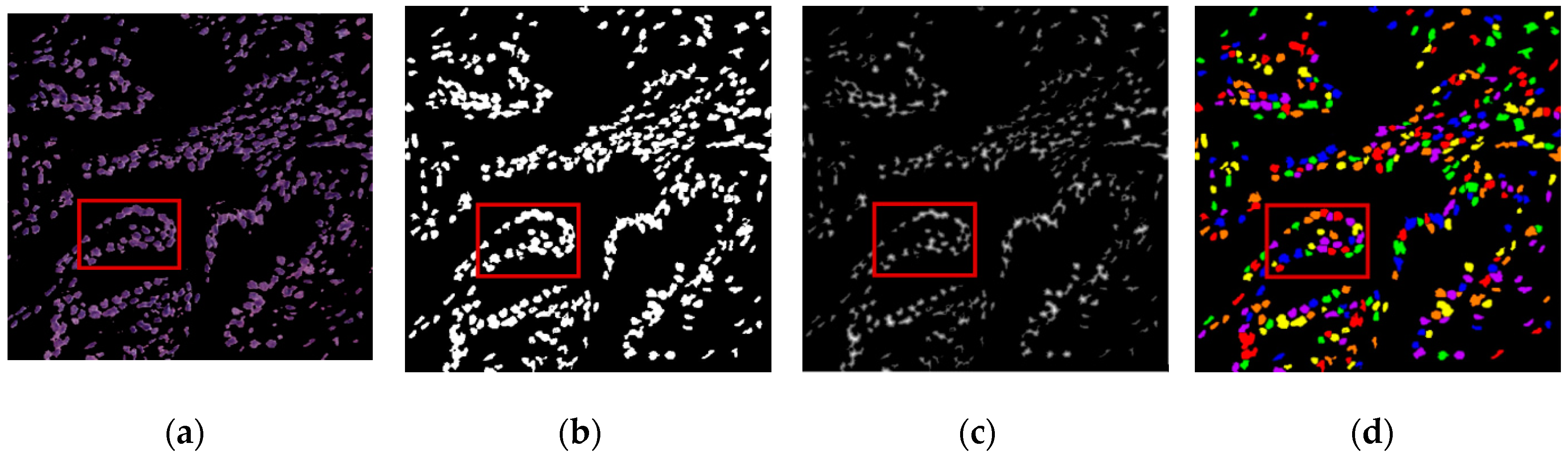
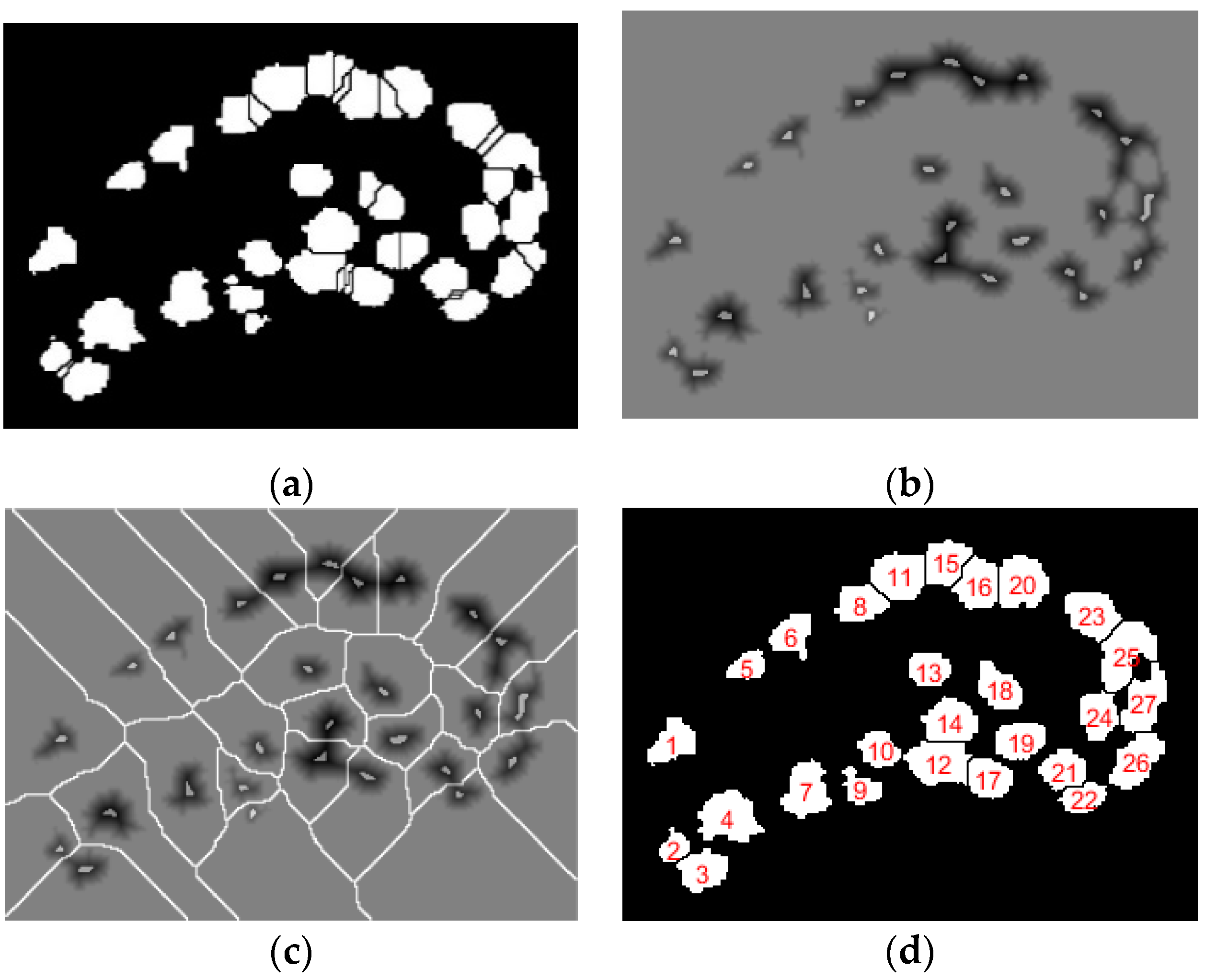
The digital pathology field has grown dramatically over recent years, largely due to technological advancements in image processing and machine learning algorithms, and increases in computational power. As part of this field, many methods have been proposed for automatic histopathological image analysis and classification. In this paper, color segmentation, based on k-means clustering method, is proposed for microscopic biopsy tissue image processing, and the watershed algorithm has been implemented to separate touching cell nuclei in tissue images.
This approach can be implemented in different ways; however, the marker selection approach has been carried out in this study to control over-segmentation. Diagnosing prostate cancer from a biopsy tissue image under a microscope is difficult for the pathologists and doctors. Therefore, machine learning and deep learning techniques are developed for computerized classification and cancer grading. In this study, a machine learning classification method is proposed in order to classify Gleason grade groups of prostate cancer. From a perspective of computer engineering, since the regular procedure of diagnosing prostate cancer and grading is difficult and time consuming; therefore, automated computerized methods are in high demand and are essential for medical image analysis.

2. Literature Review

Tabesh et al. [4] extracted features that describe color, texture, and morphology from 367 and 268 H&E image patches, which were acquired from tissue microarray (TMA) datasets. These features were used for support vector machine (SVM) classification. They achieved an accuracy of 96.7% and 81% for predicting benign vs. malignant and low-grade vs. high-grade classifications, respectively, using 5-fold cross-validation.
Doyle et al. [5] proposed a cascade approach to the multi-class grading problem. They used cascade binary classification to maximize inter- and intra-class accuracy rather than the conventional one-shot classification and one-versus-all approaches to multi-class classification. In the proposed cascade approach, each division is classified separately and independently.
Nir et al. [6] proposed some novel features based on intra- and inter-nuclei properties for classification. They trained their classifier on 333 tissue microarray (TMA) cores annotated by six pathologists for different Gleason grades and used SVM classification to achieve an accuracy of 88.5% and 73.8% for cancer detection (benign vs. malignant) and low vs. high grade (Grade 3 vs. Grade 4, 5), respectively.
Doyle et al. [7] extracted nearly 600 image texture features to perform pixel-wise Bayesian classification at each image scale to obtain the corresponding likelihood scene. The authors achieved an accuracy of 88.0% for distinguishing between benign and malignant samples.
Rundo et al. [8] proposed Fuzzy C-Means (FCM) clustering algorithm for prostate multispectral MRI morphologic data processing and segmentation. The authors used co-registered T1w and T2w MR image series and achieved an average dice similarity coefficient 90.77 ± 7.75, with respect to 81.90 ± 6.49 and 82.55 ± 4.93 by processing T2w and T1w imaging alone, respectively.
Jiao et al. [9] used combined deep learning and SVM methods for breast masses classification. The methods were applied to the Digital Database for Screening Mammography (DDSM) dataset and achieved high accuracy under two objective evaluation measures. The authors used nearly 600 images, out of these, 50% were benign and 50% were malignant. The classification accuracy achieved in this paper was 96.7% for distinguishing between benign and malignant samples.
Hu et al. [10] presented a novel mass detection system for digital mammograms, which integrated a visual saliency model with deep learning techniques. The authors used combined deep learning and SVM methods for image and feature classification, respectively. They achieved an average accuracy of 91.5% in mass detection between cancer and benign datasets.
Naik et al. [11] presented a method for automated histopathology images. They have demonstrated the utility of glandular and nuclear segmentation algorithm in accurate extraction of various morphological and nuclear features for automated grading of prostate cancer, breast cancer, and distinguishing between cancerous and benign breast histology specimen. The authors used a SVM classifier for classification of prostate images containing 16 Gleason grade 3 images, 11 grade 4 images, and 17 benign epithelial images of biopsy tissue. They achieved an accuracy of 95.19% for grade 3 vs. grade 4, 86.35% for grade 3 vs. benign, and 92.90% for grade 4 vs. benign.
Nguyen et al. [12] introduced a novel approach to grade prostate malignancy using digitized histopathological specimens of the prostate tissue. They have extracted tissue structural features from the gland morphology and co-occurrence texture features from 82 regions of interest (ROI) with 620 × 550 pixels to classify a tissue pattern into three major categories: benign, grade 3 carcinoma, and grade 4 carcinoma. The authors proposed a hierarchical (binary) classification scheme and obtained 85.6% accuracy in classifying an input tissue pattern into one of the three classes.
Albashish et al. [13] proposed some texture features, namely Haralick, Histogram of Oriented Gradient (HOG), and run-length matrix, which have been extracted from nuclei and lumen images individually. They used a total of 149 images with 4140 × 3096 pixels, and the dataset was randomly divided into 50% for training and 50% for testing. An ensemble machine learning classification system was proposed, and achieved an accuracy of 88.9% for Grade 3 vs. Grade 4, 92.4% for benign vs. Grade 4, and 97.85% for benign vs. Grade 3. These accuracies were averaged over 50 simulation runs and statistical significance.
Diamond et al. [14] used morphological and texture features to classify the sub-region of 100 × 100 pixels and subjected each to image-processing techniques. They classified a tissue image into either stroma or prostatic carcinoma. In addition, the authors used lumen area to discriminate benign tissue from the other two classes. As a result, 79.3% of sub-regions were correctly classified.
Ding et al. [15] introduced an automated image analysis framework capable of efficiently segmenting microglial cells from histology images and analyzing their morphology. Their experiments show that the proposed framework is accurate and scalable for large datasets. They extracted three types of features for SVM classification, namely Mono-fractal, Multi-fractal, and Gabor features.
Yang et al. [16] used image processing and machine learning algorithms to analyze the smear images captured by the developed image-based cytometer. A low-cost, portable image-based cytometer was built for image acquisition from Giemsa stained blood smear. The authors selected 50 images manually for the training set, out of these, 25 images were parasites and 25 images were non-parasites. The selected images were then segmented separately to extract the features for Support Vector Machine (SVM) classification, and they used linear kernel classifier to train and test these features.

3. Materials and Methods

3.1. Tissue Image Dataset

The histopathology images that were congregated to create our dataset are sub-images of benign and malignant samples. These sub-images were cropped from the whole-slide microscopic tissue images stained with H&E, shown in Figure 1. The data were collected from Severance Hospital of Yonsei University and the grading of these data was histologically confirmed by a pathologist. The whole slide size in Figure 1a–d is 33,584 × 70,352 pixels. The patch image magnification is 40× for Figure 1e–h and the image size is 512 × 512 pixels. We selected 400 sub-images for feature extraction and SVM classification. These were divided into four groups, namely Grade 3, Grade 4, Grade 5, and Benign.
Figure 1 shows the sub-images that were used to detect cell nuclei and classify prostate cancer. It is a very challenging task to classify different Gleason grades because images usually contain many clusters and overlapping objects. Figure 2 shows the entire proposed process for predicting cancer gradings based on microscopic images. The pipeline model includes original biopsy image, region of interest (ROI) segmentation, watershed segmentation, features extraction, classification, and analysis results [16].

3.2. ROI Segmentation

Image segmentation plays an important role in medical image processing systems. The nuclei and lumen of prostate cancer are the most important components of histopathological images [17]. To identify cell nuclei and lumen from images and carry out systematic processing, a K-means clustering algorithm was applied using MATLAB R2018a (The MathWorks, Natick, MA, USA) [18], where image pixels were partitioned into three clusters (thus, k = 3). The segmented components from the tissue images are: stroma, lumen, and the cell nucleus. However, nucleus and lumen components were selected for feature extraction and SVM classification, as shown in Figure 3 [19].
According to our visual results, the K-means based method is best suited for microscopic biopsy images. K-means segmentation has been applied here to separate the nucleus and lumen tissue components from microscopic biopsy images. The K-means algorithm uses iterative modification to produce a final result. The following algorithm iterates between two steps:
  • Data assignment step:
    argmin c k     C   d i s t ( c k , x ) 2
  • Centroid update step:
    c k = 1 | s k | x k     s k x k
The K-means algorithm is composed of the following steps:
  • Specify k , number of cluster to be generated.
  • Select k random points as cluster centers.
  • Assign each instance to its closest cluster center using the Euclidean distance.
  • Calculate the centroid mean for each cluster and use it as a new cluster center.
  • Reassign all the instances to the closest cluster center.
  • Iterate until there is no change in the cluster center.

3.3. Watershed Segmentation

The watershed transform is an image processing technique that can be applied to a binary image for object segmentation. In the segmented images of nucleus tissue components, we observed that there were many overlapping cell nuclei. We separated these connected objects by applying the watershed segmentation algorithm [20,21]. This method was used to extract nucleus-based morphological features for SVM classification. We validated this algorithm experimentally and found that it performs better than other cell nuclei separation algorithms. It is one of the well-known methods for separating overlapping objects [22].

Algorithm for Watershed Segmentation

According to the algorithm, g ( x ,   y ) and M i is the image pixel value and the regional minima, respectively. The iteration steps of the algorithm are as follow:
T [ n ] = { ( x ,   y )   |   g ( x ,   y ) < n }
n = m i n + 1   to   n = m a x + 1
C n ( M n ) = C ( M i ) T [ n ]
where T [ n ] is the set of coordinates of a point in g ( x ,   y ) , n is the flooding stage, and C n ( M i ) is the set of coordinates of points in the catchment basin.
C n ( M n ) = 1 ,   at   ( x ,   y ) ; if   ( x ,   y ) C ( M i )   and   ( x ,   y ) T [ n ]
C n ( M n ) = 0 , o t h e r w i s e
We computed the results of the above two equations and viewed the resulting binary image.
C [ n ] = i = 1 R C ( M i )
C [ m a x + 1 ] = i = 1 R C ( M i )
where C [ n ] is the union of the flood catchment basin portions at stage set n , C [ m a x + 1 ] is the union of all catchment basins. As per Equations (8) and (9), C [ n ] is the subset of T [ n ] and C [ n 1 ] is the subset of C [ n ] . Hence, each connected component of C [ n 1 ] is the connected in exactly one connected component of T [ n ] .
We used the following steps to separate overlapping nuclei:
  • Converted 24-bit/pixel RGB color image to binary using adaptive thresholding method.
  • Removed the noise from the binary image.
  • Applied the Euclidean distance transform to a binary image to generate a distance map.
  • Used a Gaussian filter to smooth the distance map.
  • Applied inverse distance transform after smoothing the distance map.
  • Identified local minima using markers on the inverse distance transform image.
  • Finally, applied watershed segmentation based on local minima points, iterating until all overlapping objects were segmented.
We used the described watershed segmentation algorithm to separate the overlapping cell nuclei. This has been used previously for nucleus counting and to extract features for classification [23]. Figure 4 shows the necessary steps for watershed segmentation, including segmenting the nuclei image, converting to a binary image, applying the Euclidean distance transform, and labeling the watershed image using color mapping.
However, at the beginning of the watershed segmentation, there were some errors leading to over-segmentation, which caused some objects to be divided into several parts, as shown in Figure 5a. To show an example of over-segmentation, we used a cropped image that was taken from the region marked with a red box in Figure 4. First, to control over-segmentation, we used an approach called the marker-selection watershed transform to improve the segmentation results [24]. This approach determines markers for each region of interest and transforms the distance map image in such a way that the region markers are the only local minima of the resulting image. Second, after the Euclidean distance transform, we applied a Gaussian filter to smooth the distance map and then applied internal markers to the smoothed inverse results of the distance transform, as shown in Figure 5b. Third, the watershed algorithm was applied to the marker selection image, as shown in Figure 5c. Finally, the resulting image appeared after removing the noise and watershed lines, and the centroid of each nucleus was labelled, as shown in Figure 5d.

3.4. Feature Extraction

Feature extraction is a very important step in the analysis of prostate cancer and prediction of cancer grades from microscopic biopsy images. The shape and morphological features of prostate cancer are described in References [25,26]. Although different features have been considered for prostate cancer grading and classification, morphological and texture feature extraction is the most common. Training and testing were performed based on the selected data, which were extracted from tissue images. In total, 19 features were extracted from the cell nucleus and lumen and, among these, 14 significant features were selected for SVM classification. The morphological features of the cell nucleus and lumen considered in this paper are: area, perimeter, major axis length, minor axis length, circularity, diameter, nucleus to nucleus distance, nucleus to nucleus minimum distance, eccentricity, and compactness. After watershed segmentation was performed on the nucleus images, cellular level features were extracted to detect and grade prostate cancer using the SVM classification method [27,28]. We used both region- and contour-based methods on the segmented nucleus and lumen images to gather data about the morphological features. To compare all of the extracted features and find the significant features, we used Fisher’s coefficient and analysis of variance (ANOVA) to identify the most significant features [29,30]. Table 1 shows descriptions of the significant features of the cell nucleus and lumen. According to the statistical test, all of these features are highly statistically significant (p < 0.001).

3.5. Support Vector Machine (SVM) Classification

In this paper, we used SVM classification of morphological features for cell nucleus and lumen to predict the Gleason grading of prostate cancer. Classification of the various Gleason grade groups from microscopic biopsy images is a very challenging task [31,32]. The classification accuracy depends on different classifiers and their kernel types. An SVM is a supervised learning technique, but it can be applied to both classification and regression problems [33,34]. SVMs can generate optimal hyperplane in an iterative manner that maximizes the margin, where the margin is the largest distance to the nearest training data point of any class.
For classification purposes, we experimented with a few classifiers, such as logistic regression (LR), linear discriminant analysis (LDA), and SVMs. We selected SVMs for this analysis because they achieved better accuracy. Supervised learning approaches generally proceed as follows: prepare the data set for training and testing; choose an appropriate algorithm; select features to fit the model; train the model; use the trained model for prediction. In SVM classification, linear and Gaussian kernel are used to classify samples as benign and malignant and discriminate between Grade 3 vs. Grade 4, 5 and Grade 4 vs. Grade 5 of the Gleason grade groups [35].
We used 2-fold cross-validation to train the model and compared the performance of the different classification models. Later, we adjusted the K-fold cross-validation manually to improve the accuracy [36,37]. The linear kernel, K, maps the original data with the kernel function,
K ( x ) = ( x   .   x + c )
where x is the data and c is a constant.
In SVM classification, the gaussian kernel function, used for binary classification was expressed by:
  K ( x , x ) = e x p ( γ x x 2 ) ,   γ = 1 2 σ 2
where x , x is the feature vector, x x 2 is the Euclidean distance between two feature vectors, γ is a hyper-parameter, which changes the smoothness of the kernel function, and σ is a free parameter.
To classify Gleason grade groups, we used the proposed binary classification approach, which divides the multi-category classification into multiple two-category groupings. Each division in Figure 6 represents a separate and independent classification, amounting to three binary divisions. In the first sequence, all of the samples in the dataset were classified as “malignant” vs. “benign”. Within the cancer group, we separated the dataset between Grade 3 vs. Grade 4+5, and Grade 4 vs. Grade 5, and further classified these using different SVM models [38,39,40].

4. Results and Discussion

Quantitative analysis was performed on each cancerous image based on the four prostate cancer tissue groups (Grade 3, Grade 4, Grade 5, and Benign). We implemented the proposed method using MATLAB R2018a. We performed data analysis to analyze the components of the nuclei, which were segmented from prostate tissue images.
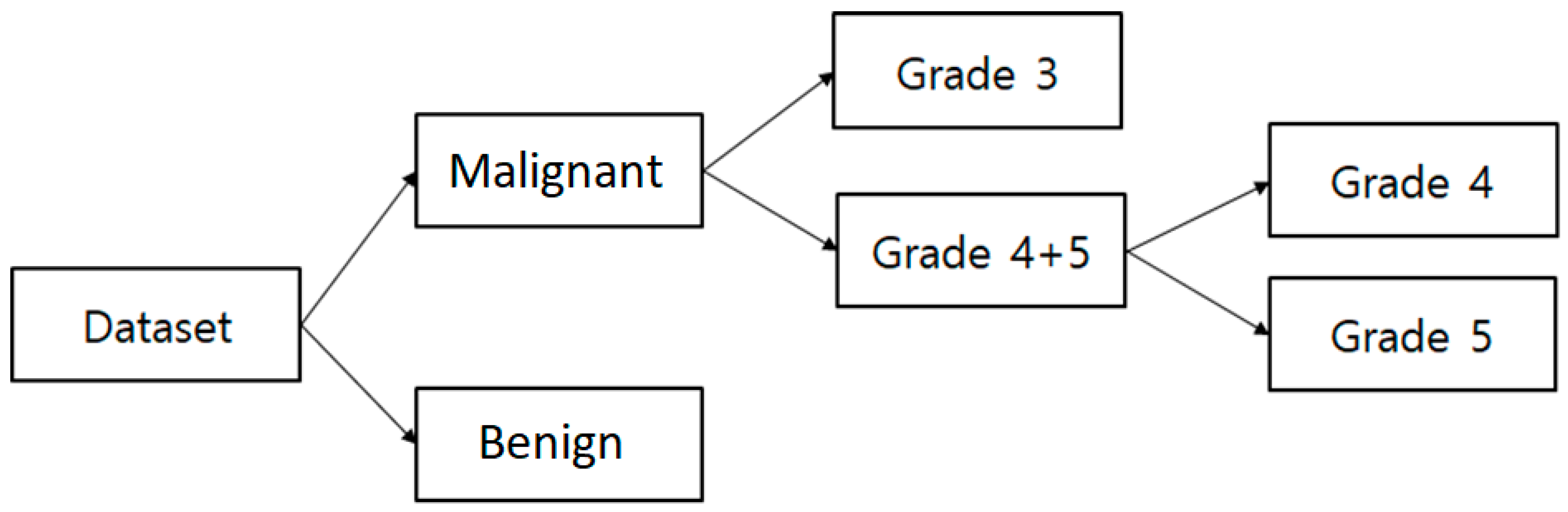
In this paper, 400 images were used in total. Of these, 240 were used for training and 160 were used for testing. The number of images considered for each group was 100, and these were classified as malignant vs. benign, Grade 3 vs. Grade 4+5, and Grade 4 vs. Grade 5. Each image was 24-bits/pixel with a size of 512 × 512 pixels. All of the possible results are shown in Table 2, Table 3 and Table 4, where we show the confusion matrices of SVM binary classification for training and testing separately.
Table 2, Table 3 and Table 4 show the confusion matrices used to evaluate the performance of machine learning algorithms and the classifiers on a set of train and test data. We have shown these confusion matrix tables to get a better idea about the errors of a classification model. Each one of these tables is divided into two parts to show the correctly classified and misclassified data with respect to the training and testing process respectively.
In Table 5, we used four types of performance metrics, namely, accuracy, sensitivity, specificity, and Matthews’s correlation coefficient (MCC). These metrics were calculated using our confusion matrices, i.e., true positive (TP), true negative (TN), false positive (FP), and false negative (FN). We multiplied the accuracy by 100% to normalize it with respect to the other measurements. The four types of performance metrics used in Table 5 are explained as follow,
  • Accuracy is measure of the proportion of correctly classified samples.
    A c c u r a c y = T P + T N T P + T N + F P + F N × 100
  • Sensitivity is a measure of the proportion of positive correctly classified samples.
    S e n s i t i v i t y = T P T P + F N × 100
  • Specificity is a measure of the proportion of negative correctly classified samples.
    S p e c i f i c i t y = T N T N + F P × 100
  • Matthew’s correlation coefficient (MCC) is the eminence of binary class classification. It is a correlation coefficient between target and predictions.
    M C C = T P × T N F P × F N ( ( T P + F N ) ( T P + F P ) ( T N + F N ) ( T N + F P ) ) × 100
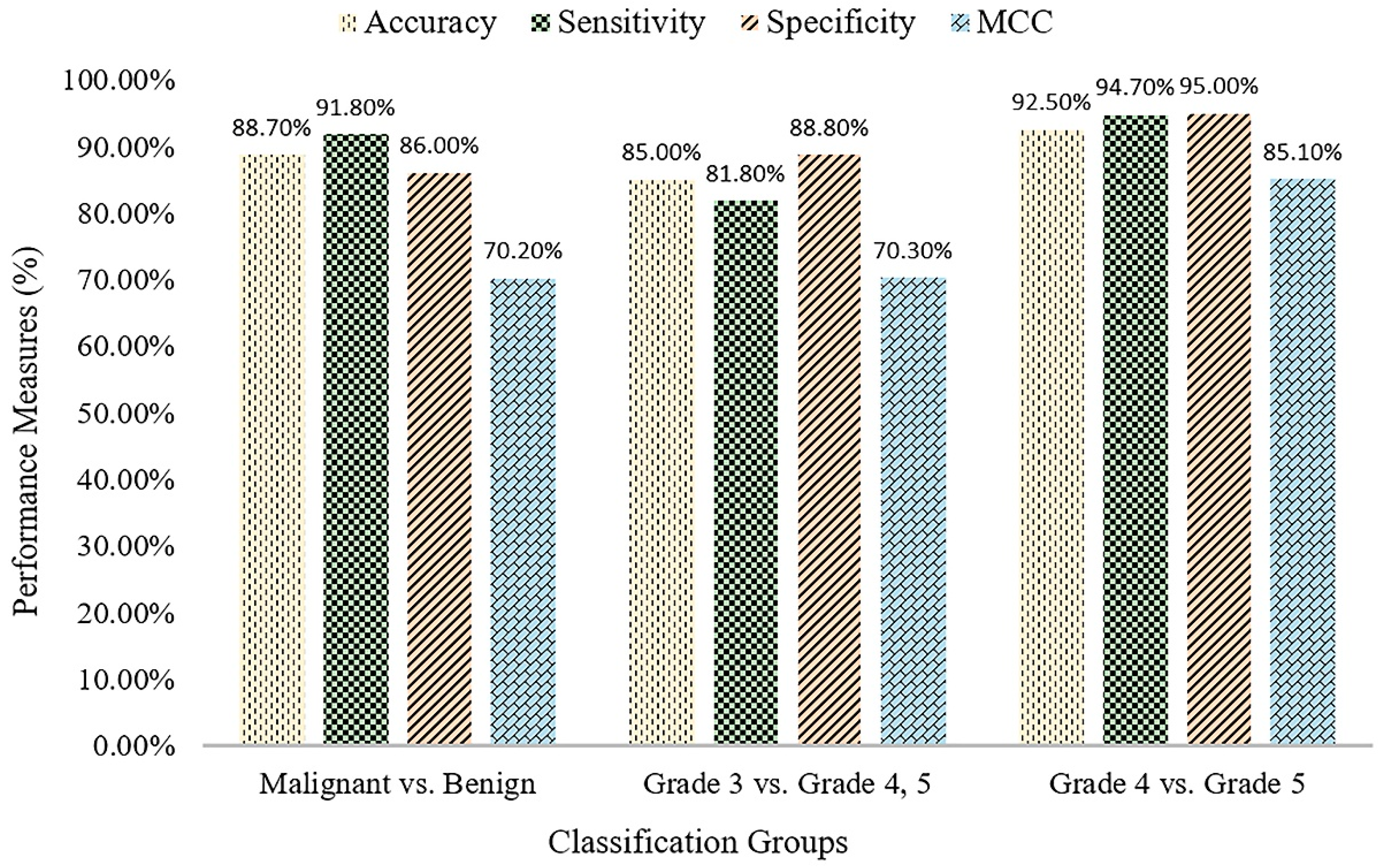
Table 5 shows the classification results of the proposed method for three different groups. The SVM binary classification accuracy, sensitivity, specificity, and MCC for malignant vs. benign are 88.7%, 91.8%, 86.0%, and 70.2%, respectively. For Grade 3 vs. Grade 4+5, the classification accuracy, sensitivity, specificity, and MCC are 85.0%, 81.8%, 88.8%, and 70.3, respectively. For Grade 4 vs. Grade 5, the classification accuracy, sensitivity, specificity, and MCC are 92.5%, 94.7%, 95.0%, and 85.1, respectively.
For the purpose of validation, we also performed prostate cancer grading classification using multilayer perceptron (MLP) technique in Weka, shown in Table 6. MLP is a class of feed-forward artificial neural network, which consists of at least three layers of node: an input layer, hidden layer, and an output layer. Each node is a neuron except input nodes and uses a non-linear activation function. MLP utilizes a supervised learning technique like SVM. From the results shown in Table 5 and Table 6, we can see that the proposed SVM binary classification works significantly better than MLP, and the highest accuracy obtained was 92.5%, for Grade 4 vs. Grade 5. First, classification was performed to detect cancer in all of the samples in the dataset. The second and third classification was performed within the cancer group for low- and high-grade cancer detection. In Figure 7, the bar graph shows the comparison results for the three different binary divisions that are used for SVM classification.
To predict, automatically, prostate cancer gradings, we used machine learning and deep learning algorithms such as SVM and MLP, respectively. To do so, we first applied image segmentation as a preprocessing step. Secondly, we converted the images from RGB to binary to carry out watershed segmentation. Thirdly, we calculated a set of morphological features based on the segmented nucleus and lumen tissue images. Finally, the SVM and MLP classification was performed based on the significant features selected.
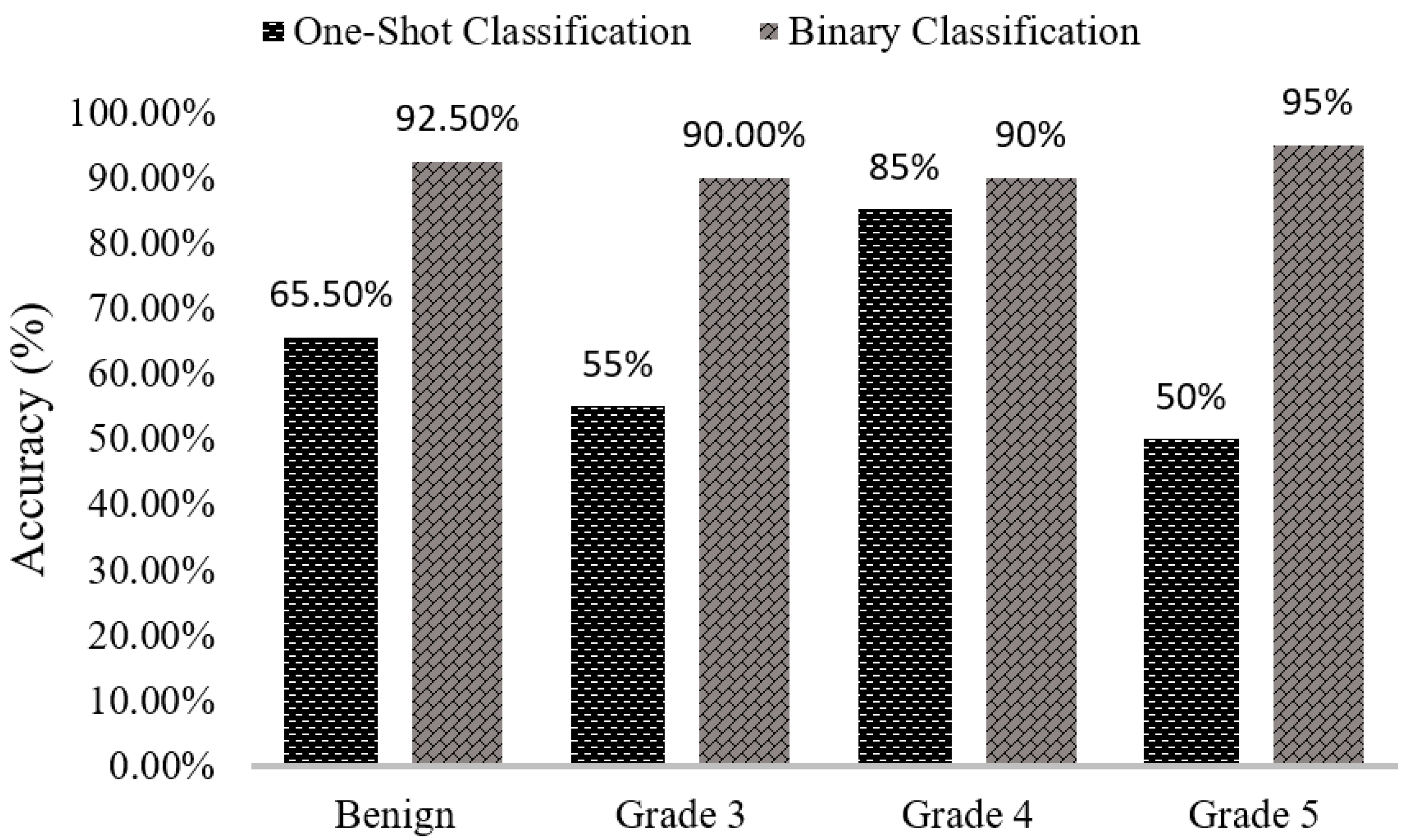
We can see that the results of the comparison between SVM classification accuracy in Table 7 and Figure 8 vary between one-shot and binary classifiers. When we classified our data using multi-class or one-shot classifiers, the classification accuracies for benign, Grade 3, Grade 4, and Grade 5 are 60%, 55%, 85%, and 50%, respectively. Using the proposed binary classification approach, the accuracies for the same groups are 92.5%, 90.0%, 90.0%, and 95.0%, respectively. Comparing both classifiers simultaneously, we can see that the results obtained using the binary classifier are better than those obtained using multi-class or one-shot classifier. Table 8 shows the comparison results of MLP classifier between one-shot and binary classification. After comparing the results between SVM and MLP classification methods, we can say that the proposed method, SVM, achieved better results than MLP. In one-shot classification, the entire dataset is classified into four groups simultaneously. In this case, the errors in one class affect the performance of the others, negatively impacting the classification accuracy. Thus, the model cannot make correct predictions. Whereas, in binary classification, the entire dataset is separated into three groups and each group is classified separately and independently. In this case, the errors in one class do not affect the performance of the other class.
In Table 9, we compare the accuracy of different standard classification methods with our proposed method. The classification accuracy achieved for the class low vs. high grade using the proposed method is higher than other methods described in the literature. On cancer diagnosis, when classified Malignant vs. Benign, our result is better than Nir et al. (2018) and Doyle et al. (2006), but not higher compared to Tabesh et al. (2017), because they used different types of features that are extracted from the tissue image, namely color channel histogram, fractal dimension, fractal code, wavelet, and MAGIC. The authors of Reference [4] computed the features of epithelial nuclei objects in the tissue image, whereas, our method computed the features of all nuclei objects existing in the biopsy prostate tissue image.

5. Conclusions

In this study, we have developed a computerized grading system for digitized histopathology images using supervised learning methods. The segmentation process for biopsy tissue image was performed using the k-means algorithm and touching cells were separated using the watershed algorithm. Morphological features were selected for prostate cancer grading and diagnosis. Gaussian and linear kernels were used for the classification of prostate histopathological images. Using these kernels, we observed some improvements in the results, and gradually increased the performance of the model used for training and testing. The parameters of the kernel play a vital role in the classification process, and the best combination of C and γ was selected for better classification accuracy. Satisfactory classification results were obtained using the extracted morphological features, and these features were extracted from the sub-images, viewable in 40× magnification. The quantitative analysis described here is remarkably flexible in terms of implementation. The SVM binary classification method presented in this paper is used to classify malignant vs. benign, Grade 3 vs. Grade 4+5, and Grade 4 vs. Grade 5. Our results are satisfactory and comparable with those reported in the literature and produced quantitative measures based on the features extracted from microscopic biopsy tissue images. In order to justify our proposed method, SVM, we also carried out features classification using MLP. One-shot and binary classification results were compared to show the differences in two classifications accuracies. In future studies, we will improve our classification accuracy using the combinations of multiple features. Deep learning and machine learning techniques will be used for comparative analysis, where, image classification will be performed using the convolutional neural network (CNN) and feature classification will be performed using support vector machine (SVM), respectively.

Author Contributions

Conceptualization, S.B., H.-G.P. and N.M.; Formal analysis, S.B., D.P., J.-H.S. and N.-H.C.; Methodology, S.B.; Project administration, C.-H.K.; Resources, H.-G.P., C.-H.K. and N.-H.C.; Supervision, H.-K.C.; Validation, S.B.; Visualization, N.M., J.-H.S., N.-H.C. and H.-K.C.; Writing—original draft, S.B.; Writing—review & editing, N.M.

Funding

This research was funded by the Ministry of Trade, Industry, and Energy (MOTIE), Korea, grant number (R&D, P0002072).

Acknowledgments

This research was financially supported by the Ministry of Trade, Industry, and Energy (MOTIE), Korea, under the “Regional Specialized Industry Development Program (R&D, P0002072)” supervised by the Korea Institute for Advancement of Technology (KIAT).

Ethical Approval

All subjects provided written informed consent for their participation in the study, which was approved by the Institutional Ethics Committee at College of Medicine, Yonsei University, Korea (IRB no. 1-2018-0044).

Conflicts of Interest

The authors declare that they have no conflicts of interest.

References

  1. Braunhut, B.L.; Punnen, S.; Kryvenko, O.N. Updates on Grading and Staging of Prostate Cancer. Surg. Pathol. Clin. 2018, 11, 759–774. [Google Scholar] [CrossRef] [PubMed]
  2. Chung, M.S.; Shim, M.; Cho, J.S.; Bang, W.; Kim, S.I.; Cho, S.Y.; Rha, K.H.; Hong, S.J.; Koo, K.C.; Lee, K.S.; et al. Pathological Characteristics of Prostate Cancer in Men Aged < 50 Years Treated with Radical Prostatectomy: A Multi-Centre Study in Korea. J. Korean Med. Sci. 2019, 34, 1–10. [Google Scholar]
  3. Gleason, D.F. Histologic grading of prostate cancer: A perspective. Hum. Pathol. 1992, 23, 273–279. [Google Scholar] [CrossRef]
  4. Tabesh, A.; Teverovskiy, M.; Pang, H.Y.; Kumar, V.P.; Verbel, D.; Kotsianti, A.; Saidi, O. Multifeature Prostate Cancer Diagnosis and Gleason Grading of Histological Images. IEEE Trans. Med. Imaging 2007, 26, 1366–1378. [Google Scholar] [CrossRef] [PubMed]
  5. Doyle, S.; Feldman, M.D.; Shih, N.; Tomaszewski, J.; Madabhushi, A. Cascaded Discrimination of Normal, Abnormal, and Confounder Classes in Histopathology: Gleason Grading of Prostate Cancer. BMC Bioinform. 2012, 13, 282. [Google Scholar] [CrossRef] [PubMed]
  6. Nir, G.; Hor, S.; Karimi, D.; Fazli, L.; Skinnider, B.F.; Tavassoli, P.; Turbin, D.; Villamil, C.F.; Wang, G.; Wilson, R.S.; et al. Automatic grading of prostate cancer in digitized histopathology images: Learning from multiple experts. Med. Image Anal. 2018, 50, 167–180. [Google Scholar] [CrossRef] [PubMed]
  7. Doyle, S.; Madabhushi, A.; Feldman, M.; Tomaszeweski, J. A Boosting Cascade for Automated Detection of Prostate Cancer from Digitized Histology. Comput. Vis.–ECCV 2012 2006, 4191, 504–511. [Google Scholar]
  8. Rundo, L.; Militello, C.; Russo, G.; Garufi, A.; Vitabile, S.; Gilardi, M.C.; Mauri, G. Automated Prostate Gland Segmentation Based on an Unsupervised Fuzzy C-Means Clustering Technique Using Multispectral T1w and T2w MR Imaging. Information 2017, 8, 49. [Google Scholar] [CrossRef]
  9. Jiao, Z.; Gao, X.; Wang, Y.; Li, J. A deep feature based framework for breast masses classification. Neurocomputing 2016, 197, 221–231. [Google Scholar] [CrossRef]
  10. Hu, Y.; Li, J.; Jiao, Z. Mammographic Mass Detection Based on Saliency with Deep Features. Int. Conf. 2016, 292–297. [Google Scholar]
  11. Naik, S.; Doyle, S.; Agner, S.; Madabhushi, A.; Feldman, M.; Tomaszewski, J. Automated gland and nuclei segmentation for grading of prostate and breast cancer histopathology. In Proceedings of the 2008 5th IEEE International Symposium on Biomedical Imaging: From Nano to Macro, Paris, France, 14–17 May 2008; pp. 284–287. [Google Scholar]
  12. Albashish, D.; Sahran, S.; Abdullah, A.; Abd Shukor, N.; Md Pauzi, H.S. Lumen-Nuclei Ensemble Machine Learning System for Diagnosing Prostate Cancer in Histopathology Images. Pertanika. J. Sci. Technol. 2017, 25, 39–48. [Google Scholar]
  13. Nguyen, K.; Sabata, B.; Jain, A.K. Prostate cancer grading: Gland segmentation and structural features. Pattern Recognit. Lett. 2012, 33, 951–961. [Google Scholar] [CrossRef]
  14. Diamond, J.; Anderson, N.H.; Bartels, P.H.; Montironi, R.; Hamilton, P.W. The use of morphological characteristics and texture analysis in the identification of tissue composition in prostatic neoplasia. Hum. Pathol. 2004, 35, 1121–1131. [Google Scholar] [CrossRef] [PubMed]
  15. Ding, Y.; Pardon, M.C.; Agostini, A.; Faas, H.; Duan, J.; Ward, W.O.C.; Easton, F.; Auer, D.; Bai, L. Novel Methods for Microglia Segmentation, Feature Extraction, and Classification. IEEE/ACM Trans. Comput. Boil. Bioinform. 2017, 14, 1366–1377. [Google Scholar] [CrossRef] [PubMed]
  16. Yang, D.; Subramanian, G.; Duan, J.; Gao, S.; Bai, L.; Chandramohanadas, R.; Ai, Y. A Portable Image-Based Cytometer for Rapid Malaria Detection and Quantification. PLoS ONE 2017, 12, 1–18. [Google Scholar] [CrossRef] [PubMed]
  17. Irshad, H.; Veillard, A.; Roux, L.; Racoceanu, D. Methods for Nuclei Detection, Segmentation, and Classification in Digital Histopathology: A Review—Current Status and Future Potential. IEEE Rev. Biomed. Eng. 2014, 7, 97–114. [Google Scholar] [CrossRef] [PubMed]
  18. Majid, M.A.; Huneiti, Z.A.; Balachandran, W.; Balarabe, Y. Matlab as a Teaching and Learning Tool for Mathematics: A Literature Review. Int. J. Arts Sci. 2013, 6, 23–44. [Google Scholar]
  19. Wählby, C.; Lindblad, J.; Vondrus, M.; Bengtsson, E.; Björkesten, L.; Wä Hlby, C.; Bjö Rkesten, L. Algorithms for Cytoplasm Segmentation of Fluorescence Labelled Cells. Anal. Cell. Pathol. 2002, 24, 101–111. [Google Scholar] [CrossRef] [PubMed]
  20. Choi, H.J.; Choi, H.K. Grading of renal cell carcinoma by 3D morphological analysis of cell nuclei. Comput. Boil. Med. 2007, 37, 1334–1341. [Google Scholar] [CrossRef]
  21. Mouelhi, A.; Sayadi, M.; Fnaiech, F.; Mrad, K.; Ben Romdhane, K. Automatic image segmentation of nuclear stained breast tissue sections using color active contour model and an improved watershed method. Biomed. Signal. Process. Control 2013, 8, 421–436. [Google Scholar] [CrossRef]
  22. Shiels, C.; Adams, N.M.; Islam, S.A.; Stephens, D.A.; Freemont, P.S. Quantitative Analysis of Cell Nucleus Organisation. PLoS Comput. Boil. 2007, 3, e138. [Google Scholar] [CrossRef] [PubMed]
  23. Kumar, R.; Srivastava, R.; Srivastava, S. Detection and Classification of Cancer from Microscopic Biopsy Images Using Clinically Significant and Biologically Interpretable Features. J. Med. Eng. 2015, 2015, 1–14. [Google Scholar] [CrossRef] [PubMed]
  24. Choi, H.K.; Jarkrans, T.; Bengtsson, E.; Vasko, J.; Wester, K.; Malmström, P.U.; Busch, C. Image Analysis Based Grading of Bladder Carcinoma. Comparison of Object, Texture and Graph Based Methods and Their Reproducibility. Anal. Cell. Pathol. 1997, 15, 1–18. [Google Scholar] [CrossRef] [PubMed] [Green Version]
  25. Peng, Y.; Jiang, Y.; Yang, C.; Brown, J.B.; Antic, T.; Sethi, I.; Schmid-Tannwald, C.; Giger, M.L.; Eggener, S.E.; Oto, A. Quantitative Analysis of Multiparametric Prostate MR Images: Differentiation between Prostate Cancer and Normal Tissue and Correlation with Gleason Score—A Computer-aided Diagnosis Development Study. Radiology 2013, 267, 787–796. [Google Scholar] [CrossRef] [PubMed]
  26. Doyle, S.; Hwang, M.; Shah, K.; Madabhushi, A.; Feldman, M.; Tomaszeweski, J. Automated Grading Of Prostate Cancer Using Architectural And Textural Image Features. In Proceedings of the 2007 4th IEEE International Symposium on Biomedical Imaging: From Nano to Macro, Arlington, VA, USA, 12–15 April 2007; pp. 1284–1287. [Google Scholar]
  27. Loukas, C.; Kostopoulos, S.; Tanoglidi, A.; Glotsos, D.; Sfikas, C.; Cavouras, D. Breast Cancer Characterization Based on Image Classification of Tissue Sections Visualized under Low Magnification. Comput. Math. Methods Med. 2013, 2013, 1–7. [Google Scholar] [CrossRef]
  28. Emiliozzi, P.; Maymone, S.; Paterno, A.; Scarpone, P.; Amini, M.; Proietti, G.; Cordahi, M.; Pansadoro, V. Increased Accuracy of Biopsy Gleason Score Obtained By Extended Needle Biopsy. J. Urol. 2004, 172, 2224–2226. [Google Scholar] [CrossRef] [PubMed]
  29. Wei, L.; Yang, Y.; Nishikawa, R.M. Microcalcification classification assisted by content-based image retrieval for breast cancer diagnosis. Pattern Recognit. 2009, 42, 1126–1132. [Google Scholar] [CrossRef]
  30. Mazo, C.; Alegre, E.; Trujillo, M. Classification of cardiovascular tissues using LBP based descriptors and a cascade SVM. Comput. Methods Programs Biomed. 2017, 147, 1–10. [Google Scholar] [CrossRef]
  31. Ribeiro, M.G.; Neves, L.A.; Nascimento, M.Z.D.; Roberto, G.F.; Martins, A.S.; Tosta, T.A.A. Classification of colorectal cancer based on the association of multidimensional and multiresolution features. Expert Syst. Appl. 2019, 120, 262–278. [Google Scholar] [CrossRef]
  32. Huang, P.W.; Lee, C.H. Automatic Classification for Pathological Prostate Images Based on Fractal Analysis. IEEE Trans. Med. Imaging 2009, 28, 1037–1050. [Google Scholar] [CrossRef] [Green Version]
  33. Sahran, S.; Albashish, D.; Abdullah, A.; Shukor, N.A.; Pauzi, S.H.M. Absolute cosine-based SVM-RFE feature selection method for prostate histopathological grading. Artif. Intell. Med. 2018, 87, 78–90. [Google Scholar] [CrossRef] [PubMed]
  34. Molina, J.F.G.; Zheng, L.; Sertdemir, M.; Dinter, D.J.; Schönberg, S.; Rädle, M. Incremental Learning with SVM for Multimodal Classification of Prostatic Adenocarcinoma. PLoS ONE 2014, 9, e93600. [Google Scholar]
  35. Cortes, C.; Vapnik, V. Support-Vector Networks. Mach. Learn. 1995, 20, 273–297. [Google Scholar] [CrossRef]
  36. Fondon, I.; Sarmiento, A.; García, A.I.; Silvestre, M.; Eloy, C.; Polónia, A.; Aguiar, P. Automatic classification of tissue malignancy for breast carcinoma diagnosis. Comput. Boil. Med. 2018, 96, 41–51. [Google Scholar] [CrossRef] [PubMed]
  37. Liang, C.; Bian, Z.; Lv, W.; Chen, S.; Zeng, D.; Ma, J. A computer-aided diagnosis scheme of breast lesion classification using GLGLM and shape features: Combined-view and multi-classifiers. Phys. Medica. 2018, 55, 61–72. [Google Scholar] [CrossRef] [PubMed]
  38. Li, J.; Weng, Z.; Xu, H.; Zhang, Z.; Miao, H.; Chen, W.; Liu, Z.; Zhang, X.; Wang, M.; Xu, X.; et al. Support Vector Machines (SVM) classification of prostate cancer Gleason score in central gland using multiparametric magnetic resonance images: A cross-validated study. Eur. J. Radiol. 2018, 98, 61–67. [Google Scholar] [CrossRef] [PubMed]
  39. Hai, J.; Tan, H.; Chen, J.; Wu, M.; Qiao, K.; Xu, J.; Zeng, L.; Gao, F.; Shi, D.; Yan, B. Multi-level features combined end-to-end learning for automated pathological grading of breast cancer on digital mammograms. Comput. Med. Imaging Graph. 2019, 71, 58–66. [Google Scholar] [CrossRef] [PubMed]
  40. Doyle, S.; Feldman, M.; Tomaszewski, J.; Madabhushi, A. A Boosted Bayesian Multiresolution Classifier for Prostate Cancer Detection from Digitized Needle Biopsies. IEEE Trans. Biomed. Eng. 2012, 59, 1205–1218. [Google Scholar] [CrossRef]
Figure 1. Microscopic biopsy images stained with Hematoxylin and Eosin (H&E) compound; (ad) whole slide tissue images of Grade 3, Grade 4, Grade 5, and Benign; and (eh) the regions of interest (ROIs) taken from whole-slide images (a), (b), (c), (d) respectively. The dark blue is the cell nucleus, pink is the stroma, and white is the lumen.
Applsci 09 02969 g001
Figure 2. Proposed pipeline model for predicting cancer grading from microscopic biopsy images.
Applsci 09 02969 g002
Figure 3. Image segmentation using K-means algorithm: (a) original tissue image; (b) lumen segmentation; and (c) nucleus segmentation.
Applsci 09 02969 g003
Figure 4. Overview of watershed segmentation: (a) original segmented image of nucleus tissue components; (b) noise-removed binary image; (c) Euclidean distance transform on binary image; and (d) result of the watershed algorithm and labelled nuclei using color mapping.
Applsci 09 02969 g004
Figure 5. Improvement of over-segmentation: (a) over-segmented objects; (b) markers applied to the inverse results of the distance transform; (c) applied watershed algorithm on images (b); and (d) the resulting image after removing the noise and watershed line, and the centroid of the nucleus has been labelled.
Applsci 09 02969 g005
Figure 6. Proposed binary method for support vector machine (SVM) classification. Three different classifiers have been used here for binary classification and each group is classified independently and separately.
Applsci 09 02969 g006
Figure 7. Comparison graph of support vector machine (SVM) classification accuracy among three binary divisions. The classification accuracies of the three groups are very close to each other, and the highest accuracy obtained was 92.50%, for grade 4 vs. grade 5. Matthew’s correlation coefficient (MCC) indicates the quality of binary classification among the three classification groups.
Applsci 09 02969 g007
Figure 8. Comparison between support vector machine (SVM) classifiers among the four Gleason grade groups. In the case of one-shot classification, the classifier could not accurately distinguish among the four groups. In the case of binary classification, the classifier was almost always accurate, with little variation.
Applsci 09 02969 g008
Table 1. Proposed features for support vector machine (SVM) binary classification to classify Gleason grading of prostate cancer.
Feature TypeFeature Description
Nucleus featuresArea, perimeter, major axis length, minor axis length, circularity, diameter, compactness, nucleus to nucleus average distance, nucleus to nucleus minimum distance
Lumen featuresArea, perimeter, major axis length, minor axis length, eccentricity
Table 2. Confusion matrix of SVM binary classification—Malignant vs. Benign.
Training: 99.2%Testing: 88.7%
TrainMalignantBenignDataTestMalignantBenignData
Malignant60060Malignant34640
Benign15960Benign33740
Table 3. Confusion matrix of SVM binary classification—Grade 3 vs. Grade 4, 5.
Training: 91.7%Testing: 85.0%
TrainGrade 3Grade 4+5DataTestGrade 3Grade 4+5Data
Grade 355560Grade 336440
Grade 4+555560Grade 4+583240
Table 4. Confusion matrix of SVM binary classification—Grade 4 vs. Grade 5.
Training: 95.0%Testing: 92.5%
TrainGrade 4Grade 5DataTestGrade 4Grade 5Data
Grade 454660Grade 436440
Grade 506060Grade 523840
Table 5. Evaluation results and performance metrics for three binary divisions using SVM.
GroupsAccuracy (%)Sensitivity (%)Specificity (%)MCC (%)
Malignant vs. Benign88.791.886.070.2
Grade 3 vs. Grade 4, 585.081.888.870.3
Grade 4 vs. Grade 592.594.795.085.1
Table 6. Evaluation results for three binary divisions using the multilayer perceptron (MLP) classification technique.
GroupsTraining Accuracy (%)Testing Accuracy (%)
Malignant vs. Benign99.081.0
Grade 3 vs. Grade 4, 598.075%
Grade 4 vs. Grade 597.576.25
Table 7. Support vector machine (SVM) classifier, comparison between one-shot and binary classification.
One-Shot ClassificationBinary Classification
GroupsAccuracy (%)GroupsAccuracy (%)
Benign60.0Benign92.5
Grade 355.0Grade 390.0
Grade 485.0Grade 490.0
Grade 550.0Grade 595.0
Total65.5Total92.0
Table 8. Multilayer perception (MLP) classifier, comparison between one-shot and binary classification.
One-Shot ClassificationBinary Classification
GroupsAccuracy (%)GroupsAccuracy (%)
Benign37.5Benign87.5
Grade 367.5Grade 390.0
Grade 445.0Grade 475.0
Grade 570.0Grade 577.5
Total55.5Total82.5
Table 9. Comparison between the proposed method and other standard methods for the classification of prostate cancer gradings.
AuthorsClassification MethodsClassesAccuracy
Tabesh et al. (2007) [4]kNNMalignant vs. Benign96.7%
Low vs. High Grade81.0%
Doyle et al. (2012) [5]Decision Tree (DT)Grade 377.0%
Grade 476.0%
Grade 595.0%
Nir et al. (2018) [6]SVMMalignant vs. Benign88.5%
Low vs. High Grade73.8%
Doyle et al. (2006) [7]BayesianMalignant vs. Benign88.0%
Rundo et al. [8]Fuzzy C-MeansMultispectral (Tw1 & Tw2)90.77%
Naik et al. [11]SVMGrade 3 vs. Grade 495.19%
Benign vs. Grade 386.35%
Benign vs. Grade 492.90%
Albashish et al. (2017) [12]SVMGrade 3 vs. Grade 488.9%
Benign vs. Grade 397.9%
Benign vs. Grade 492.4%
Nguyen et al. (2012) [13]SVMBenign, Grade 3, and
Grade 4 carcinoma
85.6%
ProposedSVMMalignant vs. Benign88.7%
Low vs. High Grade85.0%
Grade 4 vs. Grade 592.5%
Grade 390.0%
Grade 490.0%
Grade 595.0%

