Article

Algorithm Development for the Non-Destructive Testing of Structural Damage

by
Azadeh Noori Hoshyar
1,*,
Maria Rashidi
1,
Ranjith Liyanapathirana
2 and
Bijan Samali
1
1
Centre for Infrastructure Engineering (CIE), Western Sydney University, Kingswood, NSW 2747, Australia
2
School of Computing, Engineering and Mathematics, Western Sydney University, Kingswood, NSW 2747, Australia
*
Author to whom correspondence should be addressed.
Appl. Sci. 2019, 9(14), 2810; https://doi.org/10.3390/app9142810
Submission received: 21 May 2019 / Revised: 24 June 2019 / Accepted: 1 July 2019 / Published: 13 July 2019
(This article belongs to the Section Civil Engineering)

Abstract

:
Monitoring of structures to identify types of damages that occur under loading is essential in practical applications of civil infrastructure. In this paper, we detect and visualize damage based on several non-destructive testing (NDT) methods. A machine learning (ML) approach based on the Support Vector Machine (SVM) method is developed to prevent misdirection of the event interpretation of what is happening in the material. The objective is to identify cracks in the early stages, to reduce the risk of failure in structures. Theoretical and experimental analyses are derived by computing the performance indicators on the smart aggregate (SA)-based sensor data for concrete and reinforced-concrete (RC) beams. Validity assessment of the proposed indices was addressed through a comparative analysis with traditional SVM. The developed ML algorithms are shown to recognize cracks with a higher accuracy than the traditional SVM. Additionally, we propose different algorithms for microwave- or millimeter-wave imaging of steel plates, composite materials, and metal plates, to identify and visualize cracks. The proposed algorithm for steel plates is based on the gradient magnitude in four directions of an image, and is followed by the edge detection technique. Three algorithms were proposed for each of composite materials and metal plates, and are based on 2D fast Fourier transform (FFT) and hybrid fuzzy c-mean techniques, respectively. The proposed algorithms were able to recognize and visualize the cracking incurred in the structure more efficiently than the traditional techniques. The reported results are expected to be beneficial for NDT-based applications, particularly in civil engineering.

1. Introduction

Structural health monitoring (SHM) using non-destructive inspection (NDI) has been known as one of the technologies in which the material properties can be evaluated without the occurrence of any damages A. NDI and Non-destructive Testing (NDT) methods rely on the employment of electromagnetic waves and intrinsic characteristic attributes of materials to test samples. One of the most commonly known NDI/NDT techniques is ultrasonic inspection, which engages transducers to generate mechanical oscillations through the inspected material, and receives the reflected ultrasonic waves from the material [1]. The analysis of this data has the potential to detect structural damage in the early stages, by minimizing errors, and thus reducing the asset management costs. Despite the vast number of studies in this field, few robust methods have been proven to indicate an adverse condition of a structure in service. Also, many researchers have concentrated on the automated detection of defects [2,3,4,5,6,7,8,9,10,11,12], but few studies have been done into the comprehensive or well-ordered data analysis of systems, and hence this is the motivation for the present research.
The solution requires a classifier that can discriminate structures as either being damaged or intact. Concerning AI techniques, the most commonly used classifiers are based on Discriminant Analysis, Artificial Neural Network, K-Nearest Neighborhood, Support Vector Machine (SVM), Support Vector Regression, Adaptive Neuro-Fuzzy System (ANFIS), Fuzzy Inference System (FIS) and Decision Trees. These algorithms have successfully been utilized to solve engineering problems [3,4,5,6,13,14,15]. The SVM method has been extensively used in many research studies, and it is accepted as an efficient classifier for detecting damage [7,8,9]. However, there had been a substantial increase in utilizing advice sets for enhancing SVM performance. However, applying and expressing this knowledge in terms of its constraints still has some difficulties. These techniques require new parameters and operations that can enhance the SVM computational cost. In this regard, the first contribution of this study is to develop non-iterative SVM-based algorithms for analyzing the sensor (smart aggregate) data, which can improve the performance of SVM, rather than traditional SVM.
Furthermore, the local structural health monitoring based on microwave and millimeter-wave imaging is an efficient approach for visualizing and localizing detected damage in structures [10,11,12,16,17,18]. These methods offer cost-effective methods of local inspection, to identify the exact location of the crack [19,20]. Microwave- and millimeter imaging techniques are non-contact and one-sided techniques which can be efficiently applied for the non-destructive evaluation of non-transparent materials, as their signals can penetrate the dielectric materials and provide information about the entire structure [21,22]. In other words, these techniques examine microwave pulses or continuous wave signals, to offer comprehensive descriptions of the systems. In common microwave imaging inspections, the reflection from the test specimen is recorded by the radio frequency (RF) detector, and it is used for the detection of damage inside the specimen [21,23,24]. In general, to obtain the desired range resolution and 3D images, relatively complex wide-frequency range measurement systems and image processing algorithms are required. In many applications, wide band techniques may not be applicable, due to specific requirements, such as the depth of penetration in composite materials, and the cost of the techniques. However, there are various microwave- and millimeter-wave imaging systems that have been used for NDT in structures, including relatively simple single-frequency reflectometers [10,21,22,25], and also relatively complex wide-band reflectometers, such as synthetic aperture radar (SAR) [11,26]. However, most of the generated images have very low resolution, in which the investigating object is not recognizable. Therefore, the proper image processing techniques [27] are required to handle the imaging data. In this regard, the second contribution of this study is to develop algorithms using image processing techniques to create enhancement and segmentation of obtained microwave images of civil structures for the recognition of anomalies, and to obtain the area of interest. In contrast to the results of prior research [22], this study performs a systematic investigation of the problem, and this is followed by various image processing approaches. The methodology of this research relies on modern computer vision techniques, instead of traditional photogrammetric methods.
The remainder of the paper is organized as follows: The damage detection technique based on ML is described in Section 2 of this paper. Then, damage detection and visualization, using the microwave- and millimeter-wave imaging systems are presented in detail. Third, experimental setups are explained, and then the experimental results are investigated, to evaluate the validity of the proposed data analysis procedure, in the Results and Discussion. This is followed by a discussion, and finally conclusions.

2. Damage Detection Using a Machine Learning Approach

2.1. Support Vector Machine

Support vector machine (SVM) is a discriminative classifier which was proposed in 1995 by Vapnik, to analyze data for classification and regression purposes [28]. SVM provides the optimal hyperplane by separating two classes with the maximum margin from the hyperplane. Assume an SVM binary classification with N samples in the data training set ( x 1 , y 1 ) , , ( x i , y i ) , , ( x N , y N ) R n × { ± 1 } , where x i is a feature vector and y i is the label of its class. The hyperplane is mathematically defined as the pair (w, b) in the form: wTx + b = 0, where w is a weight vector and b is the bias. The hyperplane should meet the following condition as described in Equation (1), when linearly separating the training data [29]:
y i ( w × x i + b ) 1 ,     i = 1 , , N
The distance between the hyperplane and each of the training data x i is defined through Equation (2) as [29]:
d i = w × x i + b w
By considering both Equations (1) and (2), the following result is obtained for all x i as [29]:
y i d i 1 w
where 1 w is considered as the lower distance bound between the hyperplane and the training data x i . The maximum margin of the hyperplane is obtained through the minimization of Equation (4):
z = 1 2 w × w
Therefore, the final decision function is given as [30]:
f ( x ) = sign ( α i > 0 y i α i < x , x i > + b )
where ( α 1 ,   α 2 , , α N ) represents the non-negative Lagrange multipliers related to the constraints (see Equation (1)). However, most of these α are usually zero, leading to the small proportion of the training data x being considered as vector w. Since these points are considered as the closest points to the hyperplane, they are named the Support Vectors (SV). SVs are the training patterns that fall on the margin boundaries. In general, a small portion of the training sample SVs are used by SVM for the purpose of classification. However, if the SVs consist of the training data beyond the corresponding margins, they are referred to as misclassified data [31,32,33]. If the linear separation of data is not feasible, then the hyperplane is pointless. Therefore, N non-negative ( ξ i ,   i = 1 , , N ) variables are considered, such that:
y i ( w × x i + b ) 1 ξ i
This variable, ξ i , will include a very small quantity of misclassified points, and this will be zero if the Equation (1) condition is met; otherwise the term ξ will be added to Equation (1), and this generates Equation (6). However, the tolerance parameter may also cause the ignorance of some training data in order to make the linear hyperplane. Then, the generalized separation hyperplane is expressed by minimizing Equation (7):
z = 1 2 w × w + c i = 1 N ξ i
The expression c i = 1 N ξ i will supervise the number of misclassified points. For smaller values of c, the above solution maximizes the minimum distance of 1/w, and for large values of c, it minimizes the number of misclassified data. It is noted that the use of misclassified data can help to enhance the performance of classifiers.

2.2. Developed Support Vector Machine

In the implementation of a traditional SVM algorithm, the first type of support vectors or hyperplane position is the only information that is utilized in the test phase of SVM from the training phase, while the purpose of this algorithm is utilizing the second type of support vectors to provide the subsequent knowledge by the purpose of enhancement in SVM performance. The second type of support vectors is selected, as there is a lot of misclassified data, even in the existence of the optimized hyperplane [31]. Two potential sources of this misclassified data are the outliers and the non-linear separable data when using kernels. Traditional SVM do not consider non-linear separable data during the training phase. This happens in defining the constraints and also the tolerance parameters of the objective functions. The main concern herein is that if the data in the test set appears to be practically the same as these misclassified data in the training set, they will be essentially classified incorrectly as being misclassified data. This misclassification may reduce accuracy, as it happens because the SVM ignores the information in the training phase. Therefore, in order to obtain the benefits from misclassified data, the outlier’s effect should be taken into account. Searching to find more similar data to the misclassified data, as proposed in this research, can enhance SVM performance. In this method, after determining the misclassified data in the training phase, the SVM will provide the advice weights, which are used in conjunction with the decision values in the testing phase. These defined advised weights will help SVM to improve its accuracy, while eliminating the outlier data. Equation (8) expresses the obtained misclassified data of the training phase as [29]:
MD = i = 1 N x i | y i sign ( α j > 0 y j α j k ( x i , x j ) + b )
The right side of the above equation may include any SVM decision function. Although there is the possibility that misclassified data may be null, experimental results have shown that the incidence of the misclassified data is prevalent. For each misclassified data in the MD set, the length from the corresponding k-nearest neighbor (k = 10) that has been correctly classified is computed as:
CL ( x i ) = Minimum x j ( cl ( x i ) cl ( x j ) )
N = 1 , 2 , , 10 ,   y i # y j
cl ( x i ) = x i   M d
cl ( x j ) = x j   M d
M d = 1 N j = 1 N ( x i x j )
where CL ( x i ) is the dispersion of the misclassified data from the 10-nearest neighbors that have been correctly classified. M d represents the average of the distances within the k-nearest neighbor (k = 10) of x i . However, by mapping the training data into a higher dimension, Equation (13) can be used with respect to kernel k to compute the length as:
( θ cl ( x i ) θ cl ( x j ) ) ) = ( k ( cl ( x i ) , cl ( x i ) ) ) + ( k ( cl ( x j ) , cl ( x j ) ) ) 2 k ( cl ( x i ) , cl ( x j ) ) 0.5
where k ( cl ( x n ) , cl ( x n ) ) = ø ( cl ( x n ) ) · ø ( cl ( x n ) )   { n = i   o r   j } , and represents the Kernel function. It defines the inner product in the transformed space, and reduces the complexity of finding the mapping function.
By computing the CL for each xk in the test set, the self-weightings (SWs) are assigned as:
W = { 0    x i   MD   if   MD   is   empty   or   ( | | cl   ( x k ) cl   ( x i ) | | ) >   CL   ( x i ) 1 xi | | cl   ( x k )   cl   ( x i ) | | xi CL   ( x i )   x i M   if   MD   is   empty   or   ( | | cl   ( x k ) cl   ( x i ) | | ) CL   ( x i )
The obtained SWs show the closeness of the test data to the misclassified data in the training phase. Therefore, the developed self-weighting SVM (SW-SVM) can be concluded as follows:
  • In the training phase, perform the SVM training.
  • Use Equation (8) to find the misclassified data (MD).
  • Investigate the existence of misclassified data maintained in a MD structure; if the MD includes the data, the CL is computed through Equation (9) for each member of MD; otherwise the normal SVM procedure is continued.
  • In the testing phase, compute the self-advised weights of each xk in the test set.
  • For each xk in the test set, the absolute values of the SVM decision values are computed, and normalized or scaled to [0,1].
  • The SVM labelling is followed, based on the conditions in Equation (14). The normal SVM labelling is performed if SW (xk) < decision value (xk).

3. Damage Visualization

3.1. Developed Image Processing Algorithms

The proposed algorithms are used to visualize and detect the suspected critical cracks, using a spot measurement on the structures. The basis of this section relies on the fact that the structural components provide pixels that are visible to the high-resolution sensors, which can demonstrate the topographical appearance characteristics of structural integrity. The changes in structural integrity can be recognized by the variation of image intensities at different intervals. To begin with, upon the antenna measurements of the specimens, the information of the returned signals from the target was gathered as the raw data. The recorded data included the magnitude and phase at different frequencies. This data was processed to achieve a two-dimensional image, through Fourier Transform (FT). The phase and magnitude at each frequency were multiplied by a ‘Kaiser’ window function to minimize the FFT affect over non-integer numbers. The windowed frequency data was transformed to the time-domain, by employing an inverse Fourier transform. Therefore, the antenna time-domain measurement result was subsampled as an image in Matlab.

3.1.1. Pre-Processing

The obtained images were converted into greyscale, in which the minimum intensity value was equal to 0, and the maximum intensity value was equal to 255 [34]. Then, the averaging filter and contrast enhancement techniques were used to precede the enhancement of the raw images. Enhancement in this case, consists of smoothing the image while preserving as much of its grey tonality as possible. Moreover, computational efficiency is an essential consideration in image processing, due to the size of data sets. Some filters, such as average filter, can be implemented by division into two simpler filters, lead to substantial time savings [27]. Assume an n × n filter that can be separated into two smaller sizes of n × 1 and 1 × n. The performance of the n × n filter involves n2 multiplications, and also n2 − 1 additions for every pixel in an image, while the performance of n × 1 filter only requires n multiplications and n−1 additions. In total, the two smaller filters involve 2n multiplications and 2n − 2 additions. This efficiency savings is dramatic when n is large [27,35]. Therefore, in this study, a rectangular averaging filter size of 3 × 3 was considered and implemented by division into two smaller filters. Firstly, 3 × 1 average filters were applied to the raw image, and then a 3 × 1 average filter preceded the result. The new grey values of the corresponding pixel were calculated by taking the average of all nine values in the 3 × 1 and 3 × 1 masks. This process was followed by a Gamma transformations function to adjust the intensity. With Gamma transformations, the grayscale components can be curved to either brighten or darken the intensity [36]. The MATLAB function, imadjust (), was used herein to create Gamma transformations. Since our images were of the class ‘uint8′, the function multiplied the values by 255 to specify the actual values of an image. After pre-processing of images, cluster analysis was carried out for steel plate (SP), composite materials (CM), and metal plate (MP) images.

3.1.2. Cluster Analysis

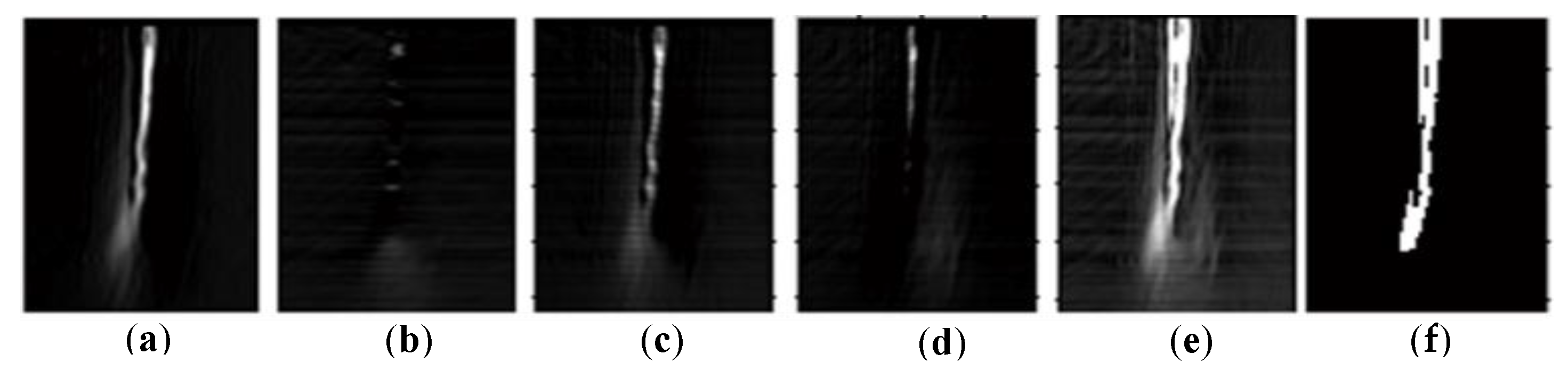
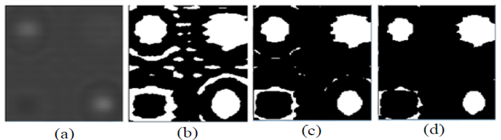
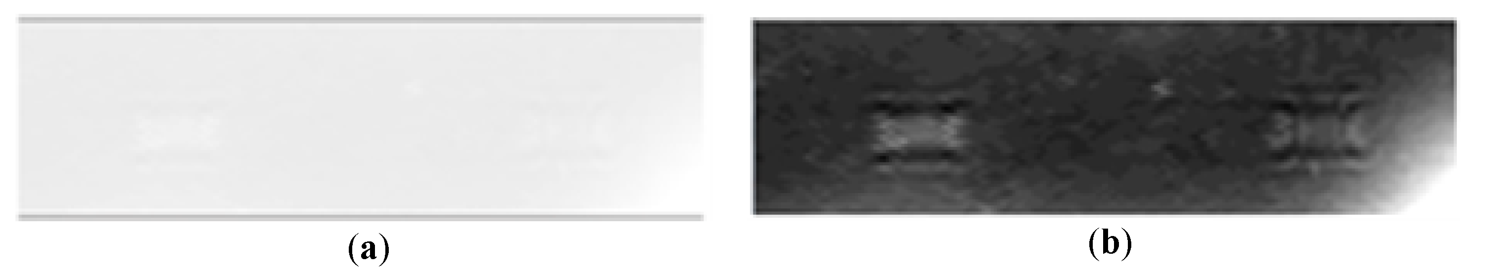
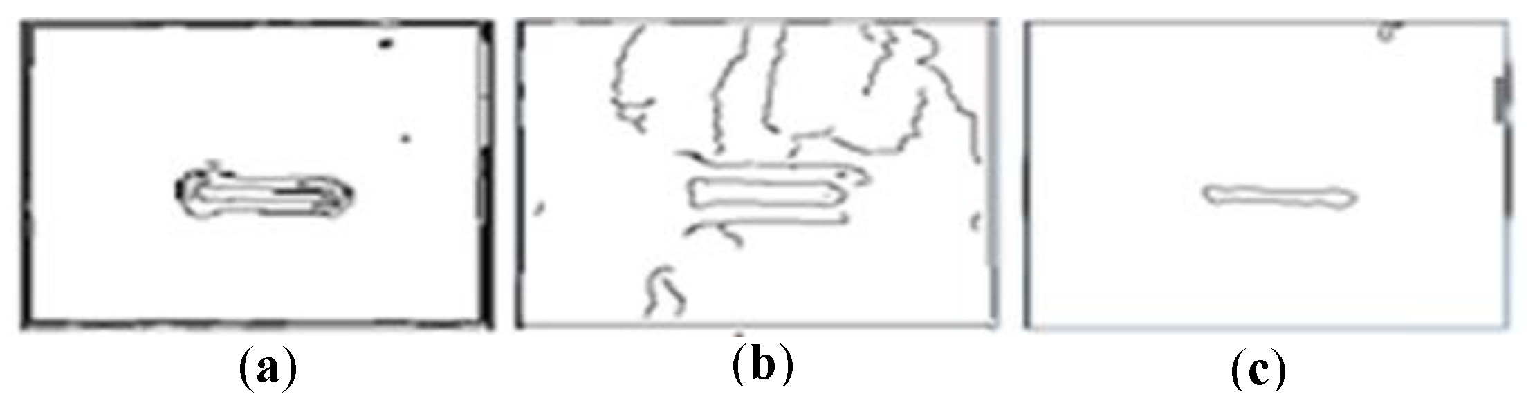
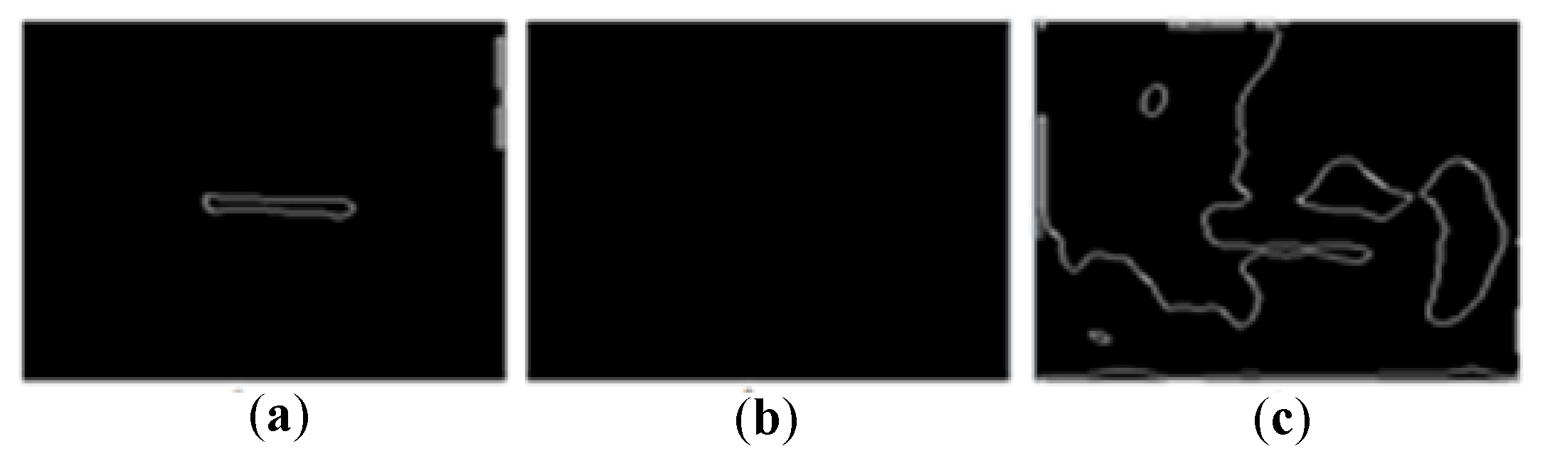
3.1.2.1. Segmentation of Steel Plate (SSP) Images

The gradient magnitude was calculated on pre-processed SP images by computing the gradients in four directions of an image with the Prewitt filter. The edges of the crack were returned at those points where the gradient of the image was maximized. Therefore, the edges were obtained by using the Prewitt approximation to the derivative. Assuming the profile of the image as f(x), the detailed pseudocode of this algorithm is described as follows.
Pseudocode 1. The proposed FT-based algorithms for defect segmentation in microwave imaging.
Input: Phase and Magnitude
Output: True Target Segmentation
1. Pre-processing of SP images as in Section 1.
2. Computation of the derivative of the input microwave image as f′(x) to identify the direction of the maximum changes:
dy dx = lim h 0 ( f ( x + h ) f ( x h ) h )
where h has the value of ‘1’ as the smallest possible value that can occur in an image; therefore, the discrete version of the derivative expression is the form of:
f ( x + 1 ) f ( x 1 )
3. Consideration of the horizontal, vertical, and diagonal filters based on Prewitt approximation in four directions: These filters find horizontal, vertical, and diagonal edges in an image while smoothing the results.
P x = ( 1 0   1 1 0 1 1 0 1 )    Vertical   filter
P y = P x      Horizontal   filter
P d 1 = ( 0   1 1 1 0 1 1 1 0 )    Diagonal   filter   ( Right   to   left )
P d 2 = ( 1 1 0 1 0 1 0 1 1 )    Diagonal   filter   ( Right   to   left )
4. Assuming that Px, Py, Pd1, and Pd2 as the grey values produced by applying the above filters to an image, the gradient magnitude is computed by:
GM = p x 2 + p y 2 + p d 1 2 + p d 2 2
5. Computing the threshold value of the image by Otsu’s thresholding method.
6. Generating the binary image that contains edges by only applying the threshold value.

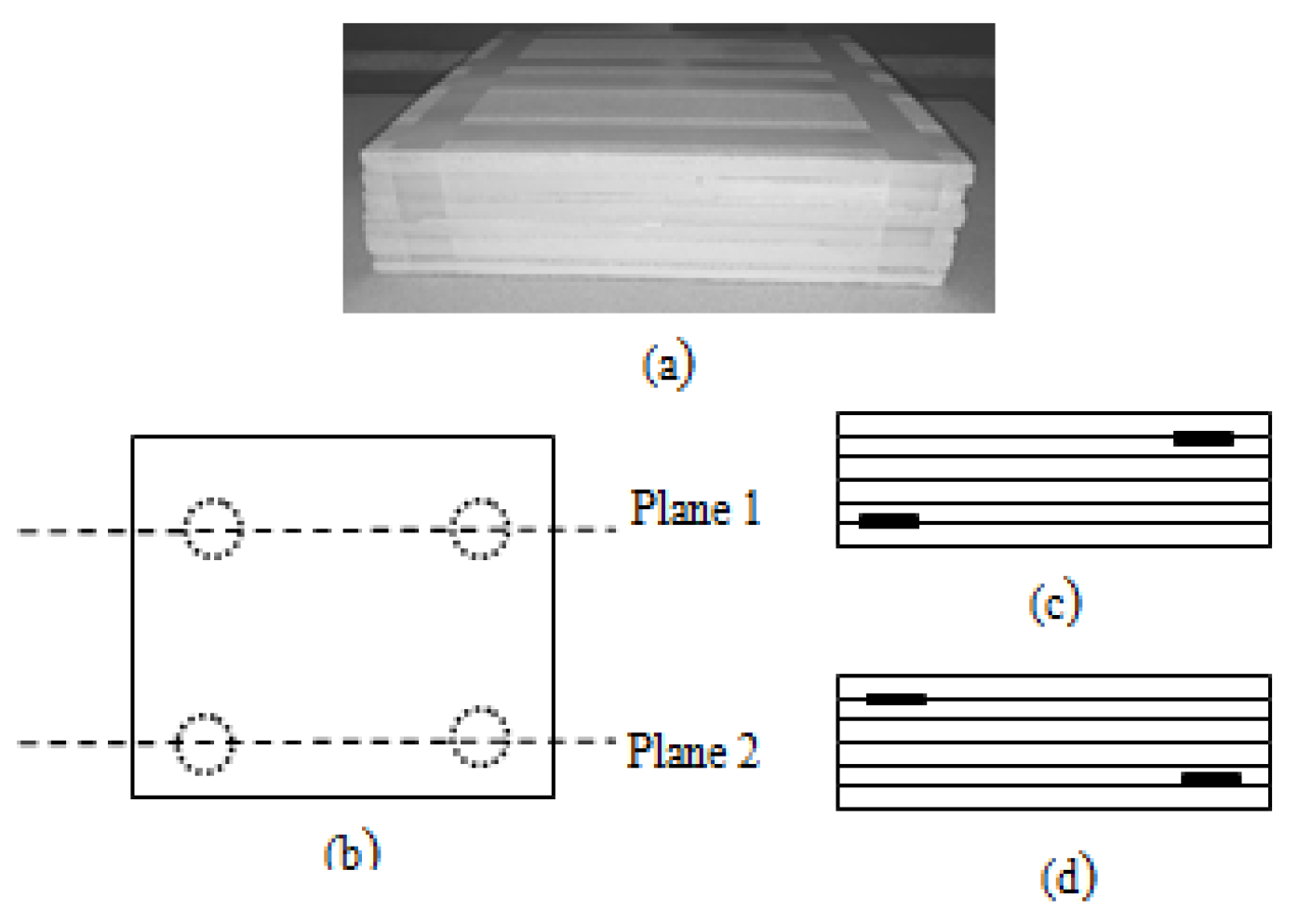
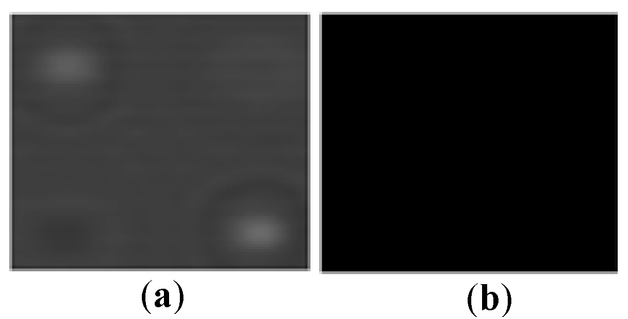
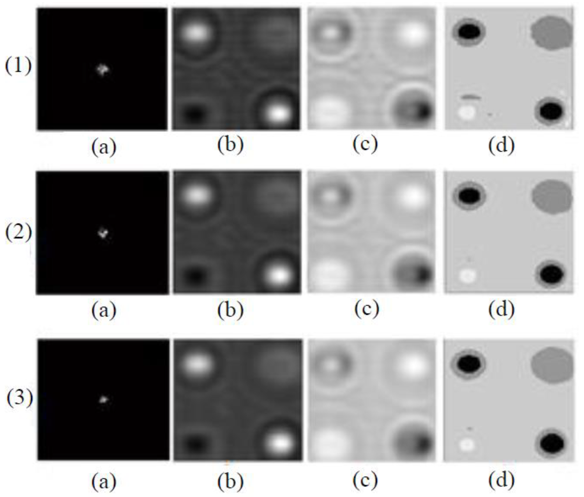
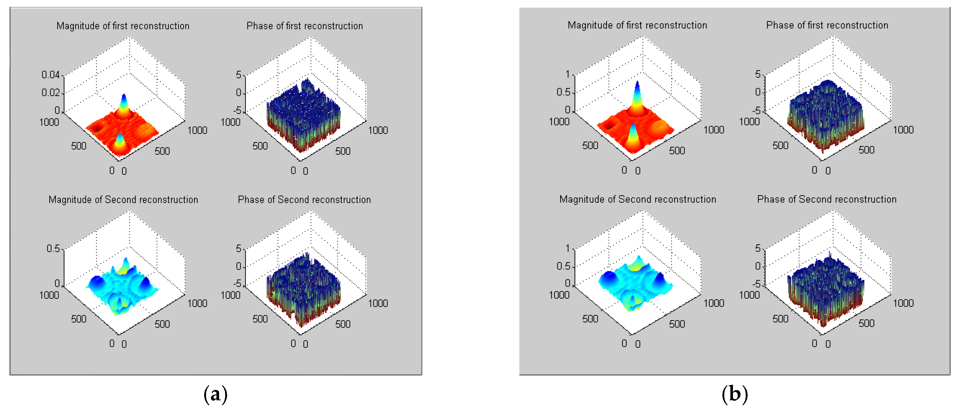
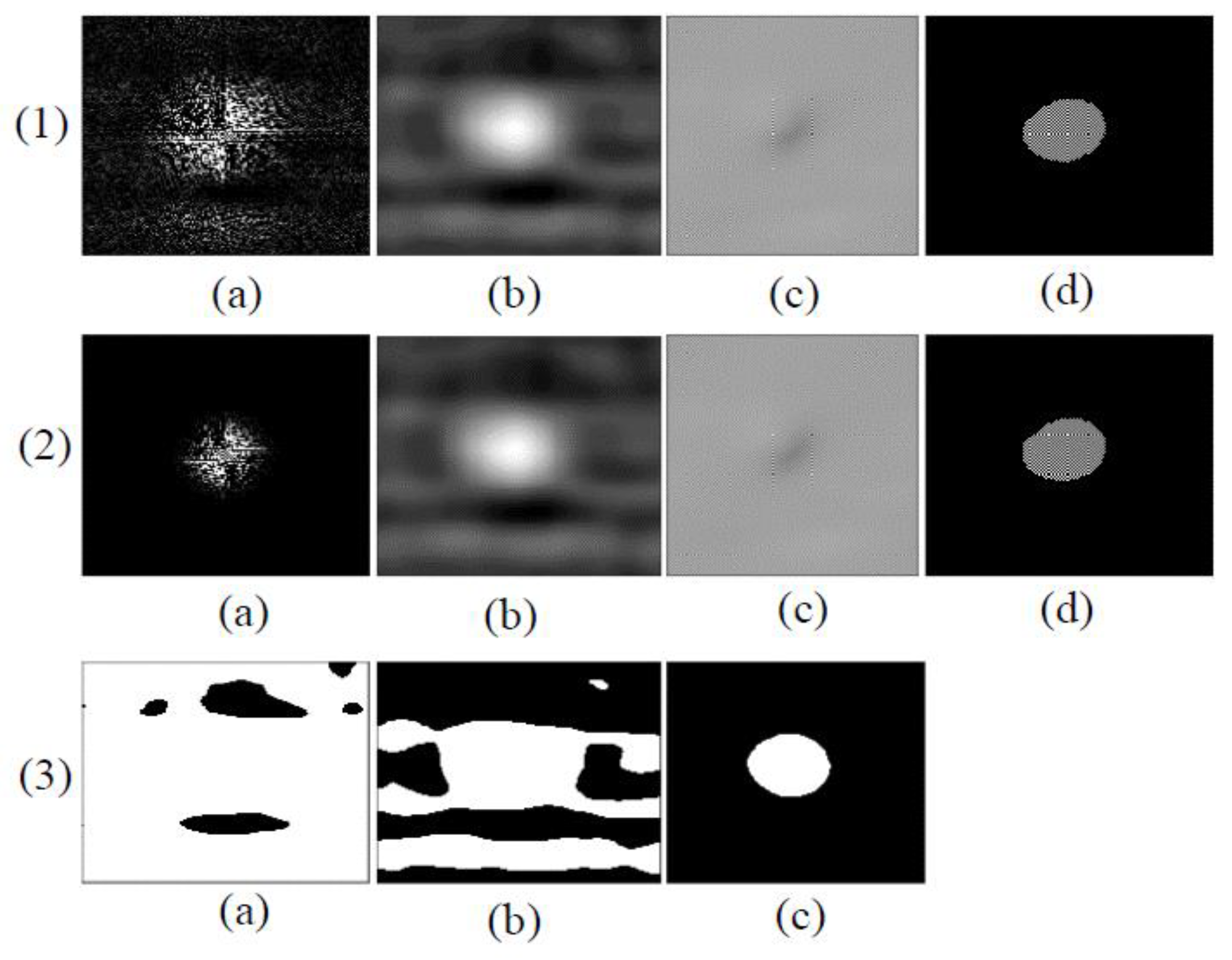
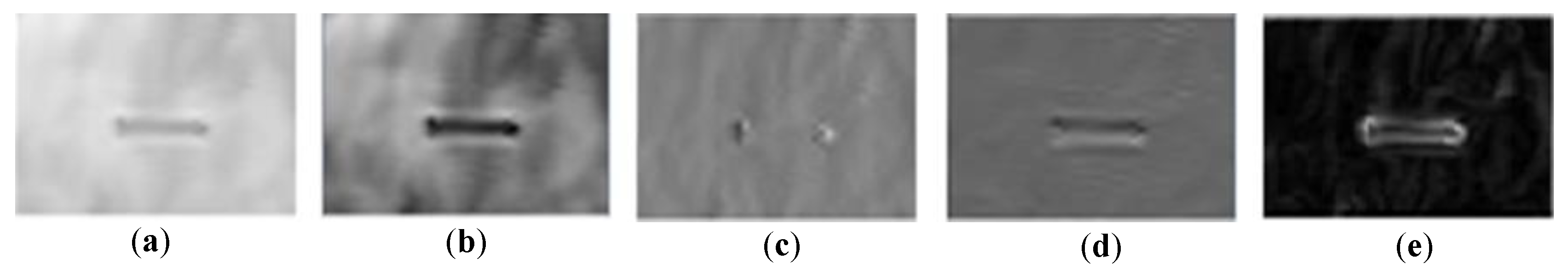
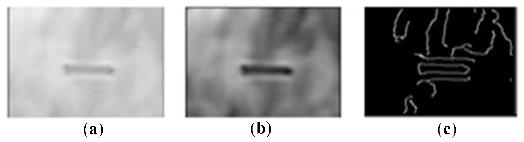
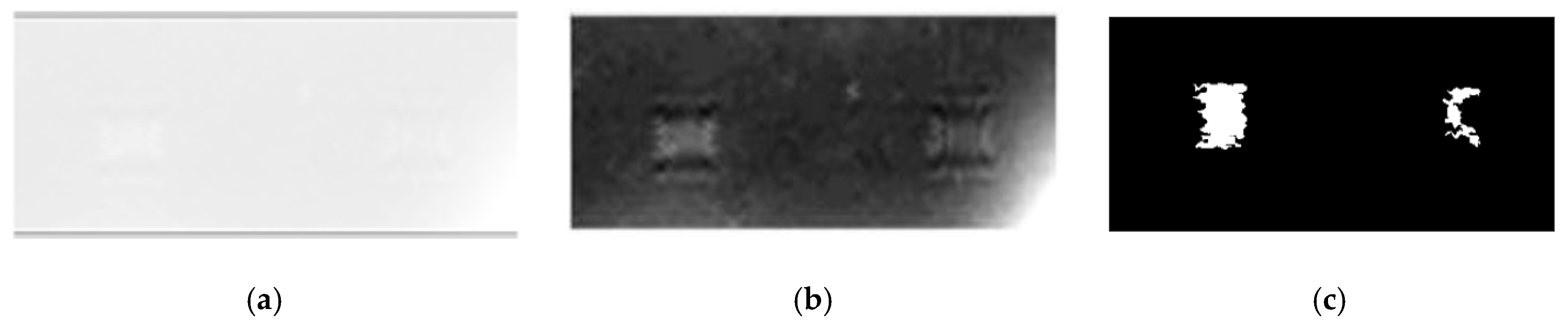
3.1.2.2. Segmentation of Composite Material (SCM) Images

Three algorithms are proposed for this purpose;
Algorithm 1: In the first algorithm, the 2D-FFT, which is one of the most fundamental tools in image analysis and an appropriate candidate for grey level images [37], is computed on CM images. It provides a more precise separation of the desired information than the 1D transform [38]. It can be mathematically formulated as:
Y p + 1 , q + 1 = j = 0 m 1 k = 0 n 1 w m jp w n kq X j + 1 , k + 1
w m = e 2 π i / m
w n = e 2 π i / n
where Y is a discrete Fourier transform, X is a matrix of m × n (2D-image), w m and w n denote complex roots of unity, and i indicates the imaginary unit. The obtained output is shifted to locate the zero-frequency component at the center of the output. The element-wise multiplication of the obtained FFT frequency components with a Wavelet transform is performed to suppress the effect of noise. This convolution was performed one, two, and three times, to investigate its optimization effects on the segmentation results [35]. This process is followed by taking the inverse transform and multi-thresholding to perform segmentation. Finally, the obtained binary image is eroded to remove small objects. This algorithm is summarized as Pseudocode 2.
Pseudocode 2. The proposed FT-based algorithms for defect segmentation in microwave imaging.
Input: Phase and Magnitude
Output: True Target Segmentation
  • Pre-processing of CM images as Section 1.
  • Computation of the 2D-FFT of the on the input microwave image as “y”.
  • Element-wise multiplication of Wavelet transform and “y”.
    for i: 1 to 3 // Separately perform one-, two-, and three-fold convolution
    xy [i] = x*y // Convolution of x and y: (x*y): Integral of the product of the two matrices after one is reversed and shifted.
  • Computation of the inverse Fourier Transform to get the resulting image “I”.
  • Computation of multi-thresholding on “I” to obtain “S” as a segmented image.
  • Performing the morphological operation (erosion) on “S” to remove small objects.
Algorithm 2: The second proposed algorithm, in this section follows the Pseudocode 2 procedure, in which the Wavelet transform function will be replaced by a Gaussian function.
Algorithm 3: The third algorithm is based on fuzzy c-mean (FCM) clustering, followed by Multi-thresholding and erosion. This algorithm has been formed in this paper only for a comparison with Algorithms 1 and 2, as it uses the FCM procedure.

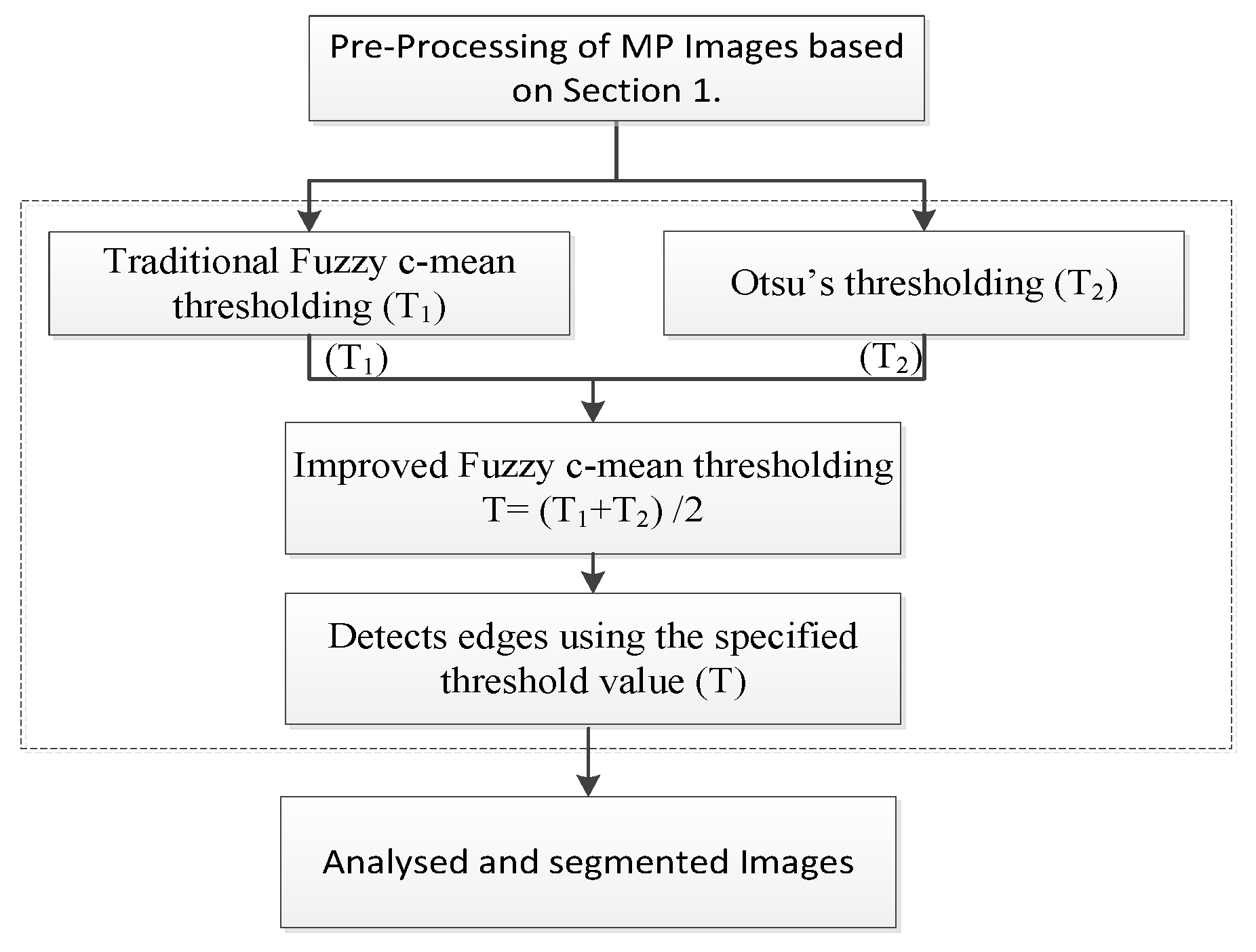
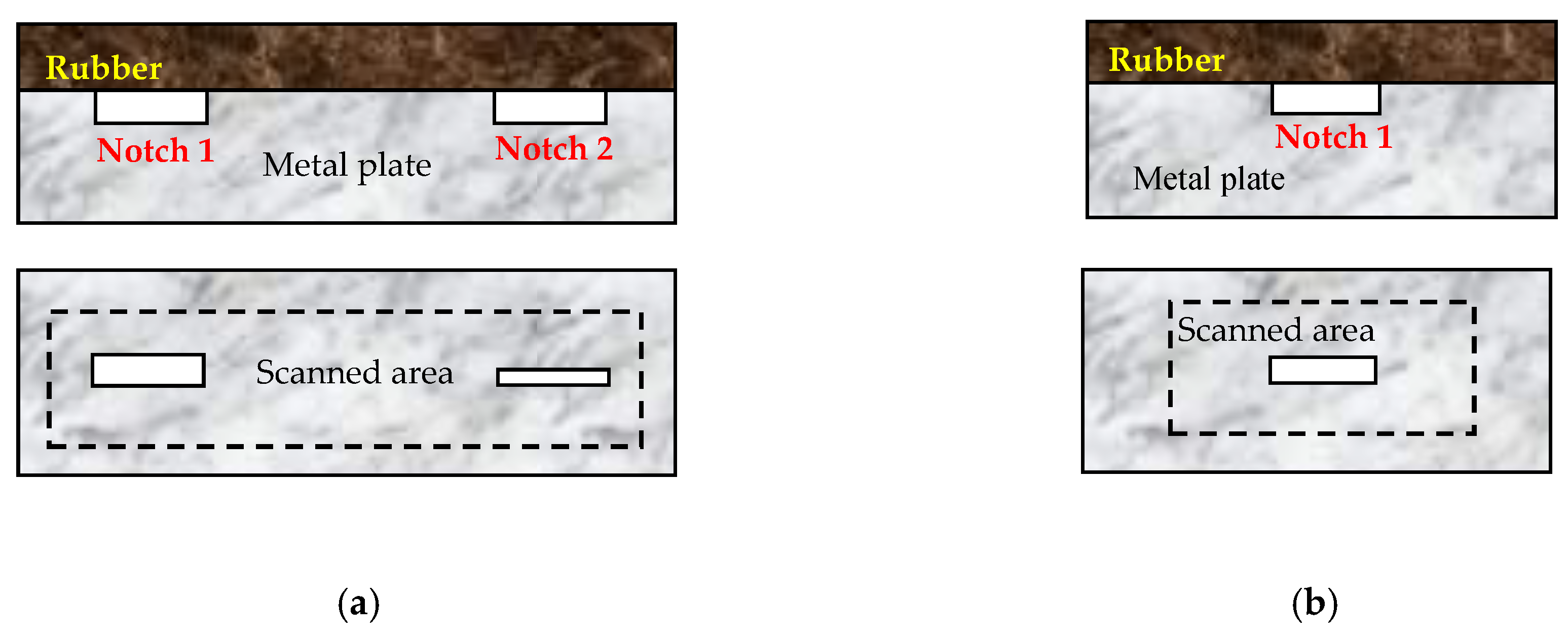
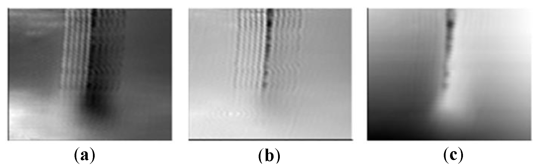
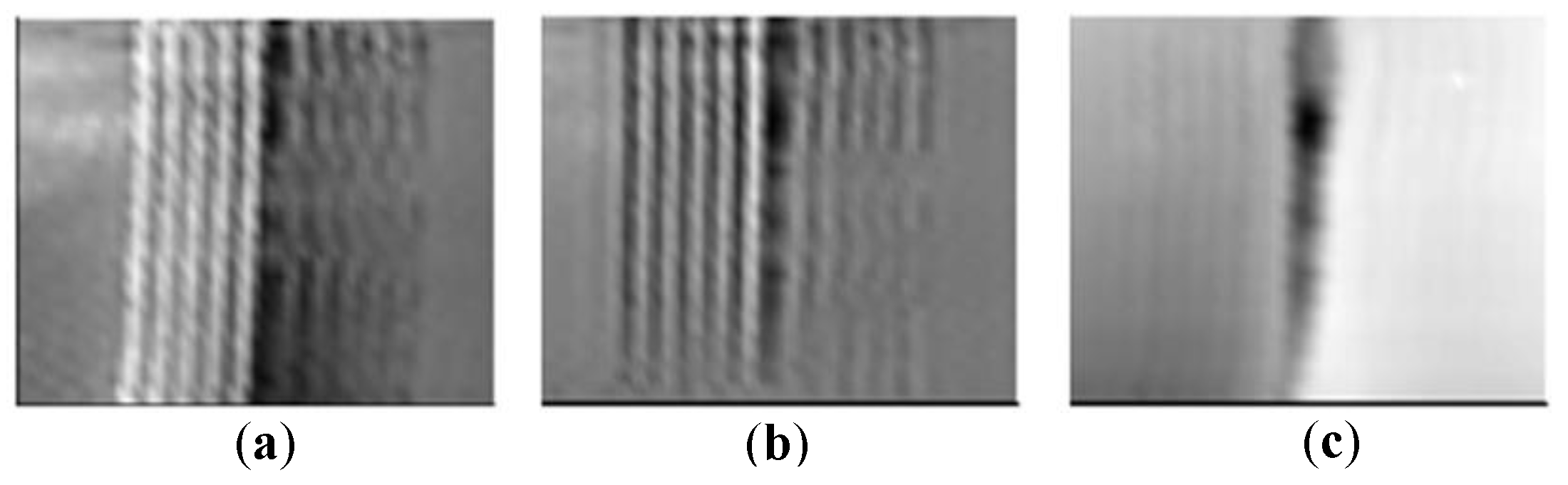
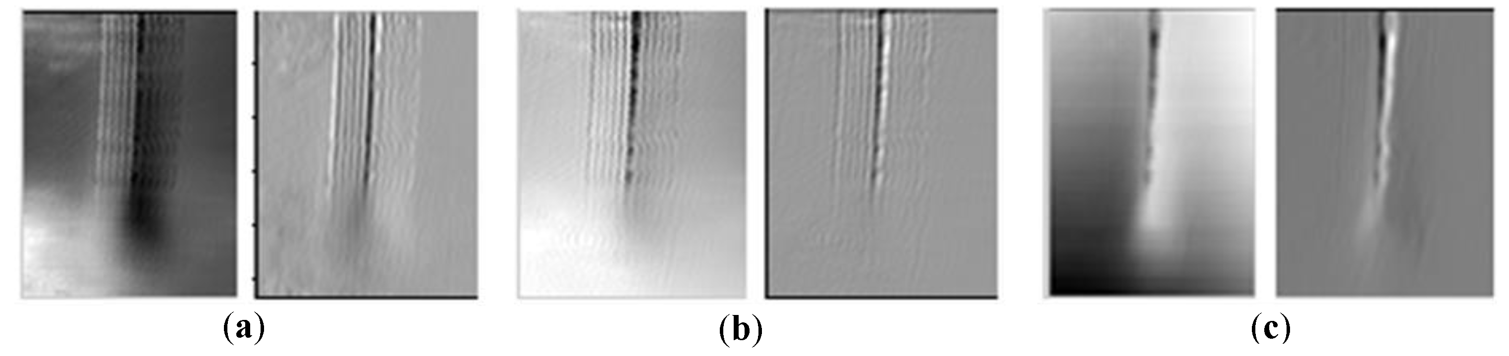
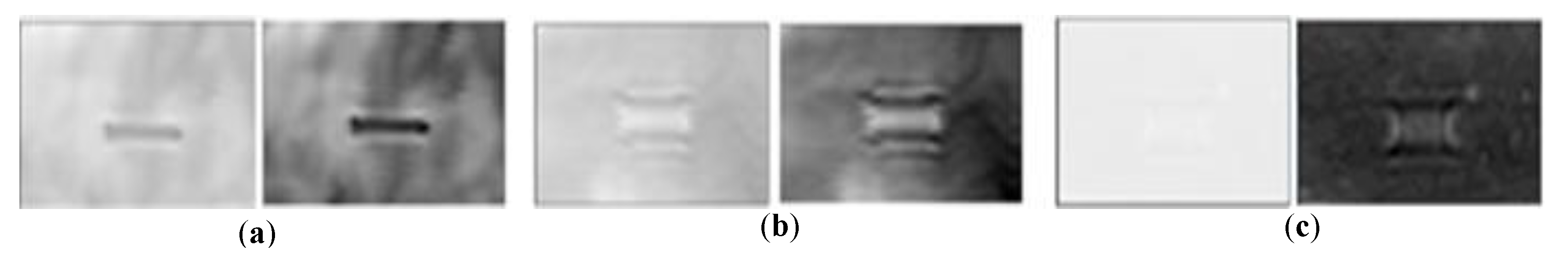
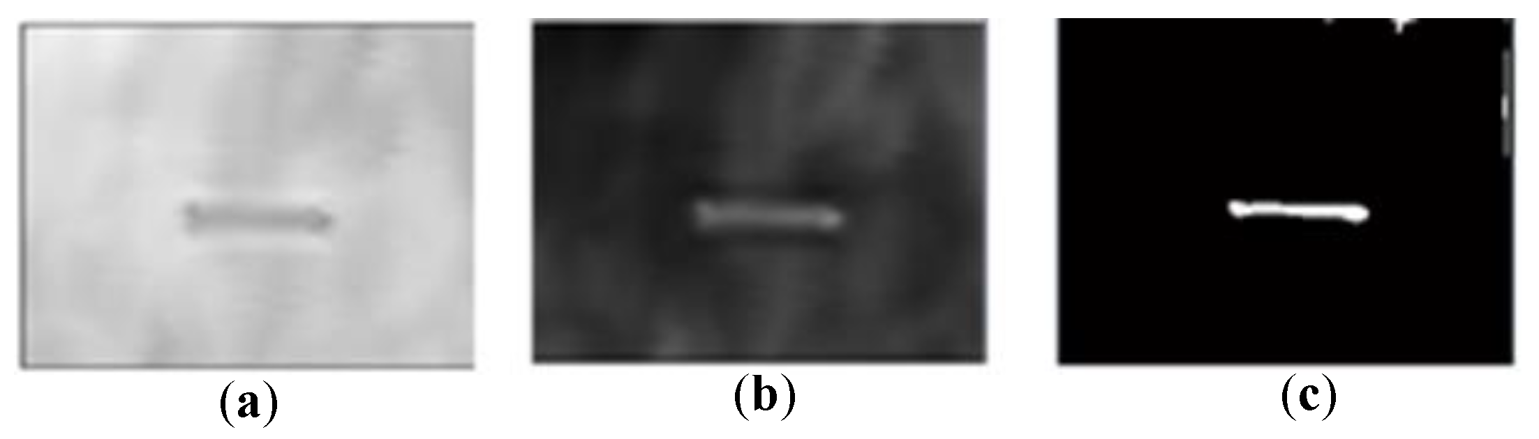
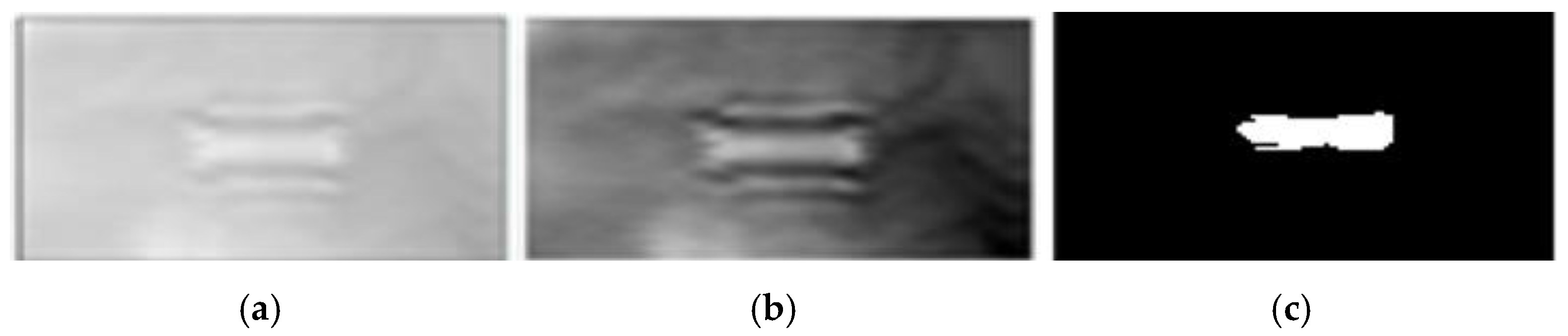
3.1.2.3. Segmentation of Metal Plate (SMP) Images

Three algorithms are proposed for this segmentation. The first and second algorithms almost completely follow the traditional approach, and are investigated for comparison.
Algorithm 1: In the first algorithm, the performance of the traditional gradient magnitude based on Sobel’s gradient operator [36] in the x and y axes is investigated. The edges of the notch were returned at those points where the gradient of the image was at its maximum. Therefore, the edges were achieved by using the Sobel approximation to the derivative.
Algorithm 2: The second algorithm calculates the gradient by using the derivative of a Gaussian filter, and it employs two thresholds; the local maxima of the gradient are considered to be edges.
Algorithm 3: In the third algorithm, the effective selection of the threshold value is performed on pre-processed MP images. The threshold value is obtained by Otsu’s thresholding method, and it is employed, to improve the threshold value of the Fuzzy c-mean technique. The center value of the thresholds was considered to be the desired value, which is more likely to detect true edges. The edges that were not stronger than the threshold value were ignored. Figure 1 shows the flowchart of this algorithm.
The approaches, introduced above, allow experts to accurately visualize the defects that are significantly associated with any subset or linear combination of cracks. The methods can greatly simplify health monitoring in steel, composite materials, and metal structures, respectively. These algorithms can be generalized by investigations on other materials.
In the following section, the experimental setup and results are discussed.

4. Experimental Setup

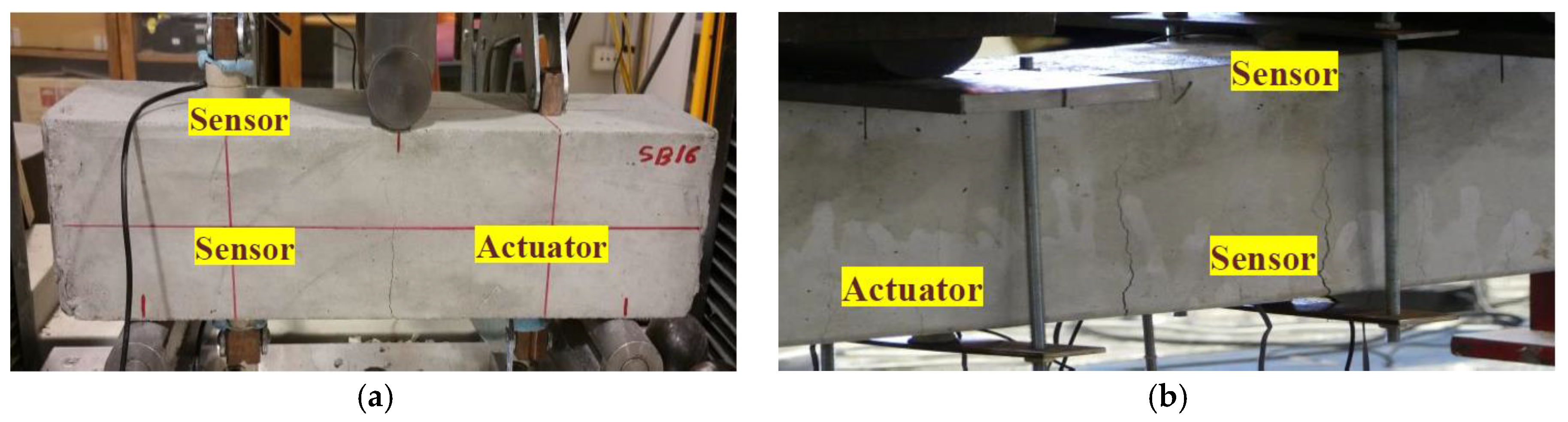
4.1. ML-Based Damage Detection for Concrete and RC Beams

Six concrete beams and four reinforced concrete (RC) beams are fabricated and tested. The 3-point and 4-point bending tests are carried out on beams until failure occurs on the specimens. Table 1 depicts the specifications of our experimental setup.
The size of the concrete beams is 400 mm × 100 mm × 100 mm, with a distance of 200 mm between the sensor and actuator, and the size of the RC beams is 1700 mm × 150 mm × 250 mm, with a distance of 400 mm between the sensor and actuator [39]. An N16 steel bar was used in this experiment as the longitudinal and transverse reinforcement size. The Australian Portland cement type GB, Natural river sand (Fine aggregate), Natural river gravel (Coarse aggregate), and Tap water are used as materials of concrete mixture [39]. The experimental tests are carried out through the Instron high bandwidth system commonly known as the “Universal Test Machine (UTM)”, consisting of a loading cell, for monitoring in real time. Figure 2a,b shows our bending test setup on the beams.

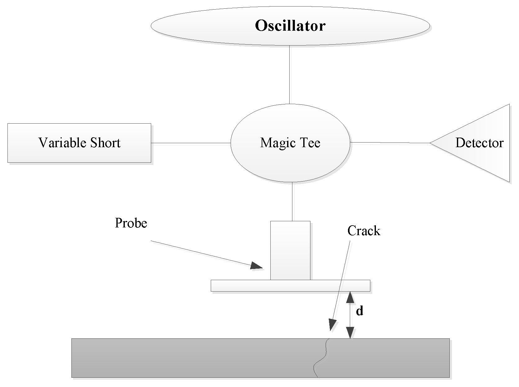
4.2. Microwave Imaging for Damage Detection

The measurement system consisted of a computerized imaging system, including a millimeter-wave reflectometer with a single frequency oscillator, isolator, magic tee, detector, variable short, the OEWA, and a scanning mechanism providing a raster scan of the reflectometer over the sample under test. The open-ended flange-mounted rectangular waveguide probe was used as an open-ended waveguide antenna (OEWA). The OEWAs are robust, reliable, efficient, and relatively simple antennas used for crack detection [10,21,22,23]. The OEWA irradiated the specimen under testing, and picked up the signal reflected from the specimen. This reflected signal was combined with the reference signal in the magic-tee, and the combined data was sent to the detector; the computer recorded its output voltage for every data point over the plane for each specimen. The images were generated through the recorded data in Matlab software, and processed with the proposed image processing algorithms. Figure 3 shows the measurement setup of this study.
To highlight the utility of the single-frequency reflectometer with the OEWA, along with the proposed image processing approaches for imaging different structural materials, various samples were prepared and imaged, as follows.
• Steel Plate
The first specimen was a section of a 12 mm-thick A-36 steel plate with a few through-fatigue cracks that were created during cyclic loading. A W-band open-ended flange-mounted rectangular waveguide probe with aperture dimension of 2.54 mm × 1.27 mm, and with a square (19 mm × 19 mm) flange was used in this investigation. Two scanned areas, with dimensions of 50 mm × 70 mm and 30 mm × 30 mm, included cracks that were obtained at a standoff distance of d ~ 0 mm, d ~ 0.8 mm, and d ~ 1.7 mm.
• Composite Material
The second specimen consisted of six equally thick layers of construction foam with dimensions of 240 mm by 240 mm by 90 mm, as shown in Figure 4a. Four metal discs (each with a diameter of 25 mm and a thickness of 2 mm), in two groups of two, were placed at interfaces between layers 1–2 and 5–6, respectively, as shown in Figure 4. Sample 1 was scanned with a 3 mm step size (along the x- and y-axes), while the complex reflection coefficient was measured at a frequency of 11.5 GHz (X-band) and a 30 mm standoff distance (the distance between the OEWA aperture and the top surface of Sample 1).
• Aluminum Plate
The third specimen consisted of an aluminum plate with dimensions of 150 mm × 60 mm × 10 mm, and was covered by a rubber layer. Two notches were made on the surface of the plate, both with a length of 15 mm and a depth of 1 mm, and with widths of 1 mm and 0.5 mm in notch 1 and notch 2, respectively, as shown in Figure 5. Two scanned areas were made, with dimensions of 40 mm × 20 mm and 100 mm × 40 mm, including notch 1, Figure 5a, and notches 1 and 2, Figure 5b, respectively. The step sizes (sampling) of 1 mm and 0.5 mm along the length and width of the notches, respectively, were used in this investigation.

5. Results and Discussion

5.1. Estimating the Performance Indicator for Traditional and Developed SVM

Experimental data analysis was carried out, considering the signals obtained by SAs mounted on the concrete and RC beams. The signals were recorded every minute throughout the loading period. Table 2 shows the comparative analysis between the traditional and the developed SVM of this study. The classifier learnt from the training features [40] was used to make a decision when the testing data was presented. The performance accuracy was computed through an average of 4-fold cross-validation for 100 runs, and performed for 29 observations. The performance of the algorithms was obtained through computing the average accuracy.
According to the above results, the analysis conducted through an estimation of the performance of the developed SVM obtained an accuracy of 87.22% rather than the traditional SVM, with an accuracy of 84.72%. The suggested method could outperform the benchmark. Further analysis of this performance was carried out by computing the p-value of the T-test, for the average of the accuracies (Table 3).
The obtained p-values in the above cases demonstrate that the difference between the accuracies of the simple SVM and the developed classifier are statistically significant.

5.2. Evaluating the Results of the Proposed SSP Algorithm

This section details an investigation and an analysis of the image results for steel plate sample using the proposed SSP Algorithm in Section 3.1.2.1. The original images herein are 90 GHz images of cracks in a steel plate at different standoff distances with an open-ended waveguide probe. The resulting images were enhanced and segmented at different distances. Figure 6 shows the signals, which were recorded through an open-ended waveguide antenna under 50 × 70 scanning, obtained at three standoff distances of 0 mm, 0.8 mm, and 1.7 mm.
Figure 7 and Figure 8 show the generated images of a crack in Matlab for two scanned areas of 50 × 70 and 30 × 30, with standoff distances of d ~ 0.2, d ~ 0.8 and d ~ 1.7, respectively. As it is evident from Figure 7 and Figure 8, the original images are blurry, and limited information can be obtained.
The first step of the SSP algorithm, as explained before, is to enhance the formed microwave images. Figure 9 shows the enhanced images after performing the enhancement procedure on the original images.
Figure 10 shows the images that were obtained through the employment of the proposed algorithm on the enhanced image (Figure 9), with the gradient magnitude being calculated in six directions of x, y, d1, and d2, followed by Otsu’s thresholding method.
The comparison of the imaging results and the original image, Figure 9 and Figure 10, confirmed that the developed algorithm could identify the crack edges while eliminating noises on the target region. As is evident from the experimental results, the algorithm could provide the image with pure texture and strong edges. Furthermore, Figure 11 shows the 2D grid coordinates that were plotted, based on the coordinates (vectors x and y) of the segmented image. The color change in the middle of grid indicates the occurrence of the abnormality in the data set. The grid-based data representation is an effective way to approximate the amplitude at any location between the grid points.
Table 4 shows the properties of the imaged region, along with the results and descriptions. The results have been computed by using the regionprops () command in MATLAB.

5.3. Evaluating Results for the Proposed SCM Algorithms

This section evaluates results of the proposed SCM Algorithms in Section 3.1.2.2. The original images of the sample for composite material are shown in Figure 12, and they demonstrate that the raw images do not provide much observable information, while four defects exist and must be seen.
To enhance the indications of the desired targets, three proposed algorithms were run using the same condition. The first algorithm was based on one-, two-, and three-fold multiplication of the wavelet transform, with the Fourier transform of the image, followed by the multi-threshold segmentation method and morphological operation “erosion”, to remove the small elements from the image to achieve the target. Figure 13 demonstrates the total process of this segmentation. The first row of images in Figure 13 shows the process as performed by a “single” multiplication of the wavelet and Fourier transform, while the second and third rows show the process as performed by two- and three-fold multiplication of the wavelet and Fourier transform, respectively. However, the obtained result through the single multiplication (row 1), Figure 13d, shows the best result in this section, as it determines three out of four defects, while the other results only detect two defects.
Figure 14 shows the results obtained by the second algorithm. This figure also demonstrates the total process for one-, two- and three-fold multiplication of Gaussian, with the Fourier transform of the image, followed by the multi-threshold segmentation method, and morphological operation “erosion”, to remove the small elements from the image to achieve the target. The first row of images in Figure 14 shows the process performed by a “single” multiplication of the Gaussian and Fourier transform, while the second and third rows of images show the process performed by two- and three-fold multiplications of Gaussian and Fourier transforms, respectively. However, the results obtained through two-fold multiplication (Figure 14d, row 2) shows the best-segmented result, in this section, as it determines four out of four defects, with less noise than the other results in Figure 14.
Figure 15 shows the results that are obtained through the Algorithm 3. This figure also shows the total process of target segmentation using fuzzy c-mean clustering, followed by Multi-thresholding and erosion with two different sizes, 10 and 15, of the structuring element. The results show that the higher size of the structuring element makes the image cleaner, but they change the detected defects sequentially, and make the image unreal. However, the obtained result in Figure 15d shows the best-segmented result; in this section, as it determines three out of four defects and the skeleton of the fourth defect.
The comparison of segmentation results using the above three algorithms shows that the results achieved by “Algorithm 2”, Figure 14, outperform the other two algorithms. In Figure 14, the best demonstration is for the “two-fold multiplication of Gaussian with the Fourier transform” which is followed by a multi-threshold segmentation method and morphological operation “erosion” (Figure 14, row 2b). The image shows a clear view of four separated defects with less noise and redundant objects.
Also, this section presents the surface plots for the magnitude and phase of reconstructed images as a further comparison of Algorithms 1 and 2. Figure 16a shows the surface plot for the wavelet transform basis and Fourier transform (Algorithm 1). The plots in the first row of Figure 16a demonstrate the magnitude and phase of the 2D data, containing random phases. The plots in the second row of Figure 16 demonstrate the magnitude and phase of the 2D data containing random magnitudes. Figure 16b presents the surface plots for the magnitude and phase of a reconstructed image, based on Gaussian filtering and Fourier transform (Algorithm 2).
The comparison of Figure 16a,b shows that the basis had little effect on the phase, while the magnitude changed from [0,0.03] in Figure 16a to [0,1] in Figure 16b, which demonstrates the better performance of the second algorithm over the other algorithm. Figure 17 shows the results obtained from the setup on Figure 5b.
Both the proposed Algorithms 1 and 2 show almost similar results (rows 1 and 2), while they outperformed the Fuzzy c-mean algorithm (row 3). As is obvious from the Figure 17 (row 3a), Figure 17 (row 3b), and Figure 17 (row 3c), the outcome of FCM is dependent on the selection of the threshold value. The threshold value of the first figure is 0.206500, while the second and third figures have threshold values of 0.211538 and 0.480769, respectively.
From all of the above results obtained through employing the algorithms on experimental setups in Figure 5a,b, it is concluded that the proposed algorithms were successfully adapted to determine the notch regions. However, the algorithms discriminated the boundaries of the notches, where Algorithm 3 (benchmark) was less successful (Figure 16, row 3a).

5.4. Evaluating Results for the Proposed SMP Algorithms

This section evaluates results of the proposed SMP Algorithms in Section 3.1.2.3. Figure 18 show the original (left) and enhanced (right) images of notch 1 under the 2 mm-thick rubber layer, obtained at three standoff distances of 0.1 mm, 0.25 mm, and 4 mm. As is evident from Figure 18, the original images (left) were blurry, and no information could be gained from the images of notches under the 2 mm-thick rubber layer with a standoff distance of 4 mm, as shown in Figure 18c. However, the right-hand-side images show the results of image enhancement over the original images. It is obvious that the enhanced images can show up the existence of notches.
Figure 19 shows the original and enhanced image of notches 1 and 2 under the 4 mm-thick rubber layer obtained at a standoff distance of 0.1 mm. As is evident from Figure 19a, the original image was blurred, and no information could be gained from an image with a standoff distance of 0.1 mm, while the notches were clearly observable on the enhanced images (Figure 19b).
By applying the image-enhancement algorithm, the notches in the specimens became clear, as shown in Figure 18 (a(right), b(right), c(right)), and Figure 19b, thus meeting one of the goals of this investigation. In order to make progress with the algorithms, the enhanced image of notch 1, Figure 18a, was used to apply three image processing algorithms, as presented in the Section 3.1.2. To save space, the corresponding images obtained for Figure 18b,c after the SCM process, are provided in Appendix A. Figure 20 shows the images obtained for notch 1 in each step of Algorithm 1.
Figure 21 shows the images obtained for notch 1 in each step of Algorithm 2.
Figure 22 shows the images obtained for notch 1 in each step of Algorithm 3. In order to facilitate the discussion, in Algorithm 3, the developed Fuzzy c-mean thresholding algorithm was applied, to segment the image. However, the obtained threshold value was 2.05 × 10⁻¹, while for Otsu’s thresholding method and the traditional fuzzy-c-mean thresholding algorithm, it was 1.7 × 10⁻¹ and 2.4 × 10⁻¹, respectively.
Figure 23 shows the comparison of the segmented images of notch 1, obtained with Algorithms 1–3. According to the segmented images, the developed Fuzzy c-mean thresholding algorithm (Algorithm 3) outperformed the other two algorithms. As is evident from Figure 23c, the true edges, which were detected by the developed Fuzzy c-mean thresholding algorithm, were more accurate with less noise, while Figure 23a,b include redundant edges and noises, which represent the segmentation error.
A further investigation of the developed algorithm was carried out, by comparing its performance with the traditional Fuzzy c-mean thresholding algorithm and Otsu’s thresholding algorithm. Figure 24 depicts this comparison. However, the obtained results show that the developed Fuzzy c-mean thresholding algorithm performed better than the other two traditional algorithms. To save space, the obtained corresponding segmented results with respect to a proposed algorithm have been provided in Appendix A.
Imaging results confirmed that the developed Fuzzy c-mean thresholding algorithm can identify the notch edges while eliminating the noises on the target region, which proves that the algorithm could achieve the images with pure textures and strong edges.

6. Conclusions

This paper first proposed a damage detection algorithm, using the developed ML approaches for concrete and RC beams, and then investigated the performance of microwave imaging on the local detection and visualization of damage in a steel plate, a composite material, and a metal plate. The SVM-based algorithm was developed and compared with traditional SVM, through the response data of various numbers of specimens mounted on SAs, to validate its effectiveness. Accuracy and a t-test were used for this validation. The proposed algorithm outperformed the performance of traditional SVM. It can be concluded that the extraction of subsequent knowledge from the training phase, and its fusion with unsupervised machine learning (k-nearest neighbor), can help to improve the performance of traditional SVM.
Then, the microwave- and millimeter-wave imaging approach was used as the second approach of this paper. The obtained images had a very low resolution, and in some cases, no information was observable. The images were processed through different proposed image-processing algorithms. The algorithms were based on the Fourier transform, Wavelet transform, Fuzzy c-mean, Gaussian filter, Median filter, and Gradient magnitude. The proposed algorithms made it possible for clear observations of anomalous occurrences in structures to be made. The results prove that the algorithms have the potential to successfully enhance microwave images with poor resolution, and to identify areas of interest, specifically in structural health monitoring.
The purpose of this study was to minimize the need for manual inspections of civil structures, and it sought to complement edge-based damage detection methods for hazardous scenarios. However, the proposed algorithms of this study can be applied to different imaging applications where the enhancement of quality, and obtaining the area of interest are critical approaches.

Author Contributions

Methodology, A.N.H.; Conceptualization, B.S. and R.L. and M.R.; Supervision, B.S., R.L. and S.K.; Writing-Review & Editing, A.N.H., R.L., M.R. and B.S.; Resources, S.K.

Funding

This research received no external funding.

Acknowledgments

The authors acknowledge the intellectual contribution of the late Sergey Kharkovsky of the Centre for Infrastructure Engineering on the electromagnetic imaging part of this work.

Conflicts of Interest

The authors declare no conflict of interest

Appendix A

Additional Enhancement and Segmentation Results of proposed algorithms.
Figure A1. Images of notch 1 under the 2 mm-thick rubber layer obtained at a standoff distance of 0.25 mm: (a) original, and after (b) average filtering and (c) thresholding by the developed fuzzy c-mean thresholding algorithm.
Applsci 09 02810 g0a1
Figure A2. Images of notch 1 under the 2 mm-thick rubber layer obtained at a standoff distance of 4 mm: (a) original and after (b) average filtering and (c) thresholding by the developed fuzzy c-mean thresholding algorithm.
Applsci 09 02810 g0a2
Figure A3. Images of notches 1 and 2 under the 4-mm thick rubber layer obtained at a standoff distance of 0.1 mm: (a) original and after (b) average filtering and (c) thresholding by the developed fuzzy c-mean thresholding algorithm.
Applsci 09 02810 g0a3

References

  1. Schmerr, L.W. Fundamentals of Ultrasonic Nondestructive Evaluation: A Modeling Approach; Springer: New York, NY, USA, 2013. [Google Scholar]
  2. Abdel-Qader, I.; Abudayyeh, O.; Kelly, M. Analysis of Edge-Detection Techniques for Crack Identification in Bridges. J. Comput. Civ. Eng. 2003, 17, 255–263. [Google Scholar] [CrossRef]
  3. Salehi, H.; Das, S.; Chakrabartty, S.; Biswas, S.; Burgueño, R. Structural Assessment and Damage Identification Algorithms Using Binary Data. In Proceedings of the ASME 2015 Conference on Smart Materials, Adaptive Structures and Intelligent Systems, Colorado Springs, CO, USA, 21–23 September 2015; p. V002T05A011. [Google Scholar]
  4. Yuvaraj, P.; Murthy, A.R.; Iyer, N.R.; Samui, P.; Sekar, S.K. Prediction of fracture characteristics of high strength and ultra high strength concrete beams based on relevance vector machine. Int. J. Damage Mech. 2014, 23, 979–1004. [Google Scholar] [CrossRef]
  5. Chou, J.-S.; Pham, A.-D. Hybrid computational model for predicting bridge scour depth near piers and abutments. Autom. Constr. 2014, 48, 88–96. [Google Scholar] [CrossRef]
  6. Das, S.K.; Samui, P.; Sabat, A.K. Application of Artificial Intelligence to Maximum Dry Density and Unconfined Compressive Strength of Cement Stabilized Soil. Geotech. Geol. Eng. 2011, 29, 329–342. [Google Scholar] [CrossRef]
  7. Worden, K.; Lane, A.J. Damage identification using support vector machines. Smart Mater. Struct. 2001, 10, 540. [Google Scholar] [CrossRef]
  8. Bornn, L.; Farrar, C.R.; Park, G.; Farinholt, K. Structural Health Monitoring with Autoregressive Support Vector Machines. J. Vib. Acoust. 2009, 131, 021004–021004-9. [Google Scholar] [CrossRef]
  9. Kim, Y.; Chong, J.W.; Chon, K.H.; Kim, J. Wavelet-based AR–SVM for health monitoring of smart structures. Smart Mater. Struct. 2013, 22, 015003. [Google Scholar] [CrossRef]
  10. Zoughi, R.; Kharkovsky, S. Microwave and millimetre wave sensors for crack detection. Fatigue Fract. Eng. Mater. Struct. 2008, 31, 695–713. [Google Scholar]
  11. Kharkovsky, S.; Case, J.T.; Ghasr, M.T.; Zoughi, R.; Bae, S.W.; Belarbi, A. Application of microwave 3D SAR imaging technique for evaluation of corrosion in steel rebars embedded in cement-based structures. In Proceedings of the AIP Conference Proceedings, Philadelphia, PA, USA, 1–2 August 2012; Volume 1430, pp. 516–1523. [Google Scholar]
  12. Kharkovsky, S.; Giri, P.; Samali, B. Non-contact inspection of construction materials using 3-axis multifunctional imaging system with microwave and laser sensing techniques. {IEEE} Instrum. Meas. Mag. 2016, 19, 6–12. [Google Scholar] [CrossRef]
  13. Flood, I.; Christophilos, P. Modeling construction processes using artificial neural networks. Autom. Constr. 1996, 4, 07–320. [Google Scholar] [CrossRef]
  14. Tran, H. A hybrid fuzzy inference model based on RBFNN and artificial bee colony for predicting the uplift capacity of suction caissons. Autom. Constr. 2014, 41, 60–69. [Google Scholar]
  15. Faghih, N.M.; Rezaei, J.; Tavakoli, B.A.M. Efficiency Evaluation of Health Services using Linear Programming. J. Sch. Public. Health Inst. Public. Health Res. 2009, 7, 25–35, [In Persian]. [Google Scholar]
  16. Feng, M.Q.; Roqueta, G.; Jofre, L. 22—Non-Destructive Evaluation (NDE) of Composites: Microwave Techniques. In Non-Destructive Evaluation (NDE) of Polymer Matrix Composites; Karbhari, V.M., Ed.; Woodhead Publishing: Sawston, UK, 2013; pp. 574–616. [Google Scholar]
  17. Castro, A.F.; Valcuende, M.; Vidal, B. Using microwave near-field reflection measurements as a non-destructive test to determine water penetration depth of concrete. NDT E Int. 2015, 75, 26–32. [Google Scholar] [CrossRef]
  18. Buttress, A.; Jones, A.; Kingman, S. Microwave processing of cement and concrete materials—Towards an industrial reality? Cem. Concr. Res. 2015, 68, 112–123. [Google Scholar] [CrossRef]
  19. Yan, A.; Wu, K.; Zhang, X. A quantitative study on the surface crack pattern of concrete with high content of steel fiber. Cem. Concr. Res. 2002, 32, 1371–1375. [Google Scholar] [CrossRef]
  20. Rashidi, M.; Ghodrat, M.; Samali, B.; Kendall, B.; Zhang, C. Remedial modelling of steel bridges through application of analytical hierarchy process (AHP). Appl. Sci. 2017, 7, 168. [Google Scholar] [CrossRef]
  21. Kharkovsky, S.; Zoughi, R. Microwave and millimeter wave nondestructive testing and evaluation—Overview and recent advances. IEEE Instrum. Meas. Mag. 2007, 10, 26–38. [Google Scholar] [CrossRef]
  22. Kharkovsky, S.; Ghasr, M.T.; Zoughi, R. Near-Field Millimeter-Wave Imaging of Exposed and Covered Fatigue Cracks. IEEE Trans. Instrum. Meas. 2009, 58, 2367–2370. [Google Scholar] [CrossRef]
  23. Zoughi, R. Microwave Non-Destructive Testing and Evaluation Principles; Springer Science & Business Media: Berlin, Germany, 2000. [Google Scholar]
  24. Ahanian, I.; Sadeghi, S.H.H.; Moini, R. An array waveguide probe for detection, location and sizing of surface cracks in metals. NDT E Int. 2015, 70, 38–40. [Google Scholar] [CrossRef]
  25. Noori Hoshyar, A.; Kharkovsky, S.N.; Samali, B.; Zoughi, R. Millimeter wave imaging of notches in metal specimens under dielectric coating using image processing. In Proceedings of the Fourth Conference On Smart Monitoring, Assessment And Rehabilitation Of Civil Structures, Zurich, Switzerland, 13–15 September 2017. [Google Scholar]
  26. Moosazadeh, M.; Kharkovsky, S.; Case, J.T. Microwave and millimetre wave antipodal Vivaldi antenna with trapezoid-shaped dielectric lens for imaging of construction materials. IET Microw. Antennas Propag. 2016, 10, 301–309. [Google Scholar] [CrossRef]
  27. McAndrew, A. Introduction to Digital Image Processing with MATLAB; Course Technology: Cambridge, MA, USA, 2004. [Google Scholar]
  28. Vapnik, V.N. An overview of statistical learning theory. IEEE Trans. Neural Networks 1999, 10, 988–999. [Google Scholar] [CrossRef] [PubMed]
  29. Maali, Y.; Al-Jumaily, A. Self-advising support vector machine. Knowl. Based Syst. 2013, 52, 214–222. [Google Scholar] [CrossRef]
  30. Lauer, F.; Bloch, G. Incorporating prior knowledge in support vector machines for classification: A review. Neurocomputing 2008, 71, 1578–1594. [Google Scholar] [CrossRef] [Green Version]
  31. Zhan, Y.; Shen, D. An adaptive error penalization method for training an efficient and generalized SVM. Pattern Recogn. 2006, 39, 342–350. [Google Scholar] [CrossRef]
  32. Hoshyar, A.; Kharkovsky, S.; Samali, B. Statistical Features and Traditional SA-SVM Classification Algorithm for Crack Detection. J. Signal Inf. Process. 2018, 9, 111–121. [Google Scholar] [CrossRef] [Green Version]
  33. Hoshyar, A.N.; Kharkovsky, S.; Taghavipour, S.; Samali, B.; Liyanapathirana, R. Structural Damage Detection of a Concrete Based on the Autoregressive All-pole Model Parameters and Artificial Intelligence Techniques. In Proceedings of the 9th International Conference on Signal Processing Systems, Auckland, New Zealand, 27–30 November 2017; pp. 57–61. [Google Scholar]
  34. Günther Wyszecki, W.S.S. Color Science: Concepts and Methods, Quantitative Data and Formulae; Wiley-Interscience: Hoboken, NJ, USA, 1982; p. 968. [Google Scholar]
  35. Hoshyar, A.N.; Kharkovsky, S.; Samali, B. Microwave imaging of composite materials using image processing. In Proceedings of the 2015 International Symposium on Antennas and Propagation (ISAP), Hobart, Tasmania, Australia, 9–12 November 2015. [Google Scholar]
  36. Gonzalez, R.C.; Woods, R.E.; Eddins, S.L. Digital Image Processing Using MATLAB, 2nd ed.; Gatesmark Publishing: Knoxville, TN, USA, 2009. [Google Scholar]
  37. Grigoryan, A.M.; Agaian, S.S. Tensor transform-based quaternion fourier transform algorithm. Inf. Sci. 2015, 320, 62–74. [Google Scholar] [CrossRef]
  38. Bone, D.J.; Bachor, H.A.; Sandeman, R.J. Fringe-pattern analysis using a 2-D Fourier transform. Appl. Opt. 1986, 25, 1653–1660. [Google Scholar] [CrossRef]
  39. Noori Hoshyar, A.; Samali, B.; Liyanapathirana, R.; Taghavipour, S. Analysis of failure in concrete and reinforced-concrete beams for the smart aggregate–based monitoring system. Struct. Health Monit. 2019. [Google Scholar] [CrossRef]
  40. Aggelis, D.G. Classification of cracking mode in concrete by acoustic emission parameters. Mech. Res. Commun. 2011, 38, 153–157. [Google Scholar] [CrossRef]
Figure 1. Flowchart of the developed Fuzzy c-mean thresholding algorithm.
Applsci 09 02810 g001
Figure 2. Bending test set up: (a) concrete, (b) RC beam.
Applsci 09 02810 g002
Figure 3. Measurement setup.
Applsci 09 02810 g003
Figure 4. (a) Picture and schematic of (b) the top view, with the embedded disks indicated, (c) the cross-sectional side view at Plane 1, and (d) the cross-sectional side view at Plane 2.
Applsci 09 02810 g004
Figure 5. Cross-sectional side view (upper) and schematic of the top view without the rubber layer (lower) of the parts of aluminum plate with (a) notch 1 and (b) notches 1 and 2.
Applsci 09 02810 g005
Figure 6. Signals recorded under 50 × 70 scanning, obtained at three standoff distances: (a) 0.2 mm, (b) 0.8 mm, and (c) 1.7 mm.
Applsci 09 02810 g006
Figure 7. Original images of the portion of the covered crack under 50 × 70 scanning, obtained at three standoff distances: (a) 0.2 mm, (b) 0.8 mm, and (c) 1.7 mm.
Applsci 09 02810 g007
Figure 8. Original images of the portion of the covered crack under 30 × 30 scanning, obtained at three standoff distances: (a) 0.2 mm, (b) 0.8 mm, and (c) 1.7 mm.
Applsci 09 02810 g008
Figure 9. (a) Left: Original image with d ~ 1.7, (a) Right: Enhanced image with d ~ 1.7, (b) Left: Original image with d ~ 0.8, (b) Right: Enhanced image with d ~ 0.8 (c) Left: Original image with d ~ 0.2, (c) Right: Enhanced image with d ~ 0.2 mm.
Applsci 09 02810 g009
Figure 10. (a) Gradient in the x-direction (b) Gradient in the y-direction (c) Gradient in the d1 direction, (d) Gradient in the d2 direction, (e) Gradient magnitude, (f) Otsu’s thresholding.
Applsci 09 02810 g010
Figure 11. 2D grid coordinates of segmented image.
Applsci 09 02810 g011
Figure 12. Microwave image of the sample for the composite material: (a) magnitude and (b) phase.
Applsci 09 02810 g012
Figure 13. The total process of target segmentation of the sample, using Fourier transform and Wavelet transform, followed by Multi-thresholding and erosion, with (1) single, (2) two-fold, and (3) three-fold multiplications, (a) Fourier transforms, (b) inverted Fourier transforms (magnitude), (c) inverted Fourier transforms (phase), and (d) segmented results.
Applsci 09 02810 g013
Figure 14. The total process of target segmentation of sample using Fourier transform and Gaussian followed by Multi-thresholding and erosion, with (1) single-, (2) two-fold, and (3) three-fold multiplications, (a) Fourier transforms, (b) inverted Fourier transforms (magnitude), (c) inverted Fourier transforms (phase), and (d) segmented results.
Applsci 09 02810 g014
Figure 15. Images of the sample, showing the total process of target segmentation, using fuzzy c-mean clustering, followed by multi-thresholding and erosion, (a) original image, (b) fuzzy c-mean clustering, (c) erosion by structuring element object 10, and (d) erosion by structuring element object 15.
Applsci 09 02810 g015
Figure 16. 3D demonstration of the phase and magnitude of the 2D data, (a) a reconstructed image based on a wavelet transform, and (b) a reconstructed image based on a Gaussian transform.
Applsci 09 02810 g016
Figure 17. The total process of target segmentation using (1) Fourier transform and Wavelet transform, followed by multi-thresholding and erosion, (2) Fourier transform and Gaussian, followed by multi-thresholding and erosion, (a) Fourier transforms, (b) inverted Fourier transforms (magnitude), (c) inverted Fourier transforms (phase), and (d) segmented results, and (3) a fuzzy c-mean algorithm with, (a) a threshold value of 0.206500, (b) a threshold value of 0.211538, and (c) a threshold value of 0.480769.
Applsci 09 02810 g017
Figure 18. Original (left) and enhanced (right) images of notch 1 under the 2 mm-thick rubber layer, obtained at three standoff distances: (a) 0.1 mm, (b) 0.25 mm, and (c) 4 mm.
Applsci 09 02810 g018
Figure 19. The (a) original and (b) enhanced images of notches 1 and 2 under the 4 mm-thick rubber layer, obtained at a standoff distance of 0.1 mm.
Applsci 09 02810 g019
Figure 20. Images of notch 1 under the 2 mm-thick rubber layer obtained at a standoff distance of 0.1 mm: (a) original and after (b) average filtering, (c) gradient filtering in the x-direction ( G x ) , (d) gradient filtering in the y-direction ( G y ) and (e) gradient magnitude with the Sobel method, | G | = G x 2 + G y 2 .
Applsci 09 02810 g020
Figure 21. Images of notch 1 under the 2 mm-thick rubber layer: (a) original and after (b) average filtering, (c) the canny edge detection algorithm obtained at a standoff distance of 0.1 mm.
Applsci 09 02810 g021
Figure 22. Images of notch 1 under the 2 mm-thick rubber layer obtained at a standoff distance of 0.1 mm: (a) original and after (b) average filtering, and (c) thresholding by the developed fuzzy c-mean thresholding algorithm.
Applsci 09 02810 g022
Figure 23. Notch edge detection, obtained with the (a) gradient magnitude, using Sobel’s gradient, (b) Canny edge detection algorithm, and (c) the developed fuzzy c-mean thresholding algorithm.
Applsci 09 02810 g023
Figure 24. Notch edge detection, obtained with (a) the developed fuzzy c-mean thresholding algorithm, (b) the traditional fuzzy c-mean thresholding algorithm, and (c) Otsu’s thresholding algorithm.
Applsci 09 02810 g024
Table 1. Specifications for experimental setup.
Concrete BeamSize (mm)Loading Capacity (kN)Displacement Movement (mm/min)Loading Cell Starting Point
Simple400 × 100 × 100 200 0.01 0
Reinforced 1700 × 150 × 2501000 0.009 0
Table 2. Comparison of accuracy between the traditional and the developed Support Vector Machine (SVM).
Accuracy (%)
No. ObservationsConcrete BeamRC Beam
Simple SVMDeveloped SVM Simple SVMDeveloped SVM
184.7287.2385.2686.19
284.6387.1985.4287.14
384.8187.2285.3986.19
484.7687.2385.486.18
584.8387.1985.3986.15
684.4687.2385.2886.19
784.9187.2285.286.5
884.6387.2485.4886.19
984.6587.3585.486.19
1084.6187.2285.5286.56
1184.9187.285.3886.25
1284.5287.1885.2986.19
1384.6687.285.4386.66
1484.8787.2185.2986.16
1584.887.2185.4286.18
1684.8187.1985.4686.19
1784.8287.2385.4486.12
1884.5887.2385.3186.19
1984.8887.2285.2786.19
2084.7687.2385.4486.21
2184.5587.2385.3286.19
2284.887.2885.4386.38
2384.6587.1985.3286.19
2484.687.1785.3786.19
2584.8787.1985.4786.47
2684.5887.2285.4586.19
2784.8387.2285.2486.72
2884.9387.3585.4286.14
2984.6887.1985.486.19
Average84.7287.2285.3886.29
Table 3. T-Test: Simple SVM and developed SVM sample for the means.
Simple SVMDeveloped SVM
Mean84.7387.22
Observations2929
t statistic−101.443
P (T ≤ t), one-tailed8.78×10−3
P (T ≤ t) two-tail1.76×10−3
Table 4. Properties of the image region, results, and descriptions.
PropertyResultDescription
Centroid[38.7045 27.9205]Mass center of the region
BoundingBox[35.5000 2.5000 7 64]Smallest rectangle containing the region
FilledImage[64 × 7 logical]Image with the size of bounding box for the region
FilledArea176Number of ‘on’ pixels
MajorAxisLength68.7051Number of pixels for the major axis of the ellipse
MinorAxisLength5.8664Number of pixels for the minor axis of the ellipse
Orientation88.0654 (degree)Angle between the MajorAxisLength and the x-axis

