A Short-Term Forecast Model of foF2 Based on Elman Neural Network


Abstract
:1. Introduction
2. Model Principle
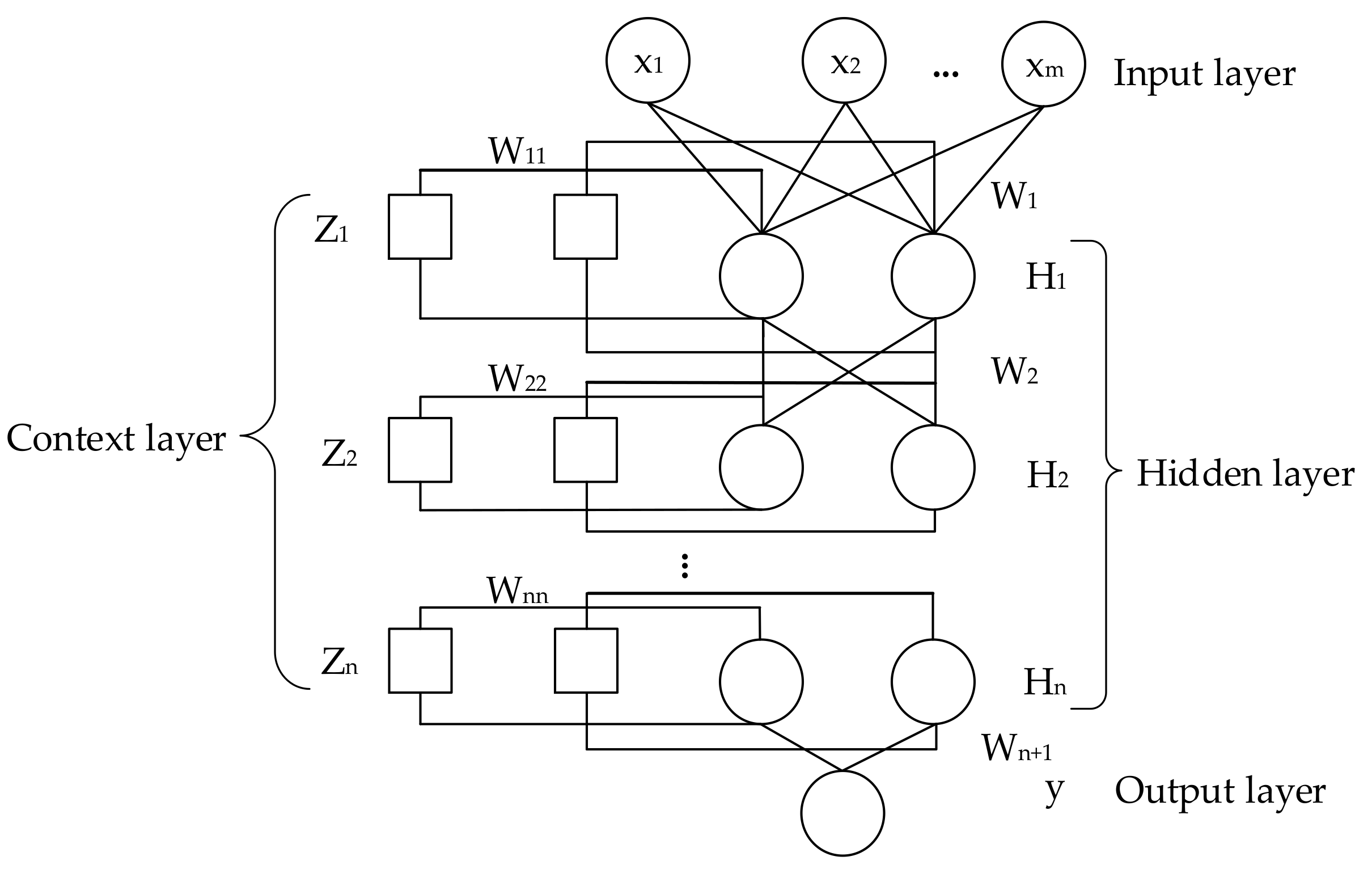
2.1. Elman Neural Network (ENN)
2.2. Improved Particle Optimization Algorithm
2.2.1. Particle Swarm Optimization for ENN
2.2.2. Improvement of Particle Swarm Optimization
3. Data Settings and Model Construction
3.1. Setting of Training Data
3.1.1. Diurnal and Seasonal Variation
3.1.2. Solar and Magnetic Activities
3.1.3. Present Value of foF2
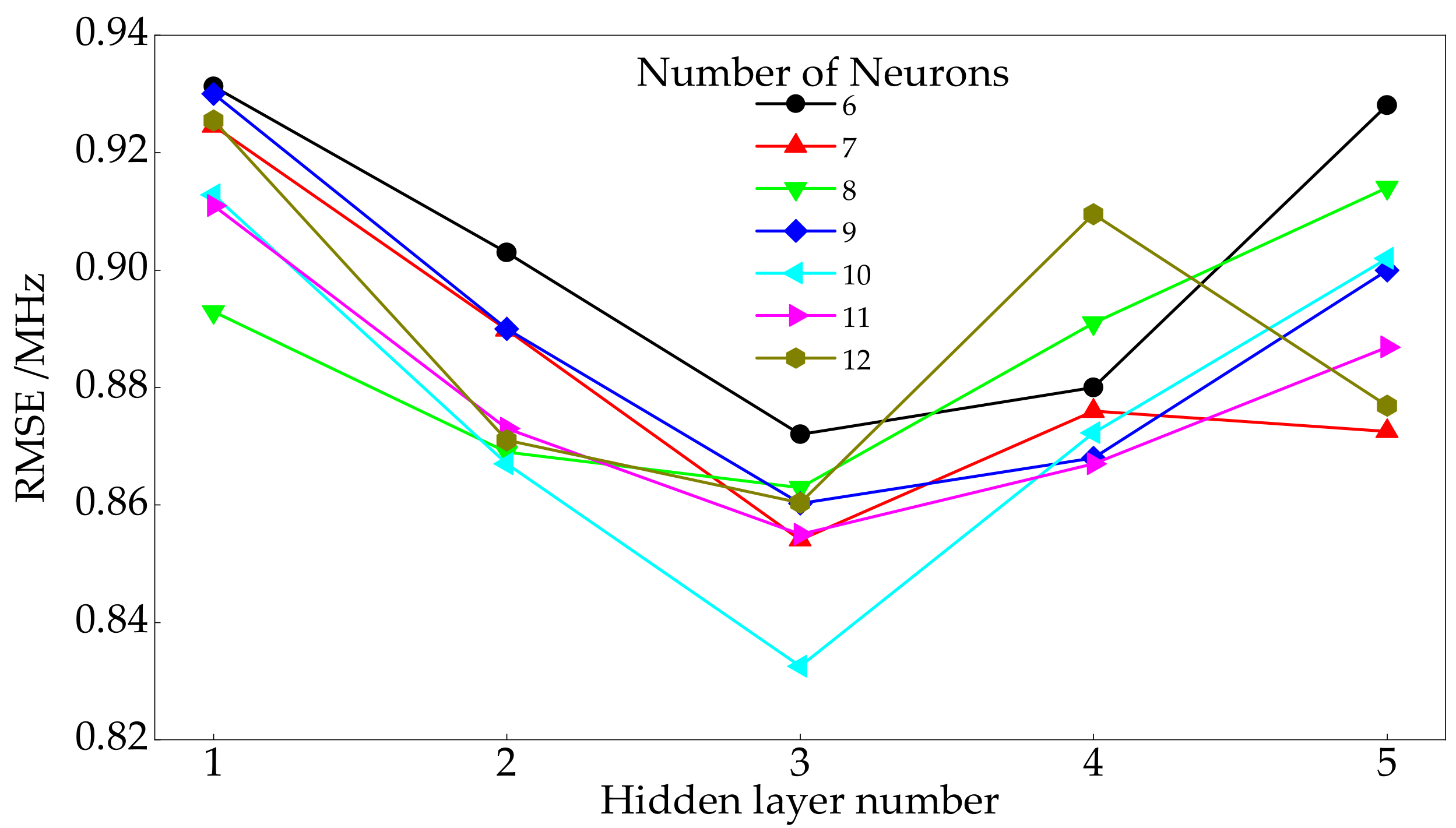
3.2. Architecture of the ENN
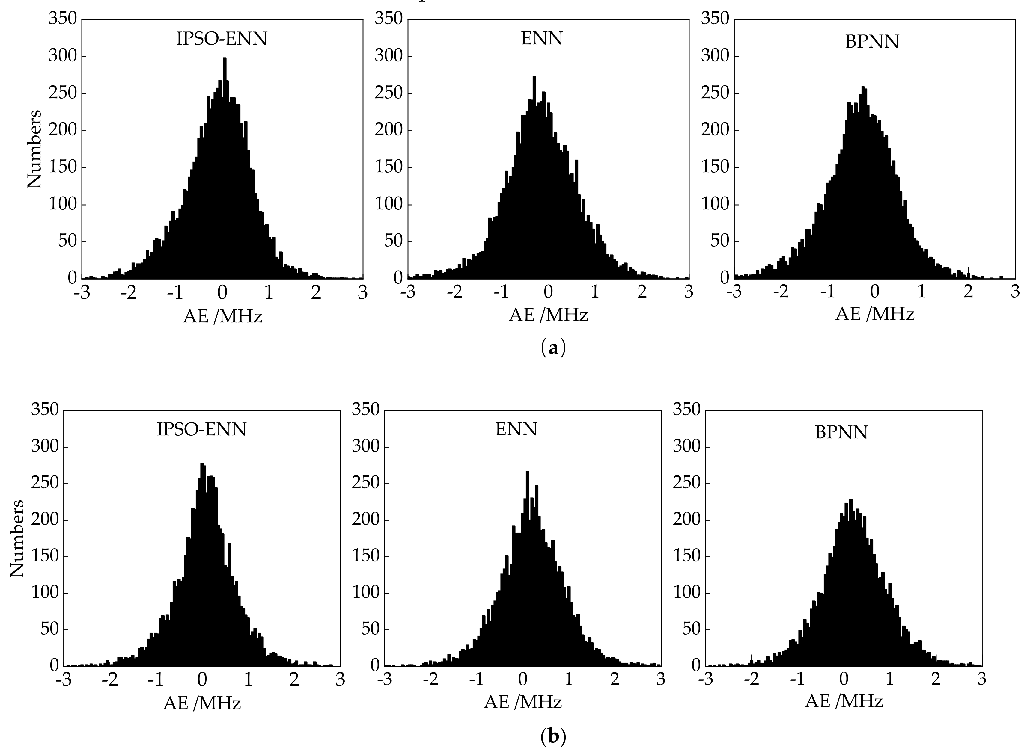
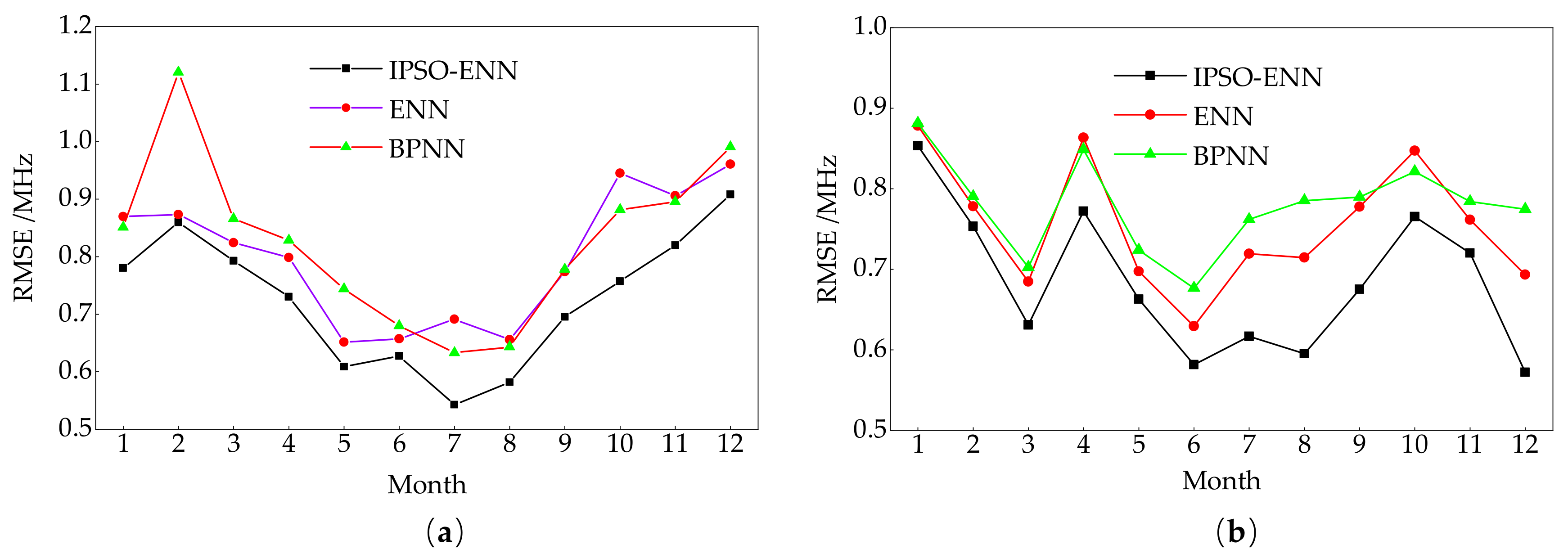
4. Discussion
5. Conclusions
Author Contributions
Funding
Acknowledgments
Conflicts of Interest
References
- Williscroft, L.A.; Poole, A. Neural Networks, foF2, sunspot number and magnetic activity. Geophys. Res. Lett. 1996, 23, 3659–3662. [Google Scholar] [CrossRef]
- Yue, X.N.; Wan, W.X.; Liu, L.B.; Ning, B.Q.; Zhao, B.Q. Applying artificial neural network to derive long-term foF2 trends in the Asia/Pacific sector from ionosonde observations. J. Geophys. Res. 2006, 111, 1–11. [Google Scholar] [CrossRef]
- Noraset, W.; Kornyanat, H.; Pornchai, S.; Takuya, T. A comparison of neural network-based predictions of foF2 with the IRI-2012 model at conjugate points in Southeast Asia. Adv. Space Res. 2017, 59, 2934–2950. [Google Scholar]
- Oyeyemi, E.O.; Poole, A.W.V.; McKinnell, L.A. On the global model for foF2 using neural networks. Radio Sci. 2005, 40, 1–15. [Google Scholar] [CrossRef]
- McKinnell, L.A.; Poole, A.W.V. Neural network-based ionospheric modelling over the South African region. S. Afr. J. Sci. 2004, 100, 519–523. [Google Scholar]
- Wang, R.P.; Zhou, C.; Deng, Z.X.; Ni, B.B.; Zhao, Z.Y. Predicting foF2 in the China region using neural networks improved by the genetic algorithm. J. Atmos. Sol. Terr. Phys. 2013, 92, 7–17. [Google Scholar] [CrossRef]
- Zhao, X.K.; Ning, B.Q.; Liu, L.B.; Song, G.B. A prediction model of short-term ionospheric foF2 based on AdaBoost. Adv. Space Res. 2014, 53, 387–394. [Google Scholar] [CrossRef]
- Li, P.X.; Wang, D.; Wang, L.J.; Lu, H.C. Deep visual tracking: Review and experimental comparison. Pattern Recognit. 2018, 76, 323–338. [Google Scholar] [CrossRef]
- Wen, L.L.; Zhou, K.L.; Yang, S.L.; Lu, X.H. Optimal load dispatch of community microgrid with deep learning based solar power and load forecasting. Energy 2019, 171, 1053–1065. [Google Scholar] [CrossRef]
- Acharya, R.; Roy, B.; Sivaraman, M.R.; Dasgupta, A. Prediction of ionospheric total electron content using adaptive neural network with in-situ learning algorithm. Adv. Space Res. 2011, 47, 115–123. [Google Scholar] [CrossRef]
- Jia, W.K.; Zhao, D.A.; Zheng, Y.J.; Hou, S.J. A novel optimized GA-Elman neural network algorithm. Orig. Artic. 2019, 31, 449–459. [Google Scholar] [CrossRef]
- Yun, P.P.; Ren, Y.F.; Xun, Y. Energy-Storage optimization strategy for reducing wind power fluctuation via Markov prediction and PSO method. Energies 2018, 11, 3393. [Google Scholar] [CrossRef]
- Fang, H.Q.; Shen, Z.Y. Optimal hydraulic turbogenerators pid governor tuning with an improved particle swarm optimization algorithm. Proc. CSEE 2005, 25, 120–124. [Google Scholar]
- Nakamura, M.I.; Maruyama, T.; Shidama, Y. Using a neural network to make operational forecasts of ionospheric variations and storms at Kokubunji. J. Natl. Inst. Inf. Commun. Technol. 2009, 56, 391–406. [Google Scholar] [CrossRef]
- Mandrikova, O.V.; Polozov, Y.A.; Soloviev, I.S.; Fetisova (Glushkova), N.V.; Zalyaev, T.L.; Kupriyanov, M.S.; Dmitriev, A.V. Method of analysis of geophysical data during increased solar activity. Pattern Recognit. Image Anal. 2016, 26, 406–418. [Google Scholar] [CrossRef]


| FACTOR | Diurnal and Seasonal Variation | Solar and Magnetic Activities | Present Value | ||||||
|---|---|---|---|---|---|---|---|---|---|
| VARIABLE | HRS | HRC | DNS | DNC | SSN | F10.7 | Kp | Dst | foF2 |
| YEAR | Annual Average | IPSO-ENN | ENN | BPNN | |||
|---|---|---|---|---|---|---|---|
| foF2/MHz | RMSE/MHz | RE/% | RMSE/MHz | RE/% | RMSE/MHz | RE/% | |
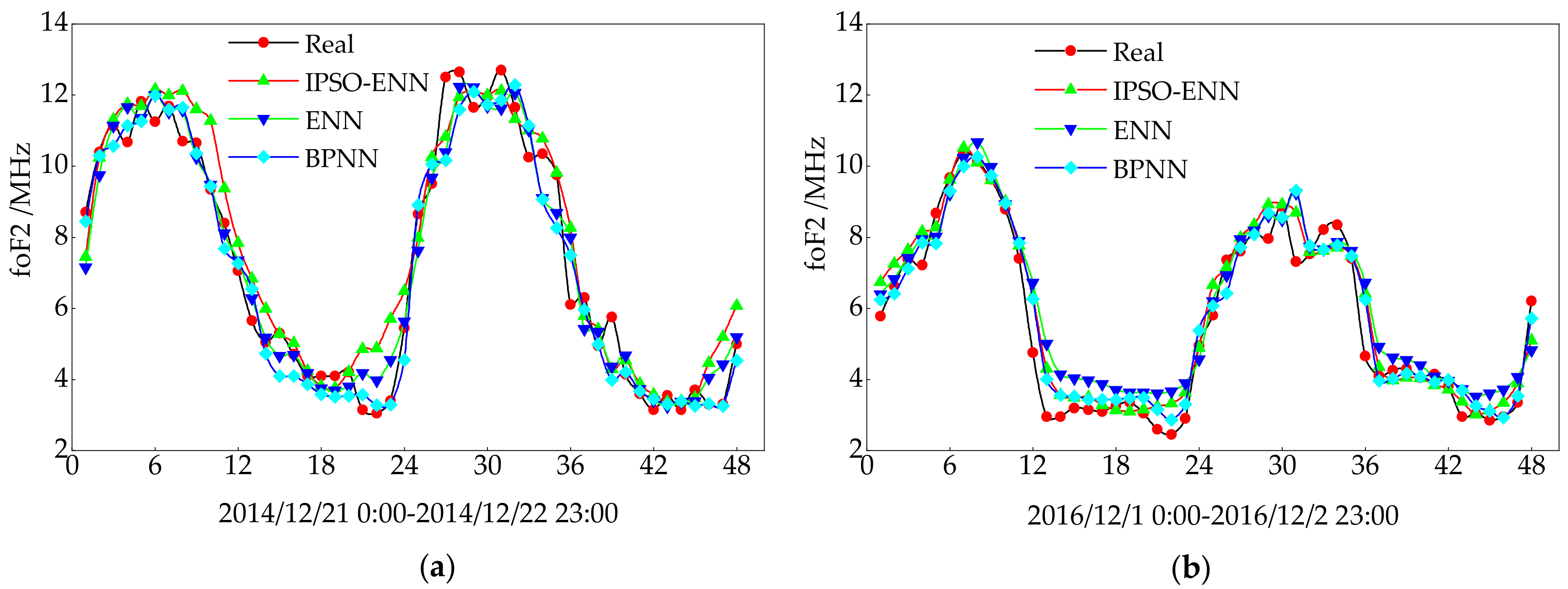
| 2014 | 8.19 | 0.75 | 7.58 | 0.81 | 8.53 | 0.85 | 8.66 |
| 2016 | 6.24 | 0.68 | 8.58 | 0.76 | 10.03 | 0.79 | 10.20 |
© 2019 by the authors. Licensee MDPI, Basel, Switzerland. This article is an open access article distributed under the terms and conditions of the Creative Commons Attribution (CC BY) license (http://creativecommons.org/licenses/by/4.0/).
Share and Cite
Fan, J.; Liu, C.; Lv, Y.; Han, J.; Wang, J. A Short-Term Forecast Model of foF2 Based on Elman Neural Network. Appl. Sci. 2019, 9, 2782. https://doi.org/10.3390/app9142782
Fan J, Liu C, Lv Y, Han J, Wang J. A Short-Term Forecast Model of foF2 Based on Elman Neural Network. Applied Sciences. 2019; 9(14):2782. https://doi.org/10.3390/app9142782
Chicago/Turabian StyleFan, Jieqing, Chao Liu, Yajing Lv, Jing Han, and Jian Wang. 2019. "A Short-Term Forecast Model of foF2 Based on Elman Neural Network" Applied Sciences 9, no. 14: 2782. https://doi.org/10.3390/app9142782
APA StyleFan, J., Liu, C., Lv, Y., Han, J., & Wang, J. (2019). A Short-Term Forecast Model of foF2 Based on Elman Neural Network. Applied Sciences, 9(14), 2782. https://doi.org/10.3390/app9142782