Multicriteria Prediction and Simulation of Winter Wheat Yield Using Extended Qualitative and Quantitative Data Based on Artificial Neural Networks

Abstract

Wheat is one of the main grain species as well as one of the most important crops, being the basic food ingredient of people and livestock. Due to the importance of wheat production scale, it is advisable to predict its yield before harvesting. However, the current models are built solely on the basis of quantitative data. Therefore, the aim of the work was to create three multicriteria models for the prediction and simulation of winter wheat yield, which were made on the basis of extended quantitative and qualitative variables from field research in the year period 2008–2015. Neural networks with MLP (multi-layer perceptron) topology were used to build the following models, which can predict and simulate the yield on three dates: 15 April, 31 May, and 30 June. For this reason, they were designated as follows: QQWW15_4, QQWW31_5, and QQWW30_6. Each model is based on a different number of independent features, which ranges from 19 to 25. As a result of the conducted analyses, a MAPE (mean absolute percentage error) forecast error from 6.63% to 6.92% was achieved. This is equivalent of an error ranging from 0.521 to 0.547 t·ha⁻¹, with an average yield of 6.57 ton per hectare of cultivated area. In addition, the most important quantitative and qualitative factors influencing the yield were also indicated. In the first predictive range (15 April), it is the average air temperature from 1 September to 31 December of the previous year (T9-12_PY). In the second predictive range (31 May) it is the sum of precipitation from 1 May to 31 May, and in the third (30 June) is the average air temperature from 1 January to 15 April of the year (T1-4_CY). In addition, one of the qualitative factors had a significant impact on the yield in the first phase-the type of forecrop in the previous year (TF_PY). The presented neural modeling method is a specific extension of the previously used predicting methods. An element of innovation of the presented concept of yield modeling is the possibility of performing a simulation before harvest, in the current agrotechnical season. The presented models can be used in large-area agriculture, especially in precision agriculture as an important element of decision-making support systems.

1. Introduction

For many years, scientists from all over the world have been creating and are still improving plant yield models [1]. Yield simulation models based on growth processes have become more and more evident in the last decades mainly in studies on the impact of climate on agricultural production. Their usefulness is significant in understanding the relationship between genotype, environment and management to aid decision-making in farms, including cultivars selection, sustainable farm management, and economic planning [2]. Yield models are imperfect approximations to the real interactions between biotic and abiotic factors, designed mainly as tools that provide useful information to farmers, researchers, and policy-makers [3]. Predictive models allow users to simulate a potential yield depending on agrotechnical and weather conditions. This is an important element of precision farming, which allows simulation of the expected yield before harvest, and consequently to optimize the entire production process [4]. Therefore, plant yield models are applied in order to create prognostic tools that can be an important element of decision support systems [5]. Projecting the quantity and quality of yields of various cultivars of plants is very important as it affects the planning of the entire production process, including: Application of proper production means, decision-making, transport, storage, and risk management [6,7]. The ability of the simulation model to capture the historical variability of cereal yields has shown that it can serve as a basis for indicating the usefulness of yield models among interested parties [2]. Plant production is strongly determined by the course of weather conditions during vegetation, which can often be intense and lead to strong fluctuations, caused by continuous climate change in the world. Climate change is a threat to increasing food production in some regions [8]. Therefore, the integration of meteorological data and cultivation data is an important element in the produced models [9,10].

There are many methods of analyzing yield components that can be used to implement the task. Techniques such as analysis of variance, Pearson correlation coefficient, multiple regression, and path analysis are usually used to analyze yield components [11]. The main problem of regression models is that they are unable to explain the non-linear and complex relationship between the yield and their components [12]. To overcome this problem, in recent years, agricultural scientists have used artificial intelligence (AI) tools, such as artificial neural networks (ANN), genetic expression programming (GEP), and the adaptive neuro-fuzzy interference system (ANFIS) [10,13,14,15,16,17]. One of the most common types of ANNs that are used in biological research is the multi-layer perceptron (MLP) [12,18,19,20]. MLP is an ANN model of the feed-forward type, which consists of the input layer, the hidden layer and the output layer. The MLP has many layers connected to each other, and each node is a neuron with a non-linear activation function. Perceptron calculates a single result from multiple inputs, creating a linear combination according to its inputs, and then determines the result using the non-linear transfer function [21]. Plant yield prediction methods based on combining images using remote sensing methods are also gaining popularity. The normalized differential vegetation index (NDVI) is the most commonly used in this type of analysis [22,23,24]. However, many researchers use a unifying theory, the Golden Rule of forecasting—a conservative theory. A cautious prediction is consistent with the combined knowledge of both present and the past. To be conservative, the forecasters must search and use all knowledge relevant to the problem, including knowledge about the methods used for the given situation [25].

Models created for the prediction of crop yields are most often based on numerical data. This approach is most often generalized because it allows the use of many different methods of linear and nonlinear modeling. However, there are cases in which this approach is insufficient, then the following qualitative or quantitative-qualitative data are applied. Many researchers show that combining different types of predictions leads to the better results than using only one method [26,27]. Combining the prediction model is also the subject of literature using various innovative hybrid methods that show the superiority of combining yield forecasts in relation to particular methods [28].

Similar models are presented in the paper [10], but they concern the forecasting of yield of another species, i.e., winter rape. The same forecast dates were proposed in this paper, but the forecasting models were based solely on quantitative data. Other works with models: Quantitative data: Measurement of NDVI and SAVI (Soil-adjusted vegetation index) vegetation indices. Al-Gaadi et al. [29] applied the linear regression method to create a mathematical description of potato yielding and to show the relationship between actual and predicted yields based on remote sensing measurements. In the work Al-Hamed and Wahba [30] artificial neural networks were used to forecast potato yields on the basis of energy inputs incurred in Saudi Arabia. Input variables: Human labor energy, machine energy, diesel oil, fertilizers, pesticides, seeds, and irrigation were typically quantitative variables. Potato yield was assumed to be a dependent variable. All values were calculated per one hectare of crop and transformed into energy forms enabling the analysis. There are no studies in which both quantitative and qualitative data are used to construct predictive models. This is mainly due to the fact that most of the models are based on classical methods, which significantly limit the full use of linguistic (qualitative) variables.

Wheat is one of the main grain species as well as one of the most important cultivated crops is the basic food product of people and livestock. It is grown mainly in Europe, Canada, Russia, and the United States. Global cereal production in 2017 amounted to 2,980,174,798 tons, with the share of wheat production 771,718,579 tons, which is more than 25% of the global cereal production. In the European Union, cereal production in 2017 was 307,061,987 tons, with the share of wheat production 150,224,838 tons, which accounts for almost 49% of EU production. In contrast, the volume of Polish wheat production amounted to 11,665,702 tons and accounts for almost 8% of EU production with an average yield of 48.7 dt per hectare of growing area. The total wheat cultivation area in Poland in 2017 was 2,391,853 ha [31].

Bearing in mind the above, the authors of the following work have undertaken a task to develop new multi-criteria (on the basis of prediction date), hybrid (on the basis of data type) winter wheat yield models that will use quantitative and qualitative data by means of artificial neural networks. The purpose of this work is to build three independent models built on the basic data obtained from each farm, i.e., on weather and agrotechnical information. It is assumed that each model will be based on 19 basic independent features, while subsequent models will be created based on additional data from subsequent prediction dates, i.e., 15 April, 31 May, and 30 June. All data was obtained from cultivated fields of winter wheat and mobile meteorological stations. It has been assumed that the generated models will have a MAPE (mean absolute percentage error) value below 7%.

2. Materials and Methods

Creating multicriteria prediction neural models was performed by collecting data in the period 2008–2015 of winter wheat from cultivation area located in Poland, in the central and south-western part of Greater Poland, with emphasis on districts of Poznań (52°24′29.759″ N 16°56′0.672″ E), Kościan (52°5′10.77″ N 16°38′41.998″ E), and Gostyń (51°53′5.762″ N 17°0′47.829″ E; Figure 1). For the construction and verification of model, data from 301 fields were collected (

Table 1. The number of arable fields of winter wheat divided into two sets, A and B.

	Set A							Set B
Year	2008	2009	2010	2011	2012	2013	2014	2015
Number of fields	37	34	36	51	15	30	52	46

). The following information constituted a database for the creation of predictive neural models with two sets, A and B. Set A (255 fields) makes up the data for model building from 2008–2014, whereas set B (45 fields) includes only 2015, which was not used in the model, but was used for model validation.

Meteorological data for the research area, such as air temperature, precipitation, and period, were collected from Davis stationary and mobile meteorological stations close to the research area—Kórnik, Gola, Turew, Piotrowo, and Stary Gołębin.

Neural predictive models took into account three dates in a calendar year: 15 April, 31 May, and 30 June. The models were named in the following way: QQWW15_4 (QuantitativeQualitativeWinterWheat15_April), QQWW31_5, and QQWW30_6. The independent variables that influence crop yields could be easily accessed by agricultural producers (

Table 2. Data structure in neural prediction models.

Symbol	Unit of Measure	Variable Name	Model QQWW15_4	Model QQWW31_5	Model QQWW30_6	The Scope of Data
Quantitative Data
R9-12_PY	mm	The sum of precipitation from 1 September to 31 December of the previous year	+	+	+	63–234
T9-12_PY	°C	The average air temperature from 1 September to 31 December of the previous year	+	+	+	4.9–9.4
R1-4_CY	mm	The sum of precipitation from 1 January to 15 April of the current year	+	+	+	59–185
T1-4_CY	°C	The average air temperature from 1 January to 15 April of the current year	+	+	+	−0.4–4.9
R4_CY	mm	The sum of precipitation from 1 April to 30 April of the current year	−	+	+	8.7–60.4
T4_CY	°C	The average air temperature from 1 April to 30 April of the current year	−	+	+	5.9–12.2
R5_CY	mm	The sum of precipitation from 1 May to 31 May of the current year	−	+	+	14.2–132.5
T5_CY	°C	The average air temperature from 1 May to 31 May of the current year	−	+	+	11.8–16.2
R6_CY	mm	Total precipitation from 1 June to 30 June of the current year	−	−	+	15–121
T6_CY	°C	The average air temperature from 1 June to 30 June of the current year	−	−	+	14.2–19.6
N_LY	kg ha−1	The sum of N fertilization-autumn in the previous year	+	+	+	0–100
N_CY	kg ha−1	The sum of N fertilization-spring in the current year	+	+	+	68–359
P2O5_CY	kg ha−1	The sum of P2O5 fertilization in the current year	+	+	+	0–82
K2O_CY	kg ha−1	The sum of K2O fertilization in the current year	+	+	+	0–151
MGO_CY	kg ha−1	The sum of MgO fertilization in the current year	+	+	+	0–46
SO3_CY	kg ha−1	The sum of SO3 fertilization in the current year	+	+	+	14–115
CU_CY	g ha−1	The sum of Cu fertilization in the current year	+	+	+	10–138
MN_CY	g ha−1	The sum of Mn fertilization in the current year	+	+	+	40–360
ZN_CY	g ha−1	The sum of Zn fertilization in the current year	+	+	+	9–226
DOF_PY	t ha−1	The dose of organic fertilizer in the previous year	+	+	+	0–36
Qualitative Data
KOF_PY	word	The kind of organic fertilizer in the previous year	+	+	+	No, Livestock manure, Chicken manure.
LF_PY	word	The field liming in the previous year	+	+	+	Yes, No.
ST_PY	word	The soil tillage in the previous year	+	+	+	Aggregate cultivator, Shallow tillage, Deep tillage, Ploughing.
KSD_PY	word	The kind of sowing date in the previous year	+	+	+	Early, Optimal, Tardy.
TF_PY	word	The type of forecrop in the previous year	+	+	+	Winter rapeseed, Winter wheat, Winter triticale, Winter barley, Spring barley, Sugar beet, Potatoes, Alfalfa, Sunflower, Mustard, Maize.

“+”—the variable exists in the model, “−”—the variable does not exist in the model.

).

The following model of winter wheat yield prediction makes it possible to forecast and simulate expected yields directly before harvesting, in the current agricultural year.

The data collected to build and verify the correctness of the models were the basis for the development of software, commissioned by farms located in Poland (Greater Poland), using fields covered by their own research. Specific prediction dates used in the models, i.e., 15.04, 31.05, and 30.06, were proposed by agronomists working in the area. The use of unambiguous calendar year dates is more practical from the point of view of agricultural production. The proposed prediction dates make it much easier to monitor winter wheat yielding. Moreover, they are selected in such a way as to reflect as much as possible the key stages of vegetation in typical years, i.e., 15.04—the shooting phase, 31.05—the earing phase, and 30.06—the beginning of full maturity.

2.1. Method of Constructing Neural Models

For the creation of neural models, the independent variables were chosen so that each neural network used a different number of independent variables from Table 1 and Table 2.

For the selection of network topology and learning method, network’s ability to approximate and generalize was accounted for, basing on network quality measures. By using the Statistica v7.1 (StatSoft Inc., Tulsa, OK, USA) the testing of networks with different architectures was carried out. With an automatic network designer (AND) each of the models QQWW15_4, QQWW31_5, and QQWW30_6 tested 20,000 networks per each. Network selection was performed based on the best parameters of network quality determination.

The set of empirical data was divided randomly into a learning set, a validation set, and a test set. The sets’ sizes included the learning set—211 cases; validation set—45 cases; and testing set—45 cases. The proportion of sets was 70%, 15%, 15% that considered the number of studied fields.

2.2. Methodology for Validating the Neural Models

With the use of the automatic network designer, each model was evaluated by considering data from Statistica (StatSoft Inc., Tulsa, OK, USA) software, namely the standard deviation, mean error, error deviation, mean absolute error, deviation quotient, and correlation. By considering the smallest value of the mean absolute error and the largest value of the correlation, the best model was chosen.

By comparing data from set B with the predictions from set A, the predictive ability of the constructed neural models was assessed using ex post measures of the prediction error.

The following errors were calculated on the basis of past data, namely predictions that were out-of-date and the corresponding current values of the predicted variable. In such a case, the prediction error is the difference between the observed and predicted value.

Validation of the constructed models was carried out by investigating last year’s data of the study (2015) as well as 46 fields of winter wheat. However, the following data was not taken into consideration in the construction of the neural models. The evolution of the prediction quality was done by using the available methodology in the literature [10,12,32,33,34,35].

• RAE—relative approximation error;

  $$RAE =\sqrt{\frac{{{\displaystyle \sum }}_{i =1}^n{\left(y_i-{\widehat{y}}_i\right)}^2}{{{\displaystyle \sum }}_{i =1}^{n }{\left(y_i\right)}^2}}.$$

  (1)
• RMS—root mean square error;

  $$RMS =\sqrt{\frac{{{\displaystyle \sum }}_{i =1}^{n }{\left(y_i-{\widehat{y}}_i\right)}^2}{n}}.$$

  (2)
• MAE—mean absolute error;

  $$MAE =\frac{1}{n}{{\displaystyle \sum }}_{i =1}^n\left|y_i-{\widehat{y}}_i\right|.$$

  (3)
• MAPE—mean absolute percentage error;

  $$MAPE =\frac{1}{n}{{\displaystyle \sum }}_{i =1}^n\left|\frac{y_i-{\widehat{y}}_i}{y_i}\right|\times 100\%,$$

  (4)

where,

• n—number of observations,
• $y_i$—actual values obtained during research,
• ${\widehat{y}}_i$—values given by the model.

For better visualization of dependency between observed and predicted yield, graphs were created showing relations for each prediction date.

2.3. Neural Network Sensitivity Analysis

The sensitivity of neural networks under construction was carried out in order to check which of the examined independent features was the most beneficial variable for winter wheat biological yields. By removing a specific input variable (independent trait) from the model the influence on the neural network total error can be observed, which allows to determine the significance (on the output variable, i.e., yield) of individual independent features. For this purpose, two indicators were used. Error quotient—the ratio of error to error obtained by all independent features—the larger this value, the greater is the importance of the given trait. If it is less than 1, it might be removed from the model in order to improve its quality, although this is not obligatory. Rank shows in numerical terms the ordering of the features by decreasing error, a rank of 1 indicates the network’s greatest importance.

3. Results

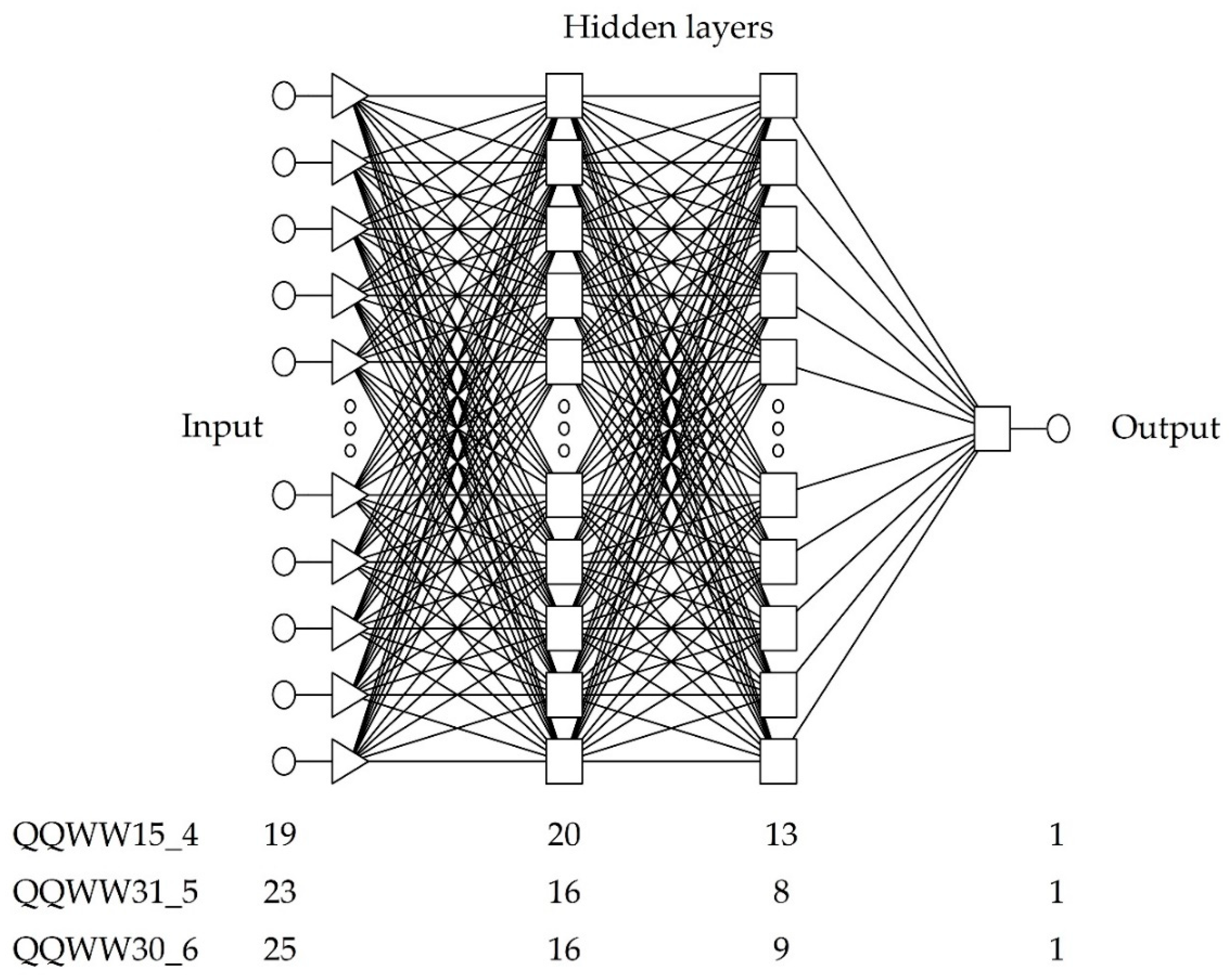
As a result of the analyses, each neural model was chosen for each prediction date. Basic information on the quality of QQWW15_4, QQWW31_5, and QQWW30_6 is given in

Table 3. The quality and structure of the neural models produced.

	QQWW15_4	QQWW31_5	QQWW30_6
Neural network structure	MLP 19:35-20-13-1:1	MLP 23:38-16-8-1:1	MLP 25:39-16-9-1:1
Learning error	0.0579	0.0721	0.0781
Validation error	0.0707	0.0564	0.0664
Test error	0.1517	0.0835	0.0996
Mean	6.5785	6.5785	6.5785
Standard deviation	1.5707	1.5707	1.5707
Average error	0.0164	0.0285	−0.0029
Deviation error	0.7188	0.8624	0.8952
Mean Absolute error	0.5041	0.6635	0.6802
Quotient deviations	0.4576	0.5491	0.5722
Correlation	0.8896	0.8386	0.8201

. The general structure of the designed neural network model is presented in Figure 2.

To determine the quality of prediction, computations applied for ex post methods were performed, using the Formulae (1)–(4). The results are given in

Table 4. Measures prediction ex post of analyzed neural models.

Model	RAE (−)	RMS (t ha−1)	MAE (t ha−1)	MAPE (%)
QQWW15_4	0.069	0.567	0.542	6.92
QQWW31_5	0.066	0.618	0.521	6.63
QQWW30_6	0.068	0.619	0.547	6.88

.

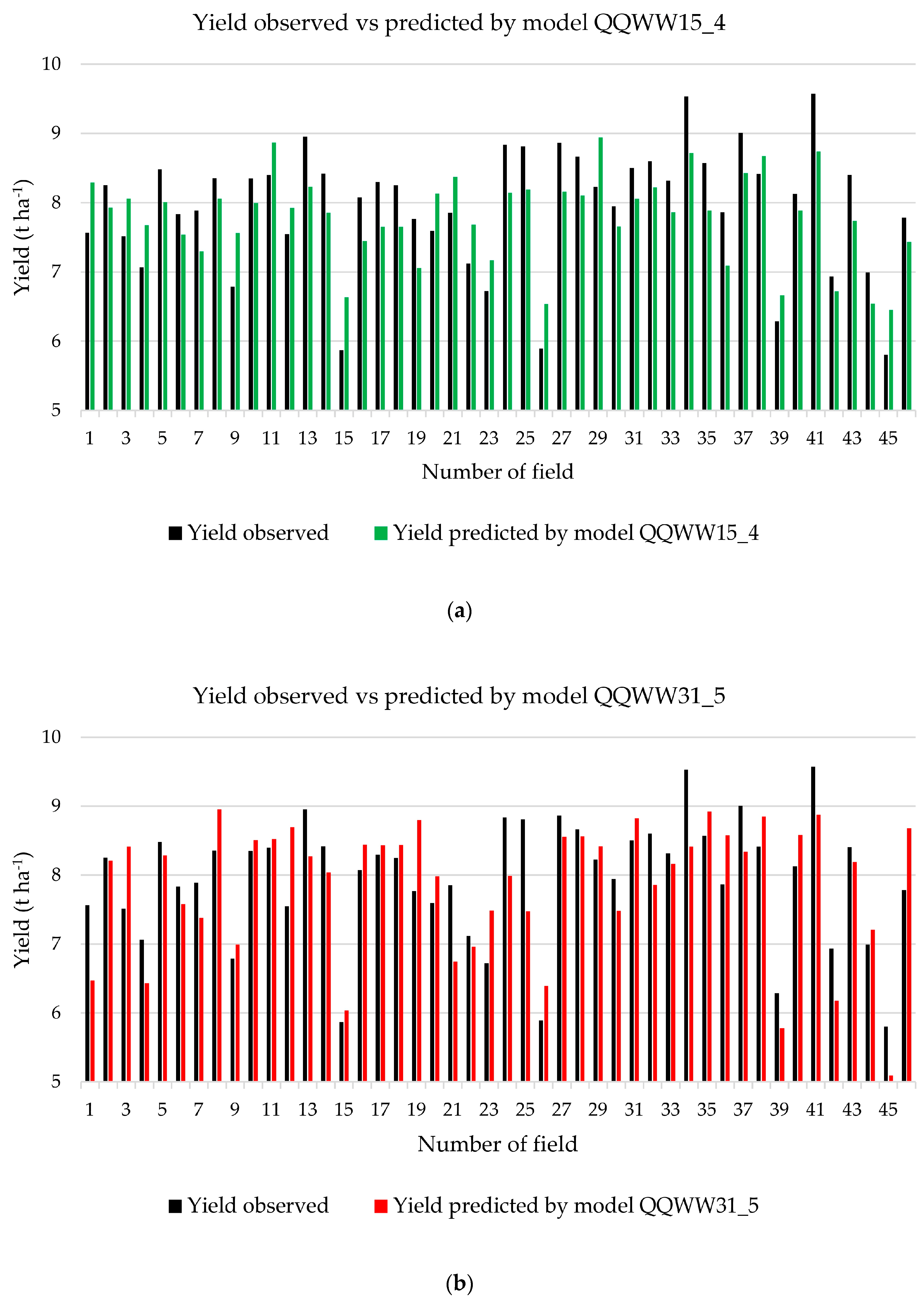
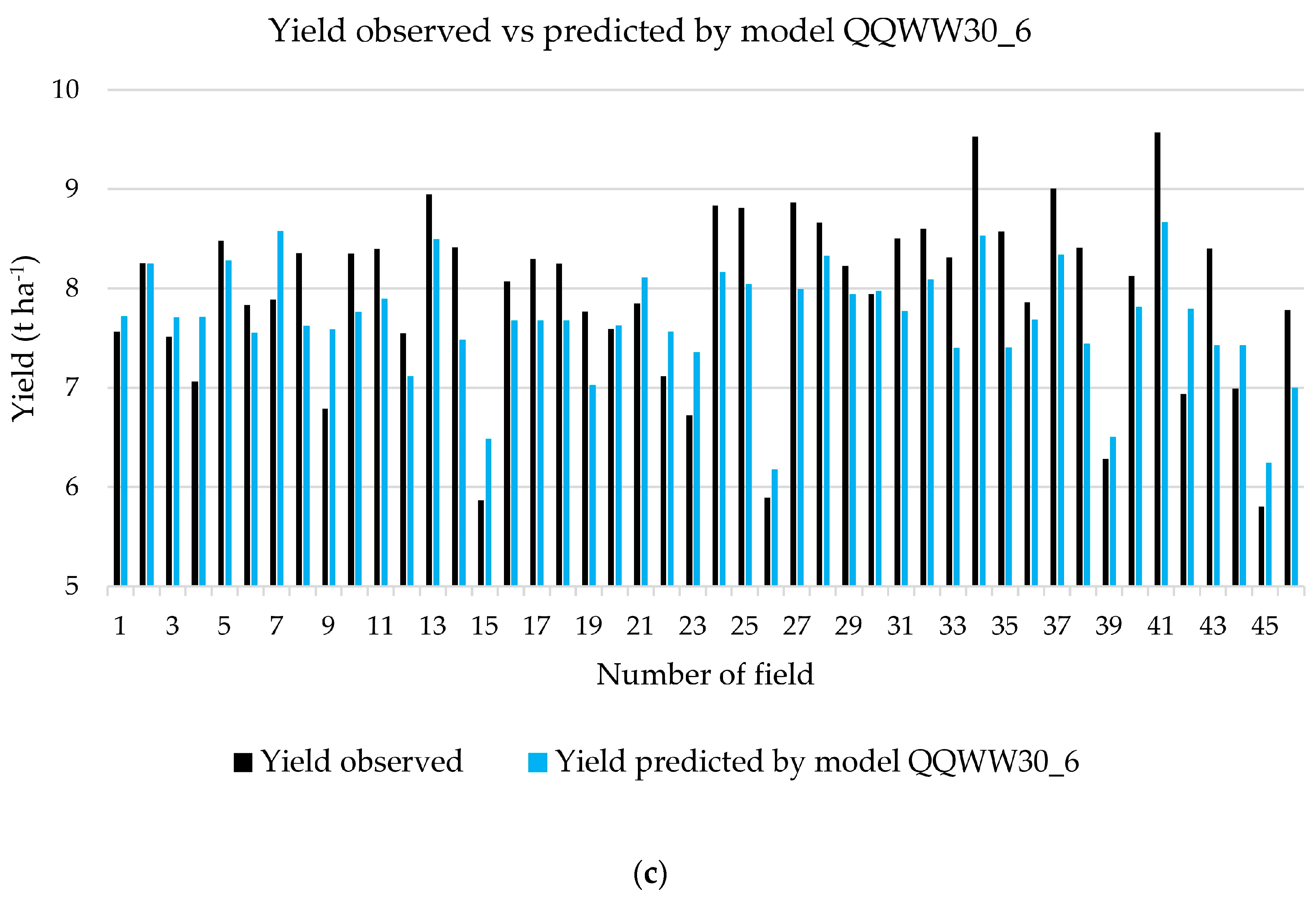
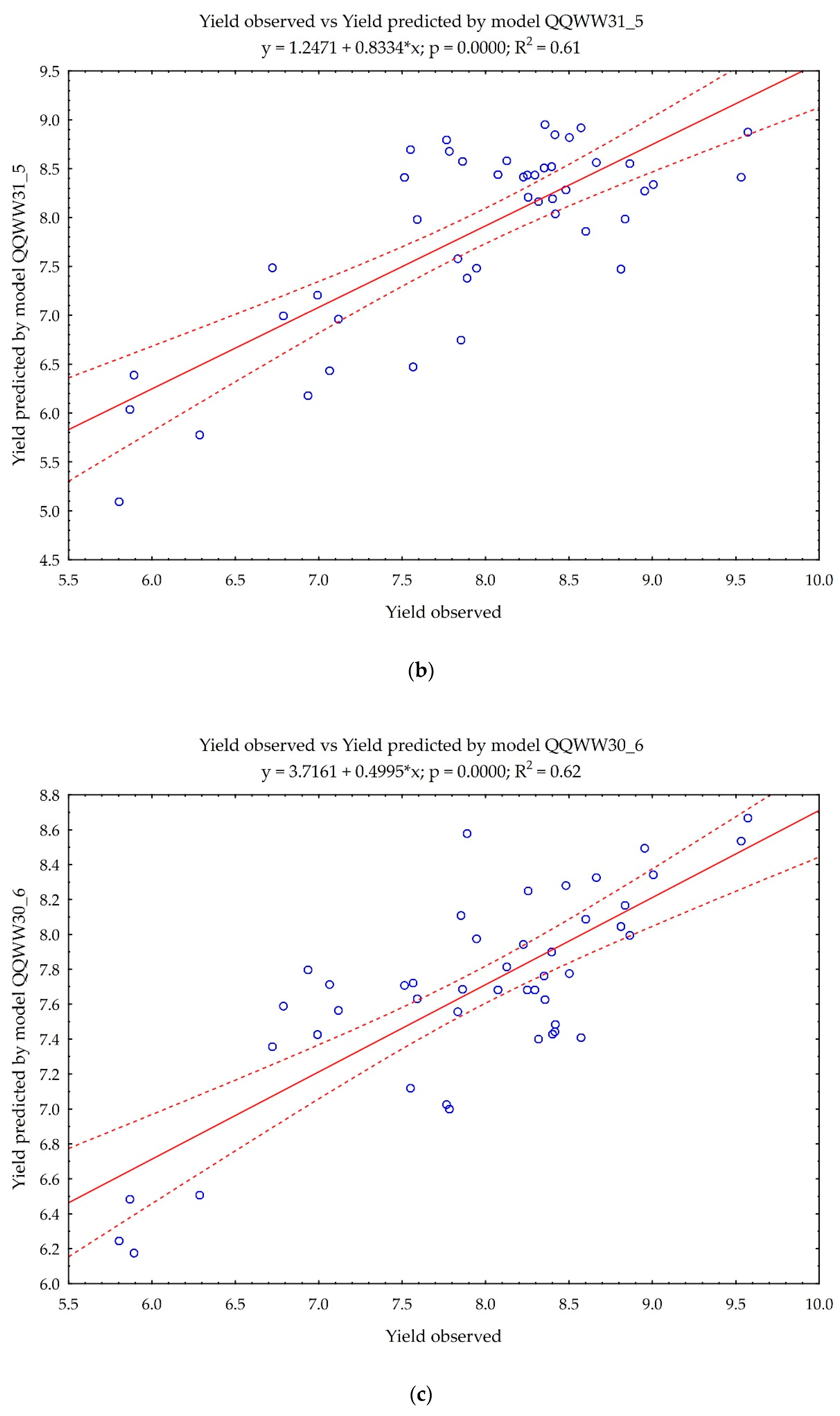
In the next step, graphs were plotted showing the relationship between the actual and predicted yield for each date. Figure 3 presents relationship for QQWW15_4, QQWW31_5, and QQWW30_6 respectively.

Network Sensitivity Analysis

In the last step of the calculations, network sensitivity analysis was carried out for all constructed neural models. The results of this analysis are shown in

Table 5. Sensitivity analysis of neural networks.

Variable	Model
	QQWW15_4		QQWW31_5		QQWW30_6
	Quotient	Rank	Quotient	Rank	Quotient	Rank
R9-12_PY	1.1381	9	1.0114	13	1.0155	19
T9-12_PY	1.3673	1	1.0420	7	1.1622	2
R1-4_CY	1.2296	4	1.0070	18	1.1580	3
T1-4_CY	1.0476	13	1.0091	15	1.1720	1
R4_CY	−	−	1.0091	16	1.0049	23
T4_CY	−	−	1.0241	10	1.1572	4
R5_CY	−	−	1.1576	1	1.0986	6
T5_CY	−	−	1.1333	2	1.0670	8
R6_CY	−	−	−	−	1.0081	22
T6_CY	−	−	−	−	1.0604	10
N_LY	1.0174	19	1.0029	20	1.0027	24
N_CY	1.0417	16	1.0060	19	1.0021	25
P2O5_CY	1.0441	15	1.0847	5	1.0290	13
K2O_CY	1.1039	12	0.9975	22	1.0101	21
MGO_CY	1.1078	11	1.0109	14	1.0623	9
SO3_CY	1.0451	14	1.0289	9	1.0132	20
CU_CY	1.0307	17	1.0170	12	1.0163	17
MN_CY	1.1809	6	0.9943	23	1.0549	11
ZN_CY	1.1125	10	1.0084	17	1.1103	5
DOF_PY	1.0233	18	0.9976	21	1.0275	14
KOF_PY	1.1783	7	1.0331	8	1.0245	16
LF_PY	1.2359	3	1.0205	11	1.0268	15
ST_PY	1.2250	5	1.1155	3	1.0156	18
KSD_PY	1.1403	8	1.0588	6	1.0521	12
TF_PY	1.2590	2	1.1094	4	1.0787	7

.

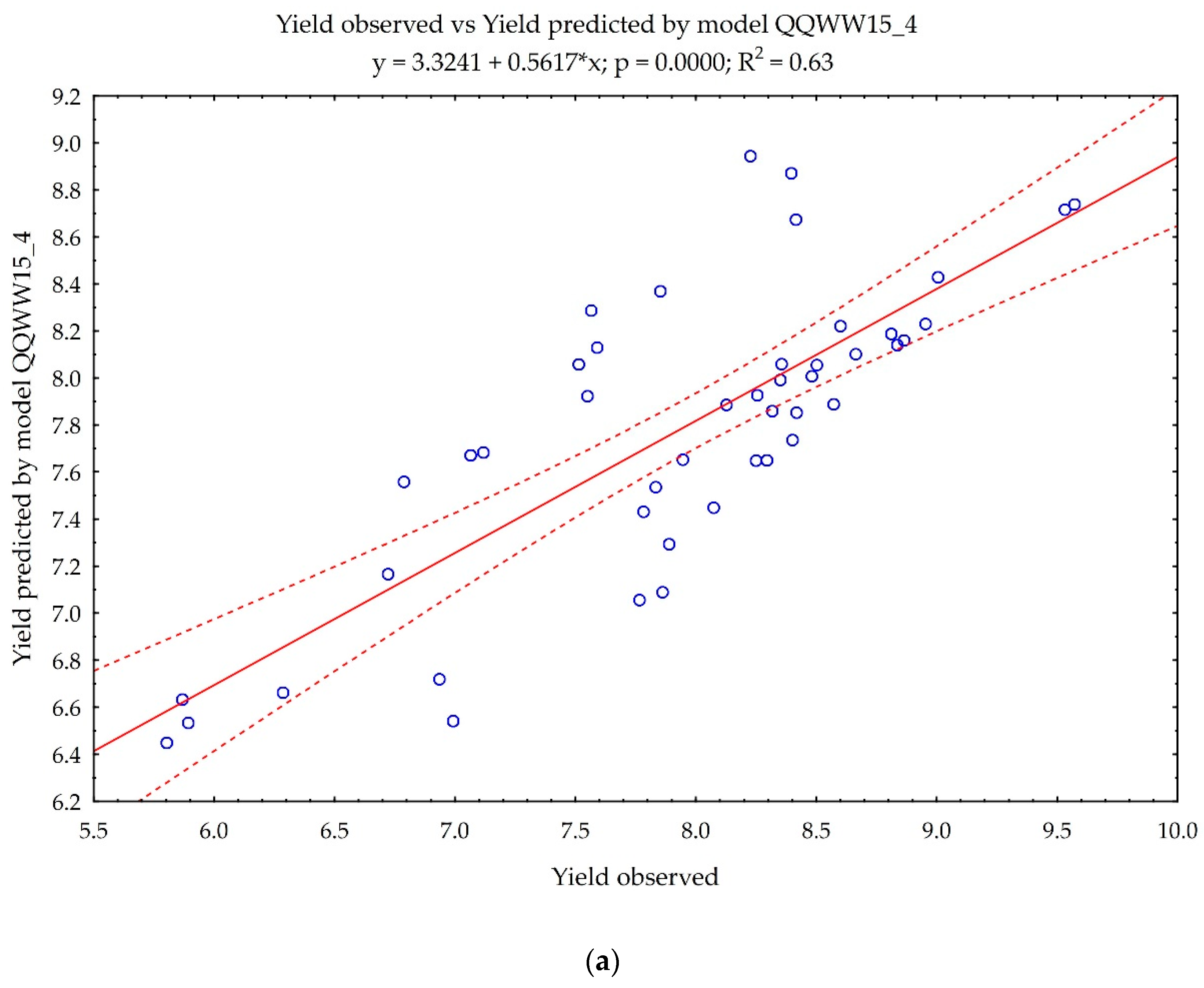
As Figure 4 shows, the best match between the observed yield and the predicted yield can be found in model QQWW15_4, for which the determination coefficient R² was 0.63. The other models slightly vary. In model QQWW31_5, the determination coefficient, R², of 0.61 was obtained, while in model QQWW30_6, the coefficient, R² was 0.62.

4. Discussion

Plant yield prediction is based on historical empirical data, which most often appear in the form of quantitative data, such as anthropogenic, climatic, and geomorphological factors. Such a large number of variables necessary to generate a properly functioning prognostic model causes problems with choosing an appropriate modeling method. In addition, some data can be obtained only from specific researches [36], however it can only be used for scientific purposes. Therefore, in the following work, the authors created three predictive neural models that give the possibility of their use in the current agrotechnical season before harvesting. These models are based on data available for each farmer and are based on two types of data: Quantitative and qualitative. This is a new approach to problems in the prediction of crop yields. The assumption was made that MAPE for each generated predictive model would be lower than 7%. It was assumed that the correct functioning of the created neural models will be verified by comparing the obtained predicted with the observed wheat yields in the last (2015) year of the study.

The neural modeling method used for performance of nonlinear tasks gives better results compared to classic statistical methods [11,37]. A common problem in the neural network of plant yield prediction is the selection of the appropriate network topology. From the literature sources [10,33], the MLP network, also known as multilayer perceptron, is most commonly used in terms of forecasting. In this work, three models based on the above type of network were created: QQWW15_4, QQWW31_5, and QQWW30_6. Each of the models was based on quantitative and qualitative data, which were 19, 23, and 25 independent variables respectively, with each model having five qualitative variables (Table 2).

Four ex post error measures were used in the work, i.e., relative approximation error (RAE), root mean square error (RMS), mean absolute error (MAE), and mean absolute percentage error (MAPE). They were used to determine the quality of models and to determine the errors of winter wheat yield prediction. Table 4 presents the error values of the ex post measures for all created neural models. The most commonly used indicators characterizing prediction error values include MAPE [10,34,38,39,40,41,42]. The lowest MAPE values were obtained for the QQWW31_5 neural model based on the MLP network of the 23:38-16-8-1:1 structure, which was 6.63%. Bearing in mind the critical level of MAPE at a complex level of up to 7%, the results obtained for all models were highly satisfactory, as they ranged up to 6.92% (for the QQWW15_4 model).

After all the calculations were completed, a network sensitivity analysis was performed for all the generated neural models. The meteorological data (Table 5) obtained the highest rank 1 for all networks. The result was similar to those obtained in earlier studies [35]. The following shows that the weather factors T9-12_PY, T1-4_CY, and R5_CY had the greatest impact on the winter wheat yield. The occurrence of optimal temperatures in the autumn season decided on the proper pullulation and preparation of plants to inhibit vegetation. However, appropriate thermal conditions that prevail during winter guarantee proper overwintering and good preparation of plants into spring vegetation. The appearance of any temperature anomalies during these periods may lead to a reduction in yield [43]. Another significant factor was the sum of rainfall from 1 May to 31 May the actual year. This period was a phase of critical water demand for winter wheat—from the beginning of shooting to the beginning of earing [44]. Water shortage results in a poor increase of assimilation organs and poor ear formation. Maintaining optimal thermal conditions during this period leads to the proper formation of subsequent development phases by plants and good grain yield. In the model QQWW31_5 and QQWW30_6, rank 2 was obtained by T9-12_PY and T5_CY. An interesting fact is that the QQWW15_4 model determined the TF_PY feature in the second position—the type of forecrop in the previous year. It follows that the applied technology and level of fertilization was properly adapted to the nutritional needs of winter wheat and was based on the real level of micro and macro elements in the soil. Only the QQWW15_4 model showed the second feature in the second position, which might mean that the left remains of forecrop in soil had a positive influence on the initial winter wheat growth process. Their beneficial effect was related by the inhibition of weed germination and the development of soil microorganisms, enriching the soil with nutrients, and scarifying the arable layer [45].

When comparing the values of the predicted yield to the observed yield (Figure 4), a similar match to each model was found—the R² was 0.61–0.63 making it acceptable.

5. Conclusions

The results of analyses presented in the work showed that multicriteria prediction neural models based on quantitative and qualitative data were a good tool for making forecasts and simulations of winter wheat crop before harvesting. Obtained results of MAPE, which did not exceed 7%, should be considered as very good. Most of the results obtained in the work, which were based on the analysis of network sensitivity, were consistent with the results of other authors’ works, indicating the dominant influence of the course of meteorological conditions on the yield of plants—winter wheat as well. The presented models can be used in precision agriculture as an element of decision support systems.

Further research should be carried out to optimize models in three directions. First—focusing on the reduction of independent features while maintaining low MAPE level. Second—obtaining data from more fields and from areas with different soil and climatic conditions. Third—performing a detail research of how the yield of winter wheat changes in different meteorological conditions prevailing during the growing season.

References

1. Salo, T.J.; Palosuo, T.; Kersebaum, K.C.; Nendel, C.; Angulo, C.; Ewert, F.; Bindi, M.; Calanca, P.; Klein, T.; Moriondo, M.; et al. Comparing the performance of 11 crop simulation models in predicting yield response to nitrogen fertilization. J. Agric. Sci. 2016, 154, 1218–1240. [Google Scholar] [CrossRef]
2. Ruane, A.C.; Hudson, N.I.; Asseng, S.; Camarrano, D.; Ewert, F.; Martre, P.; Boote, K.J.; Thorburn, P.J.; Aggarwal, P.K.; Angulo, C.; et al. Multi-wheat-model ensemble responses to interannual climate variability. Environ. Model. Softw. 2016, 81, 86–101. [Google Scholar] [CrossRef] [Green Version]
3. Ramirez-Villegas, J.; Koehler, A.K.; Challinor, A.J. Assessing uncertainty and complexity in regional-scale crop model simulations. Eur. J. Agron. 2017, 88, 84–95. [Google Scholar] [CrossRef] [Green Version]
4. Gonzalez-Sanchez, A.; Frausto-Solis, J.; Ojeda-Bustamante, W. Predictive ability of machine learning methods for massive crop yield prediction. Span. J. Agric. Res. 2014, 12, 313–328. [Google Scholar] [CrossRef]
5. Park, S.J.; Hwang, C.S.; Vlek, P.L.G. Comparison of adaptive techniques to predict crop yield response under varying soil and land management conditions. Agric. Syst. 2005, 85, 59–81. [Google Scholar] [CrossRef]
6. Gonzalez-Sanchez, A.; Frausto-Solis, J.; Ojeda-Bustamante, W. Attribute selection impact on linear and nonlinear regression models for crop yield prediction. Sci. World J. 2014, 2014, 509429. [Google Scholar] [CrossRef]
7. Kantanantha, N.; Serban, N.; Griffin, P. Yield and price forecasting for stochastic crop decision planning. J. Agric. Biol. Environ. Stat. 2010, 15, 362–380. [Google Scholar] [CrossRef]
8. Cordeiro, M.; Rotz, A.; Kroebel, R.; Beauchemin, K.; Hunt, D.; Bittman, S.; Koenig, K.; McKenzie, D. Prospects of Forage Production in Northern Regions under Climate and Land-Use Changes: A Case-Study of a Dairy Farm in Newfoundland, Canada. Agronomy 2019, 9, 31. [Google Scholar] [CrossRef]
9. Nelson, G.C.; Valin, H.; Sands, R.D.; Havlík, P.; Ahammad, H.; Deryng, D.; Elliott, J.; Fujimori, S.; Hasegawa, T.; Heyhoe, E.; et al. Climate change effects on agriculture: Economic responses to biophysical shocks. Proc. Natl. Acad. Sci. USA 2014, 111, 3274–3279. [Google Scholar] [CrossRef]
10. Niedbała, G. Application of artificial neural networks for multi-criteria yield prediction of winter rapeseed. Sustainability 2019, 11, 533. [Google Scholar] [CrossRef]
11. Niazian, M.; Sadat-Noori, S.A.; Abdipour, M. Modeling the seed yield of Ajowan (Trachyspermum ammi L.) using artificial neural network and multiple linear regression models. Ind. Crops Prod. 2018, 117, 224–234. [Google Scholar] [CrossRef]
12. Emamgholizadeh, S.; Parsaeian, M.; Baradaran, M. Seed yield prediction of sesame using artificial neural network. Eur. J. Agron. 2015, 68, 89–96. [Google Scholar] [CrossRef]
13. Niedbała, G. Simple model based on artificial neural network for early prediction and simulation winter rapeseed yield. J. Integr. Agric. 2019, 18, 54–61. [Google Scholar] [CrossRef] [Green Version]
14. Wojciechowski, T.; Niedbala, G.; Czechlowski, M.; Nawrocka, J.R.; Piechnik, L.; Niemann, J. Rapeseed seeds quality classification with usage of VIS-NIR fiber optic probe and artificial neural networks. In Proceedings of the 2016 International Conference on Optoelectronics and Image Processing (ICOIP 2016), Warsaw, Poland, 10–12 June 2016; pp. 44–48. [Google Scholar]
15. Niedbała, G.; Mioduszewska, N.; Mueller, W.; Boniecki, P.; Wojcieszak, D.; Koszela, K.; Kujawa, S.; Kozłowski, R.J.; Przybył, K. Use of computer image analysis methods to evaluate the quality topping sugar beets with using artificial neural networks. In Proceedings of the Proceedings of SPIE—The International Society for Optical Engineering, Bellingham, WA, USA, 3–7 April 2016; Volume 10033, p. 100332M. [Google Scholar]
16. Samadianfard, S.; Nazemi, A.H.; Sadraddini, A.A. M5 Model Tree and Gene Expression Programming Based Modeling of Sandy Soil Water Movement under Surface Drip Irrigation. Agric. Sci. Dev. 2014, 3, 178–190. [Google Scholar]
17. Mueller, W.; Idziaszek, P.; Boniecki, P.; Zaborowicz, M.; Koszela, K.; Kujawa, S.; Kozłowski, R.J.; Przybył, K.; Niedbała, G. An IT system for the simultaneous management of vector and raster images. In Proceedings of the Proceedings of SPIE—The International Society for Optical Engineering, Bellingham, WA, USA, 3–7 April 2016; Volume 10033, p. 100332N. [Google Scholar]
18. Farjam, A.; Omid, M.; Akram, A.; Fazel Niari, Z. A neural network based modeling and sensitivity analysis of energy inputs for predicting seed and grain corn yields. J. Agric. Sci. Technol. 2014, 16, 767–778. [Google Scholar]
19. Abdipour, M.; Ramazani, S.H.R.; Younessi-Hmazekhanlu, M.; Niazian, M. Modeling Oil Content of Sesame (Sesamum indicum L.) Using Artificial Neural Network and Multiple Linear Regression Approaches. JAOCS J. Am. Oil Chem. Soc. 2018, 95, 283–297. [Google Scholar] [CrossRef]
20. Naroui Rad, M.R.; Koohkan, S.; Fanaei, H.R.; Pahlavan Rad, M.R. Application of artificial neural networks to predict the final fruit weight and random forest to select important variables in native population of melon (Cucumis melo Pahlavan). Sci. Hortic. 2015, 181, 108–112. [Google Scholar] [CrossRef]
21. Singh, A.; Imtiyaz, M.; Isaac, R.K.; Denis, D.M. Comparison of soil and water assessment tool (SWAT) and multilayer perceptron (MLP) artificial neural network for predicting sediment yield in the Nagwa agricultural watershed in Jharkhand, India. Agric. Water Manag. 2012, 104, 113–120. [Google Scholar] [CrossRef]
22. Wang, L.; Tian, Y.; Yao, X.; Zhu, Y.; Cao, W. Predicting grain yield and protein content in wheat by fusing multi-sensor and multi-temporal remote-sensing images. Field Crop. Res. 2014, 164, 178–188. [Google Scholar] [CrossRef]
23. Ma, Y.; Fang, S.; Peng, Y.; Gong, Y.; Wang, D. Remote Estimation of Biomass in Winter Oilseed Rape (Brassica napus L.) Using Canopy Hyperspectral Data at Different Growth Stages. Appl. Sci. 2019, 9, 545. [Google Scholar] [CrossRef]
24. Qiu, C.; Liao, G.; Tang, H.; Liu, F.; Liao, X.; Zhang, R.; Zhao, Z. Derivative Parameters of Hyperspectral NDVI and Its Application in the Inversion of Rapeseed Leaf Area Index. Appl. Sci. 2018, 8, 1300. [Google Scholar] [CrossRef]
25. Armstrong, J.S.; Green, K.C.; Graefe, A. Golden rule of forecasting: Be conservative. J. Bus. Res. 2015, 68, 1717–1731. [Google Scholar] [CrossRef] [Green Version]
26. Clemen, R.T.; Winkler, R.L. Combining probability distributions from experts in risk analysis. Risk Anal. 1999, 19, 187–203. [Google Scholar] [CrossRef]
27. Makridakis, S.; Hibon, M. The M3-competition: Results, conclusions and implications. Int. J. Forecast. 2000, 16, 451–476. [Google Scholar] [CrossRef]
28. Kaczmarek-Majer, K.; Hryniewicz, O. Application of linguistic summarization methods in time series forecasting. Inf. Sci. 2019, 478, 580–594. [Google Scholar] [CrossRef]
29. Al-Gaadi, K.A.; Hassaballa, A.A.; Tola, E.; Kayad, A.G.; Madugundu, R.; Alblewi, B.; Assiri, F. Prediction of potato crop yield using precision agriculture techniques. PLoS ONE 2016, 11, e0162219. [Google Scholar] [CrossRef]
30. Al-Hamed, S.A.; Wahby, M.F. Prediction of potato yield based on energy inputs using artificial neural networks and c-sharp under Saudi Arabia Conditions. Biosci. Biotechnol. Res. Asia 2016, 13, 631–644. [Google Scholar] [CrossRef]
31. FAO Food and Agriculture Organization of the United Nations (FAO). FAOSTAT Online Statistical Service. 2019. Available online: http://faostat.fao.org (accessed on 30 April 2019).
32. Li, Z.; Song, M.; Feng, H.; Zhao, Y. Within-season yield prediction with different nitrogen inputs under rain-fed condition using CERES-Wheat model in the northwest of China. J. Sci. Food Agric. 2016, 96, 2906–2916. [Google Scholar] [CrossRef] [PubMed]
33. Khoshnevisan, B.; Rafiee, S.; Iqbal, J.; Omid, M.; Badrul, N.; Wahab, A.W.A. A Comparative Study Between Artificial Neural Networks and Adaptive Neuro-Fuzzy Inference Systems for Modeling Energy Consumption in Greenhouse Tomato Production: A Case Study in Isfahan Province. J. Agric. Sci. Technol. 2015, 17, 49–62. [Google Scholar]
34. Huang, N.; Li, R.; Lin, L.; Yu, Z.; Cai, G. Low redundancy feature selection of short term solar irradiance prediction using conditional mutual information and Gauss process regression. Sustainability 2018, 10, 2889. [Google Scholar] [CrossRef]
35. Niedbala, G.; Kozlowski, R.J. Application of Artificial Neural Networks for Multi-Criteria Yield Prediction of Winter Wheat. J. Agric. Sci. Technol. 2019, 21, 51–61. [Google Scholar]
36. Domínguez, J.A.; Kumhálová, J.; Novák, P. Winter oilseed rape and winter wheat growth prediction using remote sensing methods. Plant Soil Environ. 2015, 61, 410–416. [Google Scholar]
37. Abdipour, M.; Younessi-Hmazekhanlu, M.; Ramazani, S.H.R.; Hassan Omidi, A. Artificial neural networks and multiple linear regression as potential methods for modeling seed yield of safflower (Carthamus tinctorius L.). Ind. Crops Prod. 2019, 127, 185–194. [Google Scholar] [CrossRef]
38. Dar, E.A.; Brar, A.S.; Mishra, S.K.; Singh, K.B. Simulating response of wheat to timing and depth of irrigation water in drip irrigation system using CERES-Wheat model. F. Crop. Res. 2017, 214, 149–163. [Google Scholar] [CrossRef]
39. van der Velde, M.; Nisini, L. Performance of the MARS-crop yield forecasting system for the European Union: Assessing accuracy, in-season, and year-to-year improvements from 1993 to 2015. Agric. Syst. 2018, 168, 203–212. [Google Scholar] [CrossRef]
40. Zhang, G.P.; Patuwo, E.B.; Michael, Y.H. Forecasting with artificial neural networks: The state of the art. Int. J. Forecast. 1998, 14, 35–62. [Google Scholar] [CrossRef]
41. Dias, H.B.; Sentelhas, P.C. Evaluation of three sugarcane simulation models and their ensemble for yield estimation in commercially managed fields. Field Crop. Res. 2017, 213, 174–185. [Google Scholar] [CrossRef]
42. Habyarimana, E.; Piccard, I.; Catellani, M.; De Franceschi, P.; Dall’Agata, M. Towards Predictive Modeling of Sorghum Biomass Yields Using Fraction of Absorbed Photosynthetically Active Radiation Derived from Sentinel-2 Satellite Imagery and Supervised Machine Learning Techniques. Agronomy 2019, 9, 203. [Google Scholar] [CrossRef]
43. John, R.P.; Megan, G. Temperatures and the growth and development of wheat: A review. Eur. J. Agron. 1999, 10, 23–36. [Google Scholar]
44. Al-Kaisi, M.M.; Shanahan, J.F. Irrigation of Winter Wheat. Color. State Univ. Coop. Ext. 1999, no 0.556. Available online: https://mountainscholar.org/bitstream/handle/10217/182907/AEXT_ucsu2062205561999.pdf (accessed on 7 July 2019).
45. Wanic, M.; Parzonka, M.; Załuski, D. Biodiversity of weed communities in common wheat and spelt following various forecrops. Acta Agrobot. 2018, 71. [Google Scholar] [CrossRef]
Figure 1. Research area.
Applsci 09 02773 g001
Figure 2. General structure of the neural networks.
Applsci 09 02773 g002
Figure 3. Graphical presentation of observed and predicted yield by neural model: (a) QQWW15_4, (b) QQWW31_5, and (c) QQWW30_6.
Applsci 09 02773 g003aApplsci 09 02773 g003b
Figure 4. Relation between the observed and predicted yield by model: (a) QQWW15_4, (b) QQWW31_5, and (c) QQWW30_6.
Applsci 09 02773 g004aApplsci 09 02773 g004b