Abstract
This paper aims to introduce a novel maximum power point tracking (MPPT) strategy called transfer reinforcement learning (TRL), associated with space decomposition for Photovoltaic (PV) systems under partial shading conditions (PSC). The space decomposition is used for constructing a hierarchical searching space of the control variable, thus the ability of the global search of TRL can be effectively increased. In order to satisfy a real-time MPPT with an ultra-short control cycle, the knowledge transfer is introduced to dramatically accelerate the searching speed of TRL through transferring the optimal knowledge matrices of the previous optimization tasks to a new optimization task. Four case studies are conducted to investigate the advantages of TRL compared with those of traditional incremental conductance (INC) and five other conventional meta-heuristic algorithms. The case studies include a start-up test, step change in solar irradiation with constant temperature, stepwise change in both temperature and solar irradiation, and a daily site profile of temperature and solar irradiation in Hong Kong.
1. Introduction
In the past decade, a continuous decline in the overall price of photovoltaic (PV) modules can be witnessed around the world, thanks to the advancement of new materials and manufacturing, as well as the ever-growing attention to greenhouse gas emissions [1,2]. As a consequence, solar energy has rapidly become a promising renewable power source in the global energy market. Technologically, PV systems own the elegant merits of easy installation, high safety, solar resources abundance, nearly free maintenance, and environmental friendliness [3,4,5]. Thus far, large-scale PV systems are widely installed, due to their short-term and long-term economic prospects [6,7].
In practice, the stochastic variation in actual environmental conditions, e.g., variation of solar radiation and fluctuation in temperature, usually leads to the power–voltage (P–V) curve to exhibit a highly nonlinear and time-varying feature. Hence, how to accurately determine the output characteristics of PV cells, as well as the maximum possible output of PV systems under various weather conditions, becomes a very challenging issue. This task is often referred to as maximum power point tracking (MPPT) [8]. For the sake of achieving MPPT, a power converter (DC–DC converter and/or inverter) is often used to connect with PV systems. Currently, conventional MPPT techniques have received further development so that, in the recent PV systems, the output power can be dynamically adjusted under different environmental conditions, e.g., hill climbing [9], perturb and observe (P&O) [10], and incremental conductance (INC) [11]. All of these schemes adopt a common assumption that the PV cells share the same module as well as the modules share the same array, and are exposed to the same temperature and solar irradiation, upon which only one maximum power point (MPP) exists. Although they own a simple structure and can efficiently seek the MPP under uniform solar irradiation conditions, a consistent oscillation around MPP is inevitable, which causes a long-lasting loss of solar energy. Besides, offline MPPT approaches such as fractional short circuit current (FSCC) [12] and fractional open circuit voltage (FOCV) [13] have been adopted for PV systems, which possess the prominent superiorities of relatively lower complexity and inexpensive implementation. Nevertheless, a common deficiency of these methods is due to the fact that they will not be applicable when solar irradiation is rapidly changing.
Furthermore, when the distribution of solar irradiation among PV modules is unequal, an uneven solar irradiation scenario may emerge, namely partial shading conditions (PSC). For example, the shadows caused by surroundings such as buildings, trees, clouds, birds, dirt, etc. Every single PV module may receive different levels of solar radiation [14]. Under this circumstance and the presence of the bypass diodes, the output P–V curve is usually nonlinear, that is, it will contain multiple local maximum power points (LMPPs) and a single global MPP (GMPP). Generally speaking, at LMPP, the PV system usually reaches a low-quality optimum point, while the aforementioned methods can be easily trapped, thus, they are inadequate to fully exploit the solar energy under PSC. To handle this intractable hindrance, a great number of approaches have been introduced. For example, reference [15] developed a fuzzy logic controller (FLC) where the approximate optimal design for membership functions and control regulations were found to be the same by GA. In addition, for the sake of achieving the rapid tracking of GMPP under PSC, a new method called the improved particle swarm optimization algorithm (PSO), based on strategy with variable sampling time, was proposed [16]. In literature [17], in order to accomplish MPPT under different environmental conditions and PSC, an artificial bee colony (ABC) algorithm was proposed, which only requires few parameters and its convergence has no relation to the initial conditions. In [18], the bio-inspired Cuckoo search algorithm (CSA) was adopted to effectively tackle PSC by the use of Levy flight with fast convergence. Moreover, a social behaviour motivated algorithm named teaching–learning-based optimization (TLBO) was adopted to achieve the accurate tracking of GMPP under PSC, the advantages of this algorithm are simple structure and fast convergence [19]. Furthermore, the generalized pattern search (GPS) optimization algorithm [20] was devised to resolve PSC, which has superior performance, such as high convergence speed, excellent dynamic, and steady state efficiencies, as well as simple operation. In reference [21], an ant colony optimization (ACO) combined with a novel strategy of pheromone updating was developed for MPPT, which can effectively improve the speed of tracking, accuracy, stability, and robustness under various weather conditions and different partial shading patterns. However, all of these meta-heuristic algorithms have two main deficiencies as they are independently utilized for MPPT under various scenarios, as follows:
- High convergence randomness: Unlike the deterministic optimization algorithms, since the meta-heuristic algorithms adopt random searching mechanisms, the final optimal solutions may be different in different runs, which will cause the output power to fluctuate greatly and is undesirable to the operation of PV systems;
- Difficult to balance the optimum quality and computation time: To obtain a high-quality optimum, the meta-heuristic algorithms usually need to establish a larger size of initial population and carry out many iterations, which results in huge computational burden and long computing time. However, considering that the MPPT’s control cycle is extremely short, it is inevitable to lessen the size of population and the iteration numbers, which will lead to a significant reduction in the quality of optimization.
Rapid development of artificial intelligence in recent years, especially Google DeepMind’s AlphaGo [22], which has easily defeated two world champions in two world-renowned Go matches in 2016 and 2017, respectively, has boosted a tide of artificial intelligence. In fact, the model-free reinforcement learning (RL) is one of the core algorithms of AlphaGo, which can rapidly construct an optimal action policy at each state, according to its current knowledge or experience [23]. Motivated from this outstanding characteristic, a new transfer reinforcement learning (TRL) with space decomposition for MPPT of PV systems under PSC is proposed in this paper. In comparison with the aforementioned meta-heuristic algorithms, TRL has the following two advantages:
- Capability of knowledge transfer: Through a positive knowledge transfer from past optimization tasks, the optimal knowledge matrices of the new optimization task can be approximated by TRL, hence this method can efficiently harvest an optimum of high quality;
- Capability of online learning: TRL can continuously learn new knowledge from interactions with the environment based on RL, which can rapidly adapt to MPPT under different solar irradiation, temperatures, and PSC.
2. Modelling of PV Systems under PSC
2.1. PV Cell Model
A PV cell model is usually combined in both series and parallel for the purpose of providing an output which is desired [24]. The current–voltage relationship can be given by [25,26]
where the meaning of each symbol is given in nomenclature. Here, denotes the generated photocurrent that is mainly influenced by solar irradiation, which can be derived as
In addition, the saturation current of PV cells varies with the change of temperature on the basis of the below relationship:
Equations (1) to (3) denote that the current produced by the PV array is simultaneously dependent on the temperature and solar irradiation.
2.2. PSC Effect
In general, the PV system needs to ensure a certain output voltage; however, a single PV cell can only output extremely low voltage (almost 0.6 V). Hence, PV cells are always connected with each other in a string to improve the output voltage. At the same time, when the array is shaded for some reason, the output voltage of the PV cells in the shaded part will be lower than that of the unshaded PV cells, due to the decline of received solar irradiation. Consequently, the shaded PV cells will consume a part of the generated power. This phenomenon causes large loss of output power in the PV string. In addition, it also leads to hot spots in the location of the shaded PV cells, which will greatly decrease the service life of PV cells [27].
To solve this issue, the shaded PV cells are usually bypassed by bypass diodes. Figure 1a demonstrates the operation in a PV array with parallel strings. Although adding bypass diodes can effectively solve the issues mentioned above in shaded PV cells, they also result in a new problem, e.g., they will distort the original P–V characteristic curves of PV cells and form a two-peak curve. In particular, such a situation turns thornier when a few PV strings are connected in parallel for the sake of obtaining a larger output current. Generally, when the number of shaded PV cells on each string changes, each string will generate various PV curves. Because of the parallel connection, those PV curves with multiple peaks are usually combined to produce a multi-peak curve illustrated in Figure 1b Hence, in order to determine the maximum solar energy from the PV array, the PV systems ought to operate at the GMPP all the time. Only in this way, the large amount of energy will not be lost at LMPP.
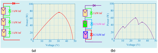
Figure 1.
Partial shading conditions (PSC) effect. (a) Power–voltage (P–V) curve under uniform solar irradiation and temperature and (b) P–V curve under PSC.
3. Transfer Reinforcement Learning with Space Decomposition
The proposed TRL mainly contains two operators, i.e., the RL via uninterrupted interplay with the environment and the knowledge transfer between the previous and new tasks, as clearly illustrated in Figure 2.
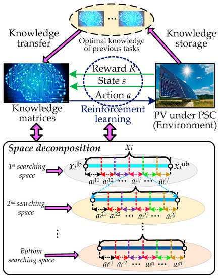
Figure 2.
Principle of transfer reinforcement learning (TRL) with space decomposition.
3.1. Space Decomposition Based Reinforcement Learning
RL is a commonly used machine learning technique, which can acquire new knowledge in a dynamic environment via interaction. Here, the famous RL called Q-learning is adopted to learn the MPPT knowledge. However, if a system needs a high control accuracy, the searching space of the continuous control variable should be divided into a large number of selected actions (e.g., 106 actions for a continuous control variable between 0 to 1). As a result, the conventional Q-learning [28] easily encounters the curse of dimension and a low-efficiency learning rate for selecting an optimal action of a continuous control variable [29].
To handle this problem, the space decomposition is introduced to decompose the large original searching space into multi-layered smaller searching subspaces. As illustrated in Figure 3, the optimization space of the ith controllable variable xi can be decomposed into J smaller searching subspaces in each layer. If the jth action ai1j is selected in the first layer’s searching space, then the agent will seek a more accurate searching space in the corresponding second layer’s searching space. Therefore, the optimization accuracy of the control variable xi can be calculated as
where c represents the number of decomposition layers; and xilb and xiub are the lower and upper bounds of the ith controllable variable, respectively.
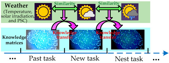
Figure 3.
Knowledge transfer of TRL between two adjacent tasks for maximum power point tracking (MPPT) with PSC.
Based on Equation (4), if the number of actions in each layer is set to be 10 (i.e., J = 10), then the same accuracy (10−6) can be achieved for a continuous control variable between 0 to 1 when c = 6. This means that the number of selected actions can be significantly reduced from 106 to 10. Therefore, the learning rate and control accuracy of Q-learning can be considerably improved, based on the space decomposition.
After selecting all the actions in all the layers, the solution of the controllable variable can be identified as
where and are the lower and upper bounds of the lth layer’s searching space, respectively; while ailj is the jth action in the lth layer’s searching space.
3.2. Knowledge Update
According to the learning mechanism of Q-learning, the knowledge matrix can be updated based on the executed state–action pair with the feedback reward. By combining the space decomposition, the knowledge matrix of each searching space layer can be updated as [28]:
where represents the knowledge matrix of the lth layer’ searching space for the ith controllable variable; is the state–action pair executed at the kth iteration, with k = 1,2,…, kmax; kmax represents the maximum iteration number; α is the knowledge learning factor, with α; γ denotes the discount factor, with γ; Ril is the reward function; and Ail means the action space of the lth layer’s searching space, respectively.
It can be seen from Equation (8) that at each iteration, only one element of each knowledge matrix can be updated since the conventional Q-learning employs a single RL agent for exploration and exploitation in a dynamic environment. Consequently, it will lead to a slow learning rate; thus a high-quality optimal solution cannot be rapidly obtained for a real-time control of PV systems. Hence, a cooperative swarm is employed to further accelerate the learning rate, as it can simultaneously update multiple elements of each knowledge matrix with multiple state-action pairs. Similar to (8), each knowledge matrix of TRL can be updated by [30]
where M represents the population size of the cooperative swarm.
3.3. Exploration and Exploitation
In general, a wide exploration will enhance the possibility of searching a global optimum, but will also consume additional computation time. In contrast, a deep exploitation will enhance the convergence speed, but will easily result in a local optimum in low quality. In order to keep exploitation and exploration in balance, the ε-Greedy rule [31] is adopted to select actions on the basis of the current knowledge matrices, which yields
where q0 is a uniform random number between 0 and 1; ϵ is the rate of exploitation, i.e., the possibility of selecting the greedy action; and arand represents a stochastic action in the action space, i.e., the global search for avoiding a low-quality local optimum, respectively.
3.4. Knowledge Transfer
Through exploiting the optimal knowledge matrices of the previous tasks, the knowledge transfer [32] can approximate the optimal knowledge matrices of a new task, and this is how knowledge transfer works. In this study, the most similar previous task will be chosen for knowledge transfer, based on its similarity with the new task, which can be expressed as
where Qin0 is the approximated optimal knowledge matrices of the ith controllable variable of the new task; Qis* denotes the optimal knowledge matrices of the ith controllable variable of the most similar previous task; Qiinitial represents the initial knowledge matrices of the new task without knowledge transfer; and r represents the comparability between the most similar previous task and the updated task, with , respectively.
4. TRL Design of PV Systems for MPPT
4.1. Control Variable and Action Space
For the purpose of obtaining the GMPP of a PV system, the output voltage Vpv is chosen as the control variable, in which the entire searching space is decomposed into four layers. In each layer, the searching space is uniformly discretized into ten actions within the corresponding range from lower bounds to upper bounds.
4.2. Reward Function
For a given output voltage Vpv, the PV system can generate the corresponding power under the current solar irradiation, temperature, and PSC. In TRL, the higher the quality of the solution is, the larger reward the individual will receive. Based on this rule, the reward function can be designed as [30]:
where is the obtained solution by the mth individual and denotes the explored state–action pairs set of the best individual with the maximum power output at the kth iteration.
4.3. Knowledge Transfer
It is clear that the aforementioned three conditions, e.g., solar irradiation, temperature, and PSC, can be considered as the main similarities between various optimization tasks. On the other hand, the similarity between two adjacent optimization tasks is usually very high, since these weather conditions cannot vary dramatically in a very short time. Hence, the optimal knowledge matrices of the adjacent past task is chosen for knowledge transfer to the new task (See Figure 3), while the similarity described in (11) can be designed as
where and are the temperatures of the new task and the past task, respectively;
4.4. Overall Execution Procedure
For the PV system, the overall flow diagram of TRL to achieve MPPT under PSC is illustrated in Figure 4. Firstly, the original searching space of output voltage is decomposed into a four-layered smaller searching subspace within its corresponding lower bounds and upper bounds. Then, the knowledge transfer between the new task and the past task is implemented according to their similarity of weather conditions. Furthermore, TRL can update the knowledge matrices via multiple explorations and exploitations in the scheduled iterations. At last, for the PV system, the optimal solution (optimal output voltage) can be obtained to achieve MPPT under PSC.
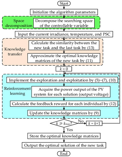
Figure 4.
Overall flow diagram of TRL for MPPT. PSC: Partial Shading Conditions.
5. Case Studies
To further analyze the MPPT practicability of TRL under PSC, it was compared with that of INC [11], GA [15], PSO [16], ABC [17], CSA [18], and TLBO [19], respectively. Four case studies are carried out in this section. Here, each meta-heuristic algorithm shares the same optimization cycle, which is chosen as 0.01 s. Meanwhile, the TRL parameters are given in Table 1.

Table 1.
The parameters of TRL. TRL: Transfer Reinforcement Learning.
For MPPT under PSC, a buck–boost converter is employed, due to its advantages described in reference [33]. Table 2 demonstrates the parameters of the PV system. In addition, the rated values of environment temperature and solar irradiation are set as 25 °C and 1000 W/m2, respectively.
Table 2.
The photovoltaic (PV) system parameters.
5.1. Start-Up Test
The first step to simulate the PSC is to set the solar irradiation of three PV strings to be 200 W/m2, 300 W/m2, and 1000 W/m2, respectively. The online optimization responses of various methods for MPPT are illustrated in Figure 5. It is clear that INC can easily reach the point of steady convergence in far less time than the other methods. However, it has a vital drawback in that it cannot make an effective distinction between GMPP and LMPP, which means it might often be trapped at a low-quality local optimum as it is readily stagnated at an MPP. Generally speaking, due to their significant ability of global searching, other meta-heuristic algorithms can usually find a better quality optimum with larger power and energy. Among them, TRL owns the highest convergence stability as it can avoid a blind/random search by the use of knowledge transfer.
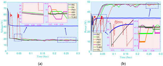
Figure 5.
PV system responses of seven methods obtained on the start-up test. (a) Voltage; (b) Power.
5.2. Step Change in Solar Irradiation with Constant Temperature
As shown in Figure 6, the core process is to impose a set of solar irradiation steps on the PV array, where the step change is applied every second. The temperature is maintained to be constant at 25 °C during the whole test. The online optimization outcomes of various approaches for MPPT with step change solar irradiations are illustrated in Figure 7. It can be found that the obtained results are similar to those of the start-up test. The output power and voltage derived by those meta-heuristic algorithms, except TRL, are relatively prone to volatility if the solar irradiation is not always steady and varies at a dramatic pace. This also verifies that the knowledge transfer can effectively guarantee the convergence stability of TRL, i.e., the control strategies of adjacent optimization tasks only have a slight difference under the same weather conditions.
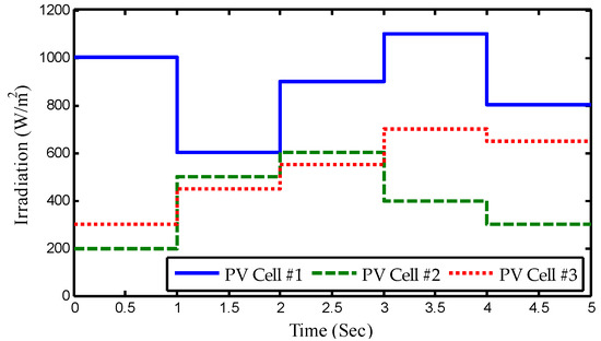
Figure 6.
Step change of solar irradiation with PSC. PSC: Partial Shading Conditions.
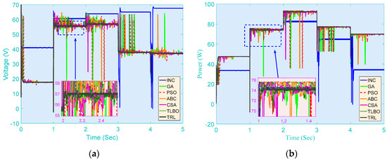
Figure 7.
PV system responses of seven methods obtained on the step change in solar irradiation with constant temperature. (a) Voltage; (b) Power.
5.3. Gradual Change in Both Solar Irradiation and Temperature
Figure 8 and Figure 9 show the procured results of seven algorithms for MPPT when solar irradiation and temperature both change gradually. A conclusion can be drawn that, except for TRL, the other meta-heuristic algorithms are still prone to generating the larger power fluctuations, even when the solar irradiation and temperature change slowly. Due to the beneficial guidance by knowledge transfer, TRL can significantly alleviate the power fluctuations without a blind/random search.
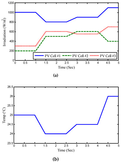
Figure 8.
Gradual change in both solar irradiation and temperature. (a) Irradiation and (b) temperature.
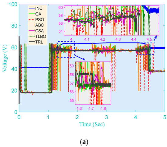
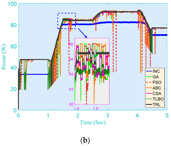
Figure 9.
PV system responses of seven methods obtained on the gradual change in both solar irradiation and temperature. (a) Voltage; (b) Power.
This also reveals that, for real-time MPPT, TRL is capable of speedily seeking an optimum of high quality through the space decomposition on the basis of RL and beneficial knowledge transfer.
5.4. Daily Field Profile of Solar Irradiation and Temperature in Hong Kong
For the purpose of testing the specific practicability of TRL in practical application, the temperature and solar irradiation measured in Hong Kong was used to simulate the PV system for MPPT (See Figure 10 and Figure 11). The metrical data are mainly selected from four representative days of four different seasons in 2016, in which the interval of data is set to 10 min. Note that the randomness and intermittence of solar energy and renewable energy system (RES) [34,35,36,37] is a very common issue usually resulting from uncertain atmospheric conditions.
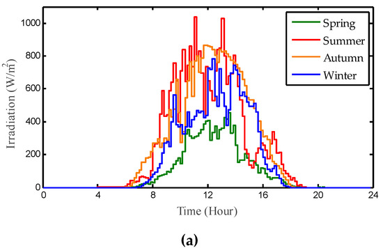
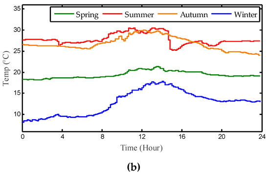
Figure 10.
Daily profile of solar irradiation and temperature in Hong Kong. (a) Irradiation; (b) Temperature.
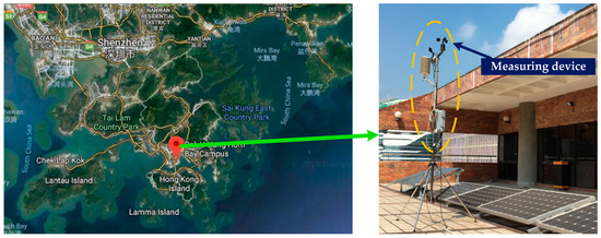
Figure 11.
The detailed geographical position of the measuring device for solar irradiation and temperature.
Figure 12 and Figure 13 demonstrate the output power of seven algorithms for MPPT in different seasons. It can be well illustrated that, compared with INC, in the PV system, all the meta-heuristic algorithms can obtain more output power, where the output energy of TRL reaches 115.52% of that of INC in the spring. That aside, one can derive that although the performances of all meta-heuristic algorithms are comparatively small during the whole simulation period, TRL can still outperform other algorithms, which means that it can always give out the most power in any season.
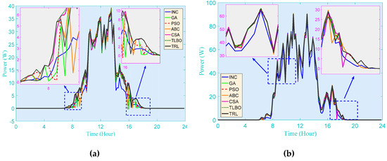
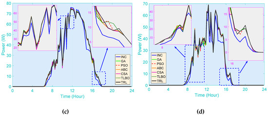
Figure 12.
PV system responses obtained on a typical day in Hong Kong. (a) Spring; (b) summer; (c) autumn; (d) winter.
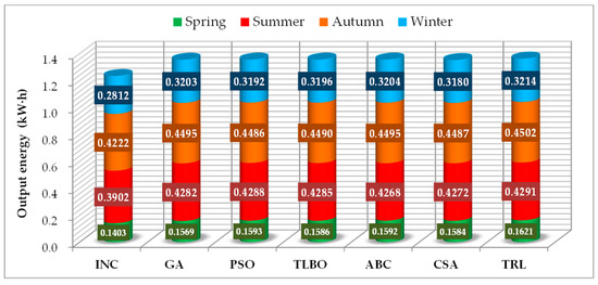
Figure 13.
Statistical results of output energy of the PV system obtained by seven algorithms in different seasons.
6. Conclusions
A novel method called TRL using space decomposition has been proposed in this paper, which is designed for PV systems to obtain the maximum attainable solar energy under PSC, whose contributions can be summarized as follows:
- (1)
- Through space decomposition, TRL can efficiently learn the knowledge for MPPT with PSC in real time; thus a high-quality optimum can be obtained to ensure that the PV system produces more energy under various environmental conditions;
- (2)
- The knowledge transfer can effectively avoid a blind/random search and provide a beneficial guidance to TRL, which results in a fast convergence and a high convergence stability. Therefore, not only can the output power be maximized for the PV system under various scenarios, but the power fluctuation can also be significantly reduced as the weather condition varies;
- (3)
- Compared with the conventional INC and other typical meta-heuristic algorithms, the TRL-based MPPT algorithm can produce the largest amount of output energy in the presence of PSC and other time-varying atmospheric conditions, which can bring about considerable economic benefit for operation in the long term.
Author Contributions
Preparation of the manuscript was performed by M.D., D.L., C.Y., S.L., Q.F., B.Y., and X.Z.
Acknowledgments
The authors gratefully acknowledge the support of ADN Comprehensive Demonstration Project of Smart Grid Application Demonstration Area in Suzhou Industrial Park and Yunnan Provincial Basic Research Project—Youth Researcher Program (2018FD036).
Conflicts of Interest
The authors declare no conflict of interest.
References
- Yang, B.; Yu, T.; Zhang, X.S.; Li, H.F.; Shu, H.C.; Sang, Y.Y.; Jiang, L. Dynamic leader based collective intelligence for maximum power point tracking of PV systems affected by partial shading condition. Energy Convers. Manag. 2019, 179, 286–303. [Google Scholar] [CrossRef]
- Wang, X.T.; Barnett, A. The evolving value of photovoltaic module efficiency. Appl. Sci. 2019, 9, 1227. [Google Scholar] [CrossRef]
- Yang, B.; Yu, T.; Shu, H.C.; Dong, J.; Jiang, L. Robust sliding-mode control of wind energy conversion systems for optimal power extraction via nonlinear perturbation observers. Appl. Energy 2018, 210, 711–723. [Google Scholar] [CrossRef]
- Worighi, I.; Geury, T.; Baghdadi, M.E.; Mierlo, J.V.; Hegazy, O.; Maach, A. Optimal design of hybrid PV-Battery system in residential buildings: End-user economics, and PV penetration. Appl. Sci. 2019, 9, 1022. [Google Scholar] [CrossRef]
- Hyunkyung, S.; Zong, W.G. Optimal design of a residential photovoltaic renewable system in South Korea. Appl. Sci. 2019, 9, 1138. [Google Scholar]
- Yang, B.; Zhong, L.E.; Yu, T.; Li, H.F.; Zhang, X.S.; Shu, H.C.; Sang, Y.Y.; Jiang, L. Novel bio-inspired memetic salp swarm algorithm and application to MPPT for PV systems considering partial shading condition. J. Clean. Prod. 2019, 215, 1203–1222. [Google Scholar] [CrossRef]
- Gulkowski, S.; Zdyb, A.; Dragon, P. Experimental efficiency analysis of a photovoltaic system with different module technologies under temperate climate conditions. Appl. Sci. 2019, 9, 141. [Google Scholar] [CrossRef]
- Wu, Z.; Yu, D. Application of improved bat algorithm for solar PV maximum power point tracking under partially shaded condition. Appl. Soft Comput. 2018, 62, 101–109. [Google Scholar] [CrossRef]
- Tanaka, T.; Toumiya, T.; Suzuki, T. Output control by hill-climbing method for a small scale wind power generating system. Renew. Energy 2014, 12, 387–400. [Google Scholar] [CrossRef]
- Mohanty, S.; Subudhi, B.; Ray, P.K. A grey wolf-assisted Perturb & Observe MPPT algorithm for a PV system. IEEE Trans. Energy Convers. 2017, 32, 340–347. [Google Scholar]
- Zakzouk, N.E.; Elsaharty, M.A.; Abdelsalam, A.K.; Helal, A.A. Improved performance low-cost incremental conductance PV MPPT technique. IET Renew. Power Gener. 2016, 10, 561–574. [Google Scholar] [CrossRef]
- Sher, H.A.; Murtaza, A.F.; Noman, A.; Addoweesh, K.E.; Al-Haddad, K.; Chiaberge, M. A new sensorless hybrid MPPT algorithm based on fractional short-circuit current measurement and P&O MPPT. IEEE Trans. Sustain. Energy 2015, 6, 1426–1434. [Google Scholar]
- Huang, Y.P. A rapid maximum power measurement system for high-concentration Photovoltaic modules using the fractional open-circuit voltage technique and controllable electronic load. IEEE J. Photovolt. 2014, 4, 1610–1617. [Google Scholar] [CrossRef]
- Rezk, H.; Fathy, A.; Abdelaziz, A.Y. A comparison of different global MPPT techniques based on meta-heuristic algorithms for photovoltaic system subjected to partial shading conditions. Renew. Sustain. Energy Rev. 2017, 74, 377–386. [Google Scholar] [CrossRef]
- Messai, A.; Mellit, A.; Guessoum, A.; Kalogirou, S.A. Maximum power point tracking using a GA optimized fuzzy logic controller and its FPGA implementation. Sol. Energy 2011, 85, 265–277. [Google Scholar] [CrossRef]
- Babu, T.S.; Rajasekar, N.; Sangeetha, K. Modified Particle Swarm Optimization technique based Maximum Power Point Tracking for uniform and under partial shading condition. Appl. Soft Comput. 2015, 34, 613–624. [Google Scholar] [CrossRef]
- Benyoucef, A.S.; Chouder, A.; Kara, K.; Silvestre, S.; Sahed, O.A. Artificial bee colony based algorithm for maximum power point tracking (MPPT) for PV systems operating under partial shaded conditions. Appl. Soft Comput. 2015, 32, 38–48. [Google Scholar] [CrossRef]
- Ahmed, J.; Salam, Z. A maximum power point tracking (MPPT) for PV system using Cuckoo search with partial shading capability. Appl. Energy 2014, 119, 118–130. [Google Scholar] [CrossRef]
- Rezk, H.; Fathy, A. Simulation of global MPPT based on teaching-learning-based optimization technique for partially shaded PV system. Electr. Eng. 2017, 99, 847–859. [Google Scholar] [CrossRef]
- Javed, M.Y.; Murtaza, A.F.; Ling, Q.; Qamar, S.; Gulzar, M.M. A novel MPPT design using generalized pattern search for partial shading. Energy Build. 2016, 133, 59–69. [Google Scholar] [CrossRef]
- Titri, S.; Larbes, C.; Toumi, K.Y.; Benatchba, K. A new MPPT controller based on the Ant colony optimization algorithm for Photovoltaic systems under partial shading conditions. Appl. Soft Comput. 2017, 58, 465–479. [Google Scholar] [CrossRef]
- Silver, D.; Huang, A.; Maddison, C.J.; Guez, A.; Sifre, L.; Van Den Driessche, G.; Dieleman, S. Mastering the game of Go with deep neural networks and tree search. Nature 2016, 529, 484–489. [Google Scholar] [CrossRef] [PubMed]
- Sutton, R.S.; Barto, A.G. Reinforcement Learning: An Introduction; MIT Press: Cambridge, MA, USA, 1998. [Google Scholar]
- Qi, J.; Zhang, Y.; Chen, Y. Modeling and maximum power point tracking (MPPT) method for PV array under partial shade conditions. Renew. Energy 2014, 66, 337–345. [Google Scholar] [CrossRef]
- Lalili, D.; Mellit, A.; Lourci, N.; Medjahed, B.; Berkouk, E.M. Input output feedback linearization control and variable step size MPPT algorithm of a grid-connected photovoltaic inverter. Renew. Energy 2011, 36, 3282–3291. [Google Scholar] [CrossRef]
- Lalili, D.; Mellit, A.; Lourci, N.; Medjahed, B.; Boubakir, C. State feedback control and variable step size MPPT algorithm of three-level grid-connected photovoltaic inverter. Sol. Energy 2013, 98, 561–571. [Google Scholar] [CrossRef]
- Chen, K.; Tian, S.; Cheng, Y.; Bai, L. An improved MPPT controller for photovoltaic system under partial shading condition. IEEE Trans. Sustain. Energy 2017, 5, 978–985. [Google Scholar] [CrossRef]
- Watkins, J.C.H.; Dayan, P. Q-learning. Mach. Learn. 1992, 8, 279–292. [Google Scholar] [CrossRef]
- Er, M.J.; Deng, C. Online tuning of fuzzy inference systems using dynamic fuzzy Q-learning. IEEE Trans. Syst. Man Cybern. Part B 2004, 34, 1478–1489. [Google Scholar] [CrossRef]
- Zhang, X.; Yu, T.; Yang, B.; Cheng, L. Accelerating bio-inspired optimizer with transfer reinforcement learning for reactive power optimization. Knowl. Based Syst. 2017, 116, 26–38. [Google Scholar] [CrossRef]
- Bianchi, R.A.C.; Celiberto, L.A.; Santos, P.E.; Matsuura, J.P.; Lopez de Mantaras, R. Transferring knowledge as heuristics in reinforcement learning: A case-based approach. Artif. Intell. 2015, 226, 102–121. [Google Scholar] [CrossRef]
- Pan, J.; Wang, X.; Cheng, Y.; Cao, G. Multi-source transfer ELM-based Q learning. Neurocomputing 2014, 137, 57–64. [Google Scholar] [CrossRef]
- Ishaque, K.; Salam, Z.; Amjad, M.; Mekhilef, S. An improved particle swarm optimization (PSO)-based MPPT for PV with reduced steady-state oscillation. IEEE Trans. Power Electron. 2012, 27, 3627–3638. [Google Scholar] [CrossRef]
- Li, G.D.; Li, G.Y.; Zhou, M. Model and application of renewable energy accommodation capacity calculation considering utilization level of interprovincial tie-line. Prot. Control Mod. Power Syst. 2019, 4, 1–12. [Google Scholar] [CrossRef]
- Tummala, S.L.V.A. Modified vector controlled DFIG wind energy system based on barrier function adaptive sliding mode control. Prot. Control Mod. Power Syst. 2019, 4, 34–41. [Google Scholar]
- Faisal, R.B.; Purnima, D.; Subrata, K.S.; Sajal, K.D. A survey on control issues in renewable energy integration and microgrid. Prot. Control Mod. Power Syst. 2019, 4, 87–113. [Google Scholar]
- Dash, P.K.; Patnaik, R.K.; Mishra, S.P. Adaptive fractional integral terminal sliding mode power control of UPFC in DFIG wind farm penetrated multimachine power system. Prot. Control Mod. Power Syst. 2018, 3, 79–92. [Google Scholar] [CrossRef]


© 2019 by the authors. Licensee MDPI, Basel, Switzerland. This article is an open access article distributed under the terms and conditions of the Creative Commons Attribution (CC BY) license (http://creativecommons.org/licenses/by/4.0/).