Article

Trajectory Planning and Optimization for a Par4 Parallel Robot Based on Energy Consumption

1
School of Mechano-Electronic Engineering, Xidian University, Xi’an 710000, China
2
School of Physics and Electronic Engineering, Xianyang Normal University, Xianyang 712000, China
*
Author to whom correspondence should be addressed.
Appl. Sci. 2019, 9(13), 2770; https://doi.org/10.3390/app9132770
Submission received: 7 May 2019 / Revised: 13 June 2019 / Accepted: 4 July 2019 / Published: 9 July 2019

Abstract

:
A study on trajectory planning and optimization for a Par4 parallel robot was carried out, based on energy consumption in high-speed picking and placing. In the end-effector operating space of the Par4 parallel robot, the rectangular transition of the pick-and-place trajectory was rounded by a Lamé curve. A piecewise design method was adopted to accomplish trajectory shape planning for displacement, velocity and acceleration. To make the Par4 robot’s end run more smoothly and to reduce residual vibration, asymmetric fifth-order and sixth-order polynomial motion laws were employed. With the aim of reaching the minimum mechanical energy consumption for the Par4 parallel robot, the recently proposed Grey Wolf Optimizer (GWO) algorithm was adopted to optimize the planning trajectory. The validity of the design method was verified by experiments, and it was found that the minimum mechanical energy consumption of the optimal trajectory planned under the law of fifth-order polynomial motion is lower than that of sixth-order polynomial motion. In addition, the experiments also revealed the optimal values of Parameters e and f, which were the parameters of the Lamé curve function. Parameter e can be calculated as half the pick-up span for the minimum mechanical energy consumption, unlike parameter f, whose optimal value depends on specific circumstances such as the pick-and-place coordinates and the pick-up height.

1. Introduction

In recent years, parallel robots have been widely developed for their optimal dynamic properties [1,2], especially parallel robots with lower mobility such as Delta, H4, X4, and Par4. [3,4]. At present, parallel robots are widely used in high-precision fields [5,6,7] such as aviation manufacturing, electronic packaging, and 3D printing.
A reasonable trajectory planning of a robot can help it not only to perform the desired tasks with satisfactory performance [8], but it is also conducive to improving efficiency [9], reducing energy consumption, and extending the operating life [10,11]. At present, there are many studies on robot trajectory planning, such as in [12] (point-to-point dynamic trajectory planning was carried out for six degree-of-freedom (six-DOF) parallel robots, attaining good effects), [13] (point-to-point dynamic trajectory planning was carried out for three degree-of-freedom (three-DOF) parallel robots, also attaining good effects), and [14] (a new s s ¨ plane path method was adopted to design a dynamic feasible point-to-point path and periodic trajectories, based on the forces of geometric constraints).
In general, robot trajectory planning can be either on the end-effector or on the joint level [15]. If it is done on the joint level, the end-effector trajectory of the robot should be mapped to the joint motion trajectory based on inverse kinematics [16], then only the joint motion needs to be controlled, and the result of the motion planning is only evaluated at each joint [17]. If done on the end-effector level, the motion planning is directly on the end-effector, and the evaluation and control are all applied on the end-effector [18]. In [19], trajectory planning for a Delta parallel robot was carried out on the end-effector and on the joint level, respectively. Through comparative analysis, it was found that the trajectory planning on the joint level could effectively reduce the maximum torque of the motor and the vibration amplitude of the robot end in the movement process. In view of this, from the lower rated torque of the motor and the lower vibration amplitude of the robot end of view, in this paper the trajectory planning of a Par4 parallel robot will be carried out on the joint level, i.e., first, we will design the shape of movement track and the motion law on the end-effector level, then, the motion feature of the end-effector will be mapped to the joint space, and the follow-up evaluation and control will all be conducted at each joint.
Trajectory planning and trajectory optimization are often carried out simultaneously, and the common optimization objectives are minimum time [20], minimum energy [21], minimum pulsation [22], and maximum load-carrying capacity [23]. The minimum time optimization, directly associated with the production efficiency of the robot, was the first of these objectives to be considered, having been widely applied. For instance, in [24], considering three different types of constraints, smooth joint trajectories were constructed with the cubic polynomial function, a genetic algorithm procedure with parallel-populations was applied for the purpose of minimizing time, and finally, the validity of the method was verified; in [25], a time-optimal trajectory planning method was proposed, based on quintic Pythagorean Hodograph (PH) curves, in order to realize a smooth and high-speed operation of a Delta parallel robot. If we blindly pursue the minimum execution time at actual operation, it will easily lead to the discontinuity of torque and acceleration. Energy consumption is also one of the most concerning indexes of parallel robots, and especially when the energy source of the robot system is limited, it is more meaningful to study the minimum energy consumption than other optimization objectives. At present, some researchers have done trajectory planning for robots with minimal energy consumption. For example, in [26], a method of trajectory planning with minimum energy damping was proposed for a flexible-base robot, considering the point-to-point motion task. The maximum residual vibration amplitude and operating energy were taken as objective functions, and the radial basis function networks (RBFNs) were optimized using non-dominated sorting genetic algorithms-II (NSGA-II). In [27], a design method based on the concept of universal redundancy was proposed to improve the dynamic performance of the mechanism. After the servo motor’s motion path was divided into multiple segments, the trajectory planning of each segment was designed, respectively, applying the law of polynomial motion. Some polynomial parameters, as well as the speed and acceleration of the working point, should be selected with the minimal optimization for energy and vibration force, based on the genetic algorithm. The validity of the method was verified by experiments, but since there were many parameters to be optimized, it was easy to fall into the local optimum. An underactuated self-reconfigurable robot with active and passive joints was designed in [28], and reconfiguration planning and scheduling were carried out with the aim of minimizing energy consumption based on the genetic algorithm. In [29], three trajectories were designed based on a model of an underwater robot, based on minimum energy, minimum turbulence, and minimum torque change rate, respectively. Finally, the fourth trajectory with minimal energy based on the genetic algorithm was planned, in which a polynomial approximates the time histories of the trajectory in joint space; the running time and the coordinates of an intermediate point were taken as the object to be optimized, and the quartic polynomial was selected as its motion law. The advantage of this method was that it was not reliant on an accurate mathematical model; however, since the intermediate point was obtained by random search, the shape of the trajectory could not be well controlled. At present, to the best of our knowledge, no trajectory planning involving energy consumption has yet been elaborated for a Par4 parallel robot. In this paper, in order to study the trajectory planning and energy consumption of the Par4 parallel robot, the minimum energy consumption was taken as the optimized object.
High-speed pick-and-place operation is one of the main working modes of parallel robots [30,31], and a gate-shaped trajectory is usually adopted, as shown in Figure 1. In the figure, A and H are the pick-and-place endpoints, B, C, E, F and G the intermediate points on the pick-and-place track, H a is the vertical displacement, also known as pick-up height, and B a is the horizontal displacement, also known as pick-up span. The trajectory is symmetric with respect to the dot line MN.
A polynomial of third order or more, a modified trapezoid and Bang-Bang algorithms are usually applied as the law of motion [32,33]. Due to the right-angle connection of the conventional gate trajectory (as shown by the solid line in Figure 1), it is easy to cause the discontinuity of the motor’s speed and acceleration in the process of movement, which leads to severe mechanical vibration in the robot. Therefore, a smooth transition is often applied instead of the right-angle connection, as shown by the dotted line in Figure 1. The ideal transition curve should meet the criterion of continuous curvature. In [34], taking the five-bar mechanism as the object, a variety of motion trajectories were compared and analyzed, and the results show that the Lamé curve is better than the others in terms of residual vibration and the precision of the final position. However, there was no optimization research about the trajectory with the Lamé curve in [34]. Based on this, in this paper, for the design of trajectory planning and optimization of the Par4 parallel robot, the Lamé curve was calculated for a smooth transition of the pick-and-place path; some comparisons were made between the fifth- and sixth-order polynomial motion laws; and Grey Wolf Optimizer (GWO) was selected for optimizing the Lamé curve parameters with minimum mechanical energy consumption.

2. Par4 Parallel Robot

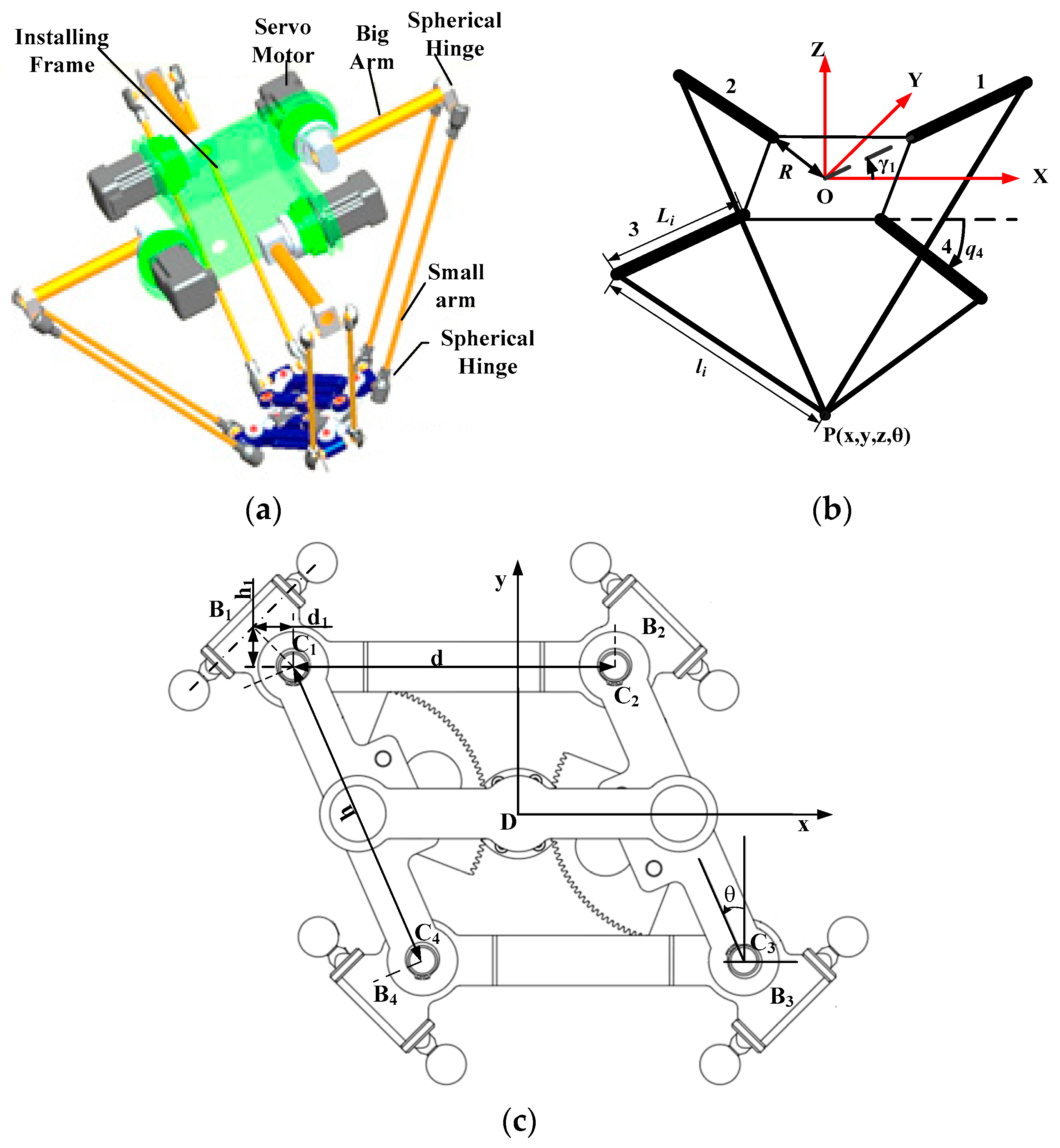
The structure of the 4-Dof Par4 parallel robot is shown in Figure 2a, consisting of three parts: (1) A fixed platform mainly composed of the mounting frame and the servo motor and reducer component; (2) a moving platform where the actuator is located; (3) four symmetric branched chains connecting the big arm and small arm by a spherical hinge. The simplified structure diagram for the Par4 robot is shown in Figure 2b, in which the moving platform has been simplified to Particle P. The OXYZ coordinate system is established on the fixed platform, where O is the fixed platform center. In Figure 2b, L i and l i are the lengths of the big arm and small arm, respectively, R is the distance from the origin O to the big arm revolute center, which is called the big arm revolute radius for short in the following article, q i ( i = 1 , 2 , 3 , 4 ) is the rotation angle of each big arm (only q 4 is marked in Figure 2b), and γ i ( i = 1 , 2 , 3 , 4 ) is the angle from the axial direction from each big arm base to the X axis ( γ i = ( 2 i 1 ) π / 4 ). The pose of the moving platform (Particle P) is described as ( x , y , z , θ ) , where x , y and z are the coordinate values in the OXYZ system, and θ is the rotation angle of the moving platform, as shown in Figure 2c which is the top view of the end-effector. For easier description, the local reference coordinate xDy system is established and is shown in Figure 2c, where D is the moving platform center. In Figure 2c,d,h are the moving platform lengths along the x and y axes, respectively; B i is the center of the support where the two ball hinges connecting the ith small arm with the moving platform are located; the moving platform can be considered a hinged parallelogram, as shown in Figure 2c; C i is the pivot of its ith hinge, which can be considered as the ith vertex of the hinged parallelogram; d i is the distance along the x axis between B i and C i ; and h i is the distance along the y axis between B i and C i , here i = 1 , 2 , 3 , 4 .

2.1. Inverse Kinematics of the Par4 Parallel Robot

According to the Par4 parallel robot structure, the inverse kinematic rotation angle of each big arm can be obtained as shown in Equation (1):
q i = 2 arctan ( I i I i 2 K i 2 + J i 2 K i J i ) , i = 1 , 2 , 3 , 4 .
Here, I i = L i z , K i = ( a i 2 + b i 2 + L i 2 l i 2 + z 2 ) / 2 , J i = L i ( a i cos γ i + b i sin γ i ) , a i = x ε i h sin θ + ξ i d / 2 + ς i d i R cos γ i , b i = y + ε i h cos θ + σ i h i R sin γ i , ε = [ ε 1 , ε 2 , ε 3 , ε 4 ] = [ 1 , 1 , 1 , 1 ] , ξ = [ ξ 1 , ξ 2 , ξ 3 , ξ 4 ] = [ 1 , 1 , 1 , 1 ] , ς = [ ς 1 , ς 2 , ς 3 , ς 4 ] = [ 1 , 1 , 1 , 1 ] , and σ = [ σ 1 , σ 2 , σ 3 , σ 4 ] = [ 1 , 1 , 1 , 1 ] .
Given the spatial trajectory of the robot end-effector, the angular displacement of each driving mechanism can be obtained through the inverse kinematic equations, as in Equation (1). Accordingly, if the robot is driven with this obtained angular displacement law, the expected end-effector spatial trajectory will be achieved [35].

2.2. Dynamic Equation of the Par4 Parallel Robot

First, some simplifications of the system structure have been done, i.e., (1) the mass of the big arm ( m b ) is simplified to the geometric center of the big arm; (2) the small arm is equivalent to a bar, and the mass of the two rods of the small arm ( m s and m s ) are equivalent to both ends of the bar. Regardless of the influence of internal stress of the Par4 parallel robot, the dynamic equation of Par4 parallel robot can be obtained, as follows:
τ = J T M p f ( X ¨ + g ) + I q ¨ + f s s i g n ( q ˙ ) + f v q ˙ + M n L i cos q
where τ = [ τ 1 , τ 2 , τ 3 , τ 4 ] T , τ i ( i = 1 , 2 , 3 , 4 ) is the drive torque of each joint, J is the kinematics Jacobian matrix of the Par4 parallel robot. X = [ x , y , z , θ ] T , X ¨ is the second derivative of X , namely the acceleration of the moving platform end; q = [ q 1 , q 2 , q 3 , q 4 ] T , q ˙ and q ¨ are the first and second derivative of q respectively, representing the angular velocity vector and the angular acceleration vector; g is the gravitational acceleration vector, g = [ 0 , 0 , 9.8 , 0 ] T , and M p f is the mass matrix of the actuator, which can be represented as
M p f = d i a g ( M p f e , M p f e , M p f e , m 44 )
where M p f e = m c + m d + 4 m s , m 44 = 2 ( m d / 2 + 2 m s ) ( h / 2 ) 2 , m c is the load mass of the moving platform, m s the mass of a small arm, and m d the mass of the moving platform.
In Equation (2), I = I b i n + I b + I b o u t , I b i n is the inertia matrix of the inner connections, I b the big arm rotational inertia matrix about its active joint, I b o u t the total rotational inertia matrix of the small arm and the big arm end connections about the active joint, i.e., I = ( m e n d + m s ) L i 2 E ( 4 ) , where m e n d is the mass of the big arm end connections. s i g n ( q ˙ ) = [ s i g n ( q ˙ 1 ) , s i g n ( q ˙ 2 ) , s i g n ( q ˙ 3 ) , s i g n ( q ˙ 4 ) ] T is the Sign function vector of the active joint angular velocity, f s the Coulomb friction factor, f v the viscous friction factor. It should be mentioned that since the speed of the motor (connected to the harmonic reducer with high deceleration ratio) is higher, the frictions of all the spherical hinges have been ignored. M n = m b / 2 + m e n d + m s , where m b is the mass of a big arm, and cos q is the cosine vector of the active joint rotation angle.

3. Trajectory Planning of the Par4 Parallel Robot

The following detailed trajectory planning is carried out by constructing the Lamé curve as a smooth transition curve.

3.1. Trajectory Planning Based on Lamé Curve

The general expression of the Lamé curve is
( u e ) n + ( w f ) n = 1    e > 0 , f > 0 , n = 1 , 2 ,
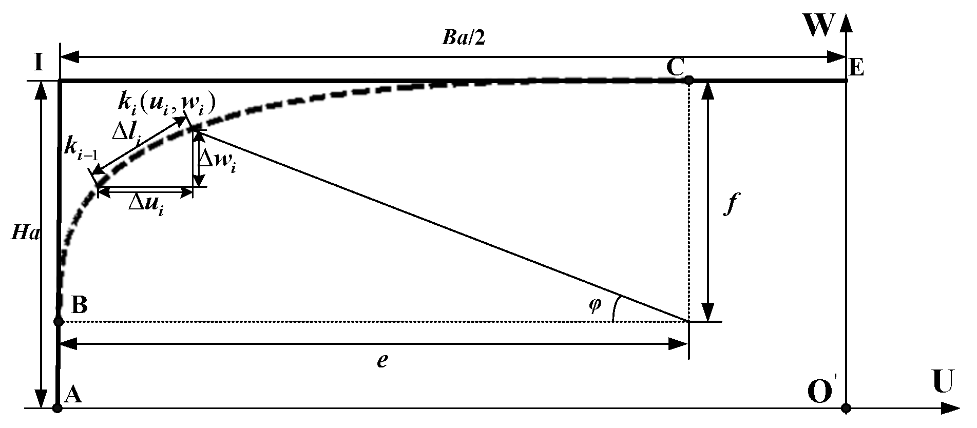
It is known that when n 3 , the points B and C, where the Lamé curve and the line cross, will be continuous [36]. For simplicity, let us take n = 3 . The half-way trajectory is shown in Figure 3, where the dotted line is the trajectory of the Lamé curve.
In Figure 3, AB is the vertical movement, BC is the Lamé curve movement (shown in dotted lines in Figure 3), and CE is the horizontal movement. H a is the pick-up height, and the horizontal length of IE is half the pick-up span B a . Setting up the local plane coordinate system U O W , the geometric meaning of parameters e and f in Equation (4) are shown in Figure 3. φ is the turned angle from the starting point B to the point k i ( u i , w i ) on the Lamé curve, which is noted clearly in Figure 3. The turned angle from the starting point B to the point C is π / 2 .
The arc length of the curve from B to C is
l B C = 0 π 4 ( 1 + tan 2 φ ) e 2 tan 4 φ + f 2 ( 1 + tan 3 φ ) 4 / 3 d φ + 0 π 4 ( 1 + tan 2 φ ) f 2 tan 4 φ + e 2 ( 1 + tan 3 φ ) 4 / 3 d φ .
In the local coordinate system U O W , the coordinates of any point on the Lamé curve can be expressed as Equation (6), based on the turned angle φ :
{ u ( φ ) = 2 e + ( 2 e B a ) ( 1 + tan 3 φ ) 1 / 3 2 ( 1 + tan 3 φ ) 1 / 3 w ( φ ) = f tan φ + ( H a f ) ( 1 + tan 3 φ ) 1 / 3 ( 1 + tan 3 φ ) 1 / 3

3.2. Space-Path Coordinate Transform

For the convenience of our study, it is necessary to transform the spatial gate-shaped path in the OXYZ coordinate system into the one seen in the U O W plane local coordinate system. Assuming the pick-up endpoints have the same spatial Z-axis coordinate value, the transformation from the OXYZ coordinate system to the U O W plane local coordinate system only needs to take the translation of the origin and the rotation transformation along the X axis into consideration. The coordinates ( x , y , z ) of any spatial point in the OXYZ coordinate system will be marked as ( u , w ) in the U O W plane local coordinate system after the transition, which can be described as Equation (7).
[ x y z 1 ] = Q [ u 0 w 1 ] = [ λ 11 λ 12 λ 13 λ 14 λ 21 λ 22 λ 23 λ 24 λ 31 λ 32 λ 33 λ 34 λ 41 λ 42 λ 43 λ 44 ] [ u 0 w 1 ]
where Q is the transformation matrix from the U O W coordinates to the OXYZ coordinates, and Q 1 is the transformation matrix from the OXYZ coordinates to the U O W coordinates.

3.3. Motion Law Planning

In this section, the motion law planning of the Par4 robot in the operating space is studied, which focuses on the displacement, velocity, and acceleration of the robot’s end-effector. In order to ensure the smooth running of the robot end and to reduce residual vibration, a polynomial of fifth order or more is employed for the displacement planning. The higher the order is, the more complex the calculation will be. Thus, for simplicity, fifth- and sixth-order polynomials are selected here for displacement planning.

3.3.1. Polynomial Displacement Planning

  • Quintic Polynomial Displacement Planning
For the stable operation of the robot end, the maximum acceleration is set at T/4 time, where T is the pick-and-place period. The expressions of the quintic polynomial displacement and maximum acceleration are obtained as Equations (8) and (9), by analyzing the initial and final displacement boundary conditions, velocity boundary conditions and acceleration boundary conditions:
s ( t ) = a max T 2 ( 6 τ 5 15 τ 4 + 10 τ 3 ) / 5.625
a max = 5.625 S a / T 2
where τ = t / T , t is the current time; S a is the total pick-up displacement, and here S a = 2 ( H a f e + l B C ) + B a .
  • Sextic Polynomial Displacement Planning
To reduce residual vibration at the falling point of the robot end, the proportion of the acceleration time and deceleration time is set as 4:6 in the sextic polynomial motion law, meaning that the maximum velocity is at 2T/5 time when the acceleration is zero, a ( 2 T / 5 ) = 0 . Then, the expression of displacement can be described as in Equation (10).
s ( t ) = S a ( 10 τ 6 + 36 τ 5 45 τ 4 + 20 τ 3 )
It should be remembered that both the quintic and the sextic polynomial displacement planning expressions are asymmetric.

3.3.2. Piecewise Motion Planning Based on the Lamé Curve

Based on Figure 2 and Figure 3, there are five segments in the gate-shaped pick-and-place movement: The AB segment rising vertically, the BC segment rising along the Lamé curve, the CF segment moving horizontally, the FG segment falling along the Lamé curve and the GH segment falling vertically. Due to the symmetry of the motion trajectory, the following section will mainly study the motion planning of the AB segment, BC segment, and CF segment in the U O W plane local coordinate system, and finally convert the planning to the space coordinate OXYZ.
  • AB Segment Motion Planning
The displacement range is 0 s ( t ) < ( H a f ) , with vertical motion only. The spatial coordinates of point A are set as ( x A , y A , z A ) , and the current time is denoted as t i , so, the displacement, velocity and acceleration laws in the space coordinate OXYZ can be shown in Equations (11)–(13):
[ x i y i z i ] = [ x A y A z A + s ( t i ) ]
[ v x i v y i v z i ] = [ 0 0 s ( t i ) ]
[ a x i a y i a z i ] = [ 0 0 s ( t i ) ] .
2.
BC Segment Motion Planning
  • Displacement Planning
When the displacement is taken as ( H a f ) s ( t ) < ( H a f ) + l B C , it moves along the Lamé curve. Taking the previous running point to be k i 1 , the current running point is k i , as indicated in Figure 3. The key is to calculate the interpolation values Δ u i and Δ w i . In Figure 3, there is the increment of arc length Δ l i = s ( t i ) s ( t i 1 ) , in which t i represents the present time, and t i 1 the previous time. According to Equation (4), Equation (14) is deduced:
u i ( w ) = ( w i 2 e 3 ) / ( u i 2 f 3 )
When the interpolation time is Δ t i 0 , then Δ l i 0 . The approximate arc differential calculation formula can be obtained as in Equation (15):
Δ w i Δ l i / 1 + [ u i ( w ) ] 2 .
Thus,
w i = w i 1 + Δ w i .
The following can be obtained from Equations (4) and (16):
u i = e [ 1 ( w i / f ) 3 ] 1 / 3
Δ u i = u i u i 1 .
According to the analysis above, to avoid u i ( w ) when k i is approaching the W axis, w i ( u ) = ( u i 2 f 3 ) / ( w i 2 e 3 ) can be calculated first with Equation (4), and in the same way, Δ u i can be calculated first, before calculating u i , w i , and Δ w i in turn. There is a strong duality between the two calculated methods. In order to reduce calculation errors, when ( H a f ) s ( t ) < ( H a f ) + l B C / 2 , the former method is adopted; when ( H a f ) + l B C / 2 s ( t ) < ( H a f ) + l B C , the latter method is adopted.
The coordinate transformation can be attained as
[ x i y i z i ] = [ λ 11 λ 13 λ 21 λ 23 λ 31 λ 33 ] [ u i w i ] + [ λ 14 λ 24 λ 34 ]
If X i = [ x i y i z i ] , Q 1 = [ λ 11 λ 13 λ 21 λ 23 λ 31 λ 33 ] , Q 2 = [ λ 14 λ 24 λ 34 ] T , U i = [ u i w i ] T , Equation (19) can be denoted as X i = Q 1 U i + Q 2 .
  • Speed Planning
When Δ t i 0 , Δ l i 0 , Δ l i Δ u i 2 + Δ w i 2 , then
v u i s ( t i ) Δ u i Δ u i 2 + Δ w i 2 = s ( t i ) Δ u i Δ l i
v w i s ( t i ) Δ w i Δ u i 2 + Δ w i 2 = s ( t i ) Δ w i Δ l i .
The velocities converted to the robot’s end space coordinate OXYZ are
[ v x i v y i v z i ] T = Q 1 [ v u i v w i ] T .
  • Acceleration Planning
The acceleration along the U axis can be calculated as follows:
u ( t ) = d d t u ( t ) = d d t ( u ( φ ) φ ( t ) ) = u ( φ ) [ φ ( t ) ] 2 + u ( φ ) φ ( t ) .
Similarly, the acceleration calculation formula along the W axis can be obtained as
w ( t ) = w ( φ ) [ φ ( t ) ] 2 + w ( φ ) φ ( t ) .
Here, all of u ( φ ) , u ( φ ) , w ( φ ) and w ( φ ) can be calculated by Equation (6), and the calculation of φ ( t ) and φ ( t ) will be derived as follows:
Since s ( t ) = s ( φ ) φ ( t ) , and the motion of the Lamé curve shown in Figure 3 is in the rising state, i.e., s ( φ ) > 0 , then φ ( t ) can be calculated as Equation (25):
φ ( t ) = s ( t ) s ( φ ) = s ( t ) [ u ( φ ) ] 2 + [ w ( φ ) ] 2 .
Thus, φ ( t ) can be calculated by performing the derivation of Equation (25) with respect to the variable t.
The acceleration converted to the robot end space coordinate OXYZ is
[ a x i a y i a z i ] T = Q 1 [ a u i a w i ] T = Q 1 [ u ( t i ) w ( t i ) ] T .
3.
CF Segment Motion Planning
When the displacement is taken as ( H a f + l B C ) s ( t ) < ( H a f + l B C + B a 2 e ) , the motion of the CF segment is a plane horizontal movement, and in the U O W coordinate system, there are the following equations: Δ u i = Δ l i = s ( t i ) s ( t i 1 ) , Δ w i = 0 , v u i = s ( t i ) , v w i = 0 , a u i = s ( t i ) , and a w i = 0 .
Taking the coordinate of point C in the U O W coordinate system as ( u C , w C ) , then, u i = u i 1 + Δ u i = u i 1 + Δ l i , and w i = w i 1 = w C .
The planning converted to the robot end space OXYZ is
{ [ x i y i z i ] T = Q 1 [ u i w C ] T + Q 2 [ v x i v y i v z i ] T = Q 1 [ s ( t i ) 0 ] T [ a x i a y i a z i ] T = Q 1 [ s ( t i ) 0 ] T .
4.
Other Segment Motion Planning
Due to the left–right symmetry of the gate-shaped trajectory, the FG segment’s motion is identical to the BC segment’s, and the GH segment’s motion to the AB segment’s, so they will be not elaborated here.
According to the motion planning described above, the interpolation displacement, velocity, and acceleration of the gate-shaped trajectory at each moment can be obtained based on the Lamé curve, and then the rotation angle of each driving unit can be obtained through the inverse kinematic equation analysis, so that the desired trajectory planning can be achieved.

4. Trajectory Optimization Based on GWO

Although the trajectory shape and motion law of the Par4 parallel robot have been planned in the previous sections, the problem of parameter selection for the Lamé curve remains unresolved. Previously, the parameters of the Lamé curve have mainly been determined in the planning process through prior knowledge, and certainly there are some optimization designs done already, such as the method for a Delta parallel robot in [37], which is a brute force optimization method where the parameters of the Lamé curve were traversed at a step length of 1 mm, thus causing not only a heavy workload but also a large degree of optimization error. Therefore, in this paper, we adopt the recently proposed Grey Wolf Optimizer (GWO) to achieve the trajectory optimization with the target of minimal energy consumption for the Par4 parallel robot. In this section, the GWO algorithm is first introduced, and then the trajectory optimization method is elaborated.

4.1. Grey Wolf Optimizer

The GWO algorithm is a new intelligent algorithm, proposed in 2014 [38]. Because of its features of simple operational structure, high search efficiency, and ease of understanding and programming, it has been widely employed in all walks of life since it was proposed [39,40,41].
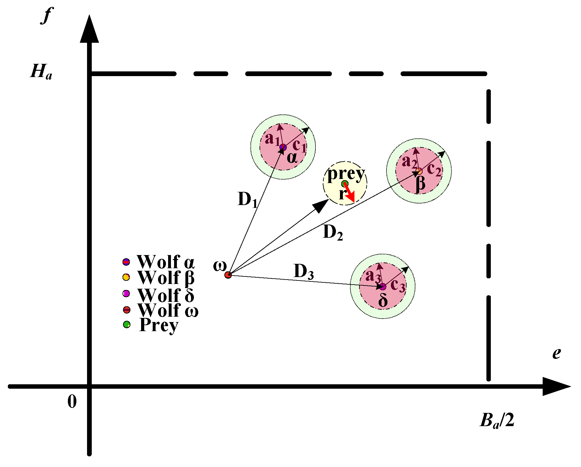
The GWO algorithm aims to simulate the group hunting behavior of grey wolves [38]. In GWO, the prey represents the optimal solution, and the process of optimization can be understood as catching the prey. Generally, there are three grey wolves in leadership roles, named Wolf α, Wolf β and Wolf δ, and there are many searching wolves, all called Wolf ω, whose number is often in dozens. During the process of catching the prey, Wolf α is the wolf closest to the prey, Wolf β the further away, and Wolf δ further away again. The positions of the three leader grey wolves are always taken as a reference for Wolf ω to carry out the hunting search behavior. Until all Wolves ω complete the hunting search behavior with their own positions updated, the position of Wolf α, Wolf β or Wolf δ can be updated as long as the solution of Wolf ω is better than theirs. In each iteration, Wolf α always represents the optimal solution, meaning it is closest to the prey. In the hunting search progress, the updated position of Wolf ω is very important, which can be calculated as follows:
x 1 j + 1 = x α a 1 | c 1 x α x r j |
x 2 j + 1 = x β a 2 | c 2 x β x r j |
x 3 j + 1 = x δ a 3 | c 3 x δ x r j |
x r j + 1 = x 1 j + 1 + x 2 j + 1 + x 3 j + 1 3 .
Here, x r j is the position vector of the rth wolf in the current iteration, x r j + 1 the position vector of the rth wolf in the next iteration, x α , x β and x δ the current position vectors of Wolf α, Wolf β and Wolf δ, respectively, and the calculation formulas of the parameters a and c are as follows:
a = 2 r a n d 1 χ χ
c = 2 r a n d 2
In Equations (32) and (33), all elements in vectors r a n d 1 and r a n d 2 are random variables between 0 and 1, the value of the element in vector χ gradually decreases from 2 to 0 with the increasing of iterations, and the ith-dimensional element of vector χ can be calculated as follows:
χ i = 2 2 i / M a x _ i t e r
where i is the number of the current iteration and M a x _ i t e r the total number of iterations.
The result obtained by substituting the position vector of the wolf into the objective function is called the fitness. Then, the steps of GWO can be described as follows:
Step 1: Randomly initialize the position vectors of all wolves, including Wolf α, Wolf β, Wolf δ and all Wolves ω within the allowable range, and obtain the corresponding fitness values.
Step 2: Compare the fitness value of Wolf ω with the fitness values of Wolf α, Wolf β and Wolf δ, respectively, and if the fitness value of Wolf ω is superior, then use the position vector of Wolf ω to replace the position vector of Wolf α, Wolf β or Wolf δ, accordingly.
Step 3: Update the position vector of Wolf ω in accordance with Equations (28)–(31).
Step 4: Determine whether the iteration end condition is met. If the condition is satisfied, output the position vector and the fitness value of Wolf α, otherwise return to Step 2, and continue to perform the searching behavior.

4.2. Trajectory Optimization

From the geometric meaning of parameters e and f as shown in Figure 3, it can be established that the shape of the Lamé curve will be vary with different parameters of e and f, which will result in different pick-and-place trajectories for the Par4 parallel robot. Then, the question arises of which set of parameters e and f is more suitable for the Par4 parallel robot. Here, the GWO algorithm will be introduced to find the optimum values of parameters e and f, and the optimization will be measured by the energy consumption of the Par4 parallel robot.

4.2.1. Mechanical Energy Consumption of the Par4 Parallel Robot

For the Par4 parallel robot, the total power of its motors is the sum of the circuit thermal power, the magnetic field energy storage power and the mechanical power, among which the circuit thermal power and magnetic field energy power are relatively small, and consequently, the total energy consumption of the robot can be considered equal to the mechanical energy consumption. The instantaneous mechanical power of the Par4 robot is calculated as follows:
p ( t ) = p 1 ( t ) + p 2 ( t ) + p 3 ( t ) + p 4 ( t )
where p i ( t ) ( i = 1 , 2 , 3 , 4 ) is the instantaneous mechanical power of each drive unit, and t is the time, in seconds.
Assuming that only energy consumption braking is applied, the instantaneous mechanical power of each motor in the Par4 parallel robot is:
p i ( t ) = { τ i ( t ) q ˙ i ( t ) , τ i ( t ) q ˙ i ( t ) > 0 0 , τ i ( t ) q ˙ i ( t ) 0
Then, the total mechanical energy consumption of the Par4 parallel robot can be calculated as follows:
E m = 0 T p ( t ) d t = 0 T i = 1 4 p i ( t ) d t
where E m is the total mechanical energy consumption, and T is the running period in seconds.

4.2.2. Trajectory Optimization Based on the GWO Algorithm

Next, we arrive at the main question of this research work—the minimum mechanical energy consumption and the optimization of the parameters e and f. For the trajectory optimization of the Par4 parallel robot, the mechanical energy consumption is taken as the fitness value and the parameters e and f are selected as the elements of the wolf’s position vector. The specific design scheme of the trajectory planning optimization is described as follows: First, the value ranges of parameters e and f are determined by the pick-up span and the pick-up height respectively, i.e., the value range of e is [0, B a / 2 ], and the value range of f is [0, H a ]. The pick-up span can be computed from the pick-and-place endpoint coordinates, and the pick-up height can be set at an appropriate value by the user. Then, according to the current distances from Wolf ω to Wolf α, Wolf β and Wolf δ, namely D 1 , D 2 , and D 3 , respectively, as shown in Figure 3, we can calculate the likely location of the prey by Equations (28)–(31), which falls within the range of Radius r in Figure 4, representing the possible optimal value range of parameters e and f in the trajectory planning of the Par4 parallel robot. Then, we substitute the obtained optimal e and f values into the gate–shaped path formula which has been planned above, and the corresponding minimum mechanical energy consumption is obtained by following the fifth-order or sixth-order polynomial motion law. Finally, we determine whether the mechanical energy consumption after several iterations is at the minimum. If it is at the minimum, the trajectory optimization is ended; otherwise, we continue to find the optimal parameters e and f by using the GWO algorithm. In Figure 4, c 1 , c 2 , c 3 , a 1 , a 2 , and a 3 correspond to the parameters in Equations (28)–(30). Among them, c 1 , c 2 , and c 3 represent the weights of Wolf α, Wolf β, and Wolf δ, respectively, in the searching calculation, and the numerical calculations all adopt the formula of Equation (33); a 1 , a 2 , and a 3 represent the distance factors from Wolf α, Wolf β, and Wolf δ, respectively, to the current Wolf ω, whose calculations follow Equation (32).
The optimization of the planned trajectory with the GWO algorithm has the following advantages:
1. The GWO algorithm takes a simple structure and legible logic, making the programming easily accessible and the program statement more concise. Therefore, the GWO to some extent achieves a complementary effect for the complex programmed control system of the Par4 parallel robot itself, acting as a time balancer in the total running time.
2. The parameters of the GWO algorithm need little setting, making the operation of the Par4 parallel robot more convenient and easier when changing the parameters, such as the pick-and-place endpoints and the pick-up height.
3. In the GWO algorithm, the searching method around the location of the three leader wolves is adopted, which helps towards a fast convergence.
Although the GWO algorithm has the disadvantage of easily falling into the local optimum when all the three leader wolves are in the same local optimal region, it has little impact on the practical application with limited parameters in a fixed range under certain conditions. Therefore, the possibility of the algorithm falling into the local optimum is greatly reduced when applied in the above trajectory optimization.

5. Experimental Verification of Trajectory Optimization

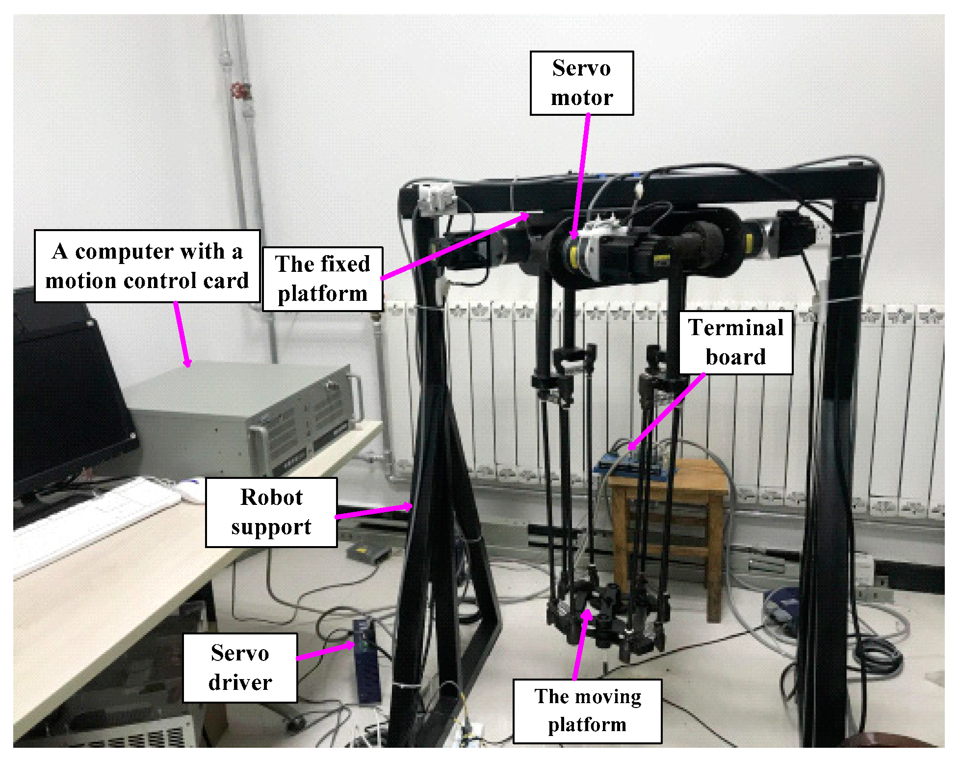
In this section, the planning and optimization methods designed above are verified by some experiments. To compare and analyze the influence of the fifth- and sixth-order polynomial movement rules on mechanical energy consumption, the following scheme was adopted: the basic experiment with a group of data was done first, then the comparison experiments with multiple data were be performed. In the comparison experiments, three parameters, i.e., pick-up span, pick-up height and pick-and-place endpoints coordinates, were taken into consideration. The overall comparative experiments were designed by fixing the values of two parameters and changing the value of the third parameter. In all experiments, the number of wolves was set at 50, and the number of iterations was set at 40. The parameters of the Par4 robot are shown in Table 1, and the experimental platform is shown in Figure 5.

5.1. Basic Experiment

With a group of pick-and-place endpoints taken and the pick-up height given, the trajectory planning above was adopted, i.e., the sleek gate-shaped path based on the Lamé curve was selected, and the fifth- and sixth-order polynomial motion laws were respectively applied to carry out the optimization experiment based on the GWO algorithm for the lowest mechanical energy consumption.
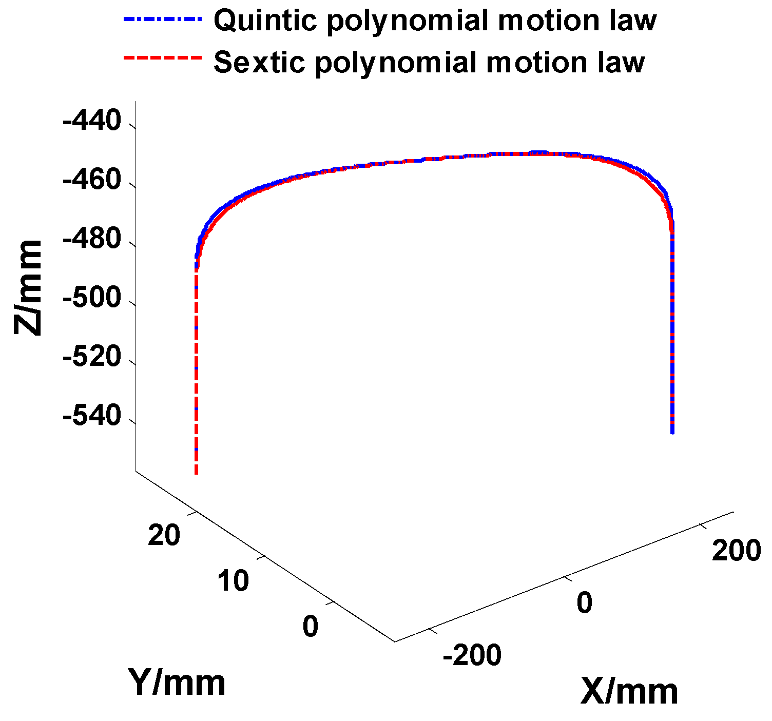
The coordinates of the starting pick-and-place endpoint were set at k 0 = [ 250 , 20 , 543.5 ] , the ending coordinates at k f = [ 250 , 0 , 543.5 ] , and the pick-up height at H a = 100   mm , so then the pick-up span could be obtained as B a = 500.4   mm . The optimal values of parameter e, parameter f, and the minimum mechanical energy consumption (noted as E min for convenience) based on the GWO algorithm are shown in Table 2. The unit of parameters e and f is millimeters (mm), the unit of E min is joules (J). The units of these parameters in subsequent tables are the same. The numerical results in Table 2 reflect the fact that the mechanical energy consumption is relatively smaller under the law of quintic polynomial motion. It is worth mentioning that the optimization result of parameter e is the same (250.2 mm, B a / 2 ) regardless of the motion law of the quintic polynomial or the sextic polynomial. However, the optimization result of Parameter f is not the same. The optimal values in Table 2 were taken, and the trajectory planning method above was implemented. Then, the trajectories were obtained under the fifth-order and sixth-order polynomial motion laws, as shown in Figure 6.
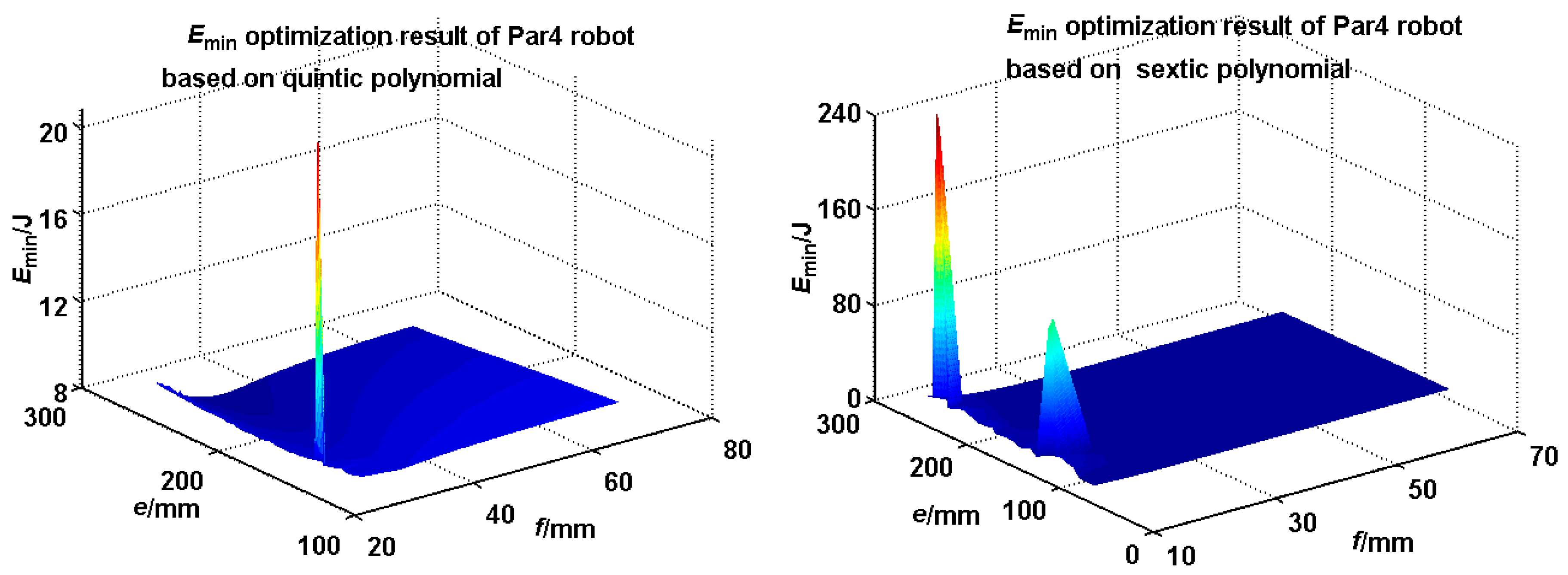
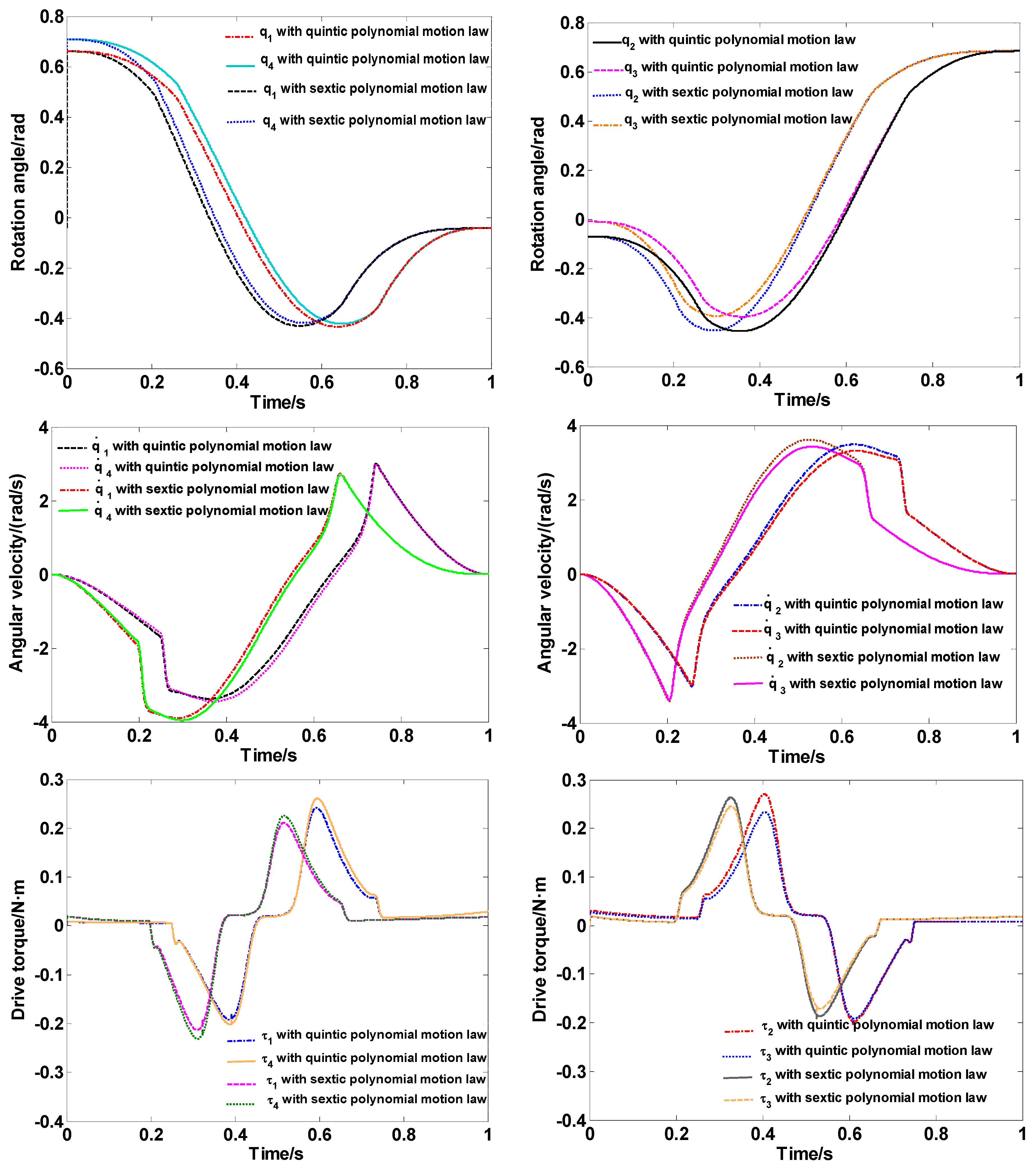
The iteration trajectory of mechanical energy consumption E min is shown in Figure 7. From the results in Figure 7, the overall E min value of the quintic polynomial motion law (left figure) is smaller than that of the sextic polynomial motion law (right figure). When the E min reading is at a higher value, the left graph displays a thin thread-like peak in Figure 7, which shows that only a few wolves in the GWO algorithm failed to find the best prey in time. In other words, in the iterative process, GWO has higher efficiency and faster convergence under the law of quintic polynomial motion. The rotation angles, angular velocities, and corresponding drive torques of each joint of the Par4 parallel robot were obtained based on the optimum parameters e and f, which are shown in Figure 8.

5.2. Experiments with the Same Pick-and-Place Endpoints and Different Pick-Up Heights

Table 3 shows the optimization results with the minimum mechanical energy consumption when the pick-and-place endpoint coordinates were set at k 0 = [ 250 , 20 , 543.5 ] and k f = [ 250 , 0 , 543.5 ] , thus the pick-up span was fixed at B a = 500.4   mm . The pick-up heights were set at 100, 110, 120, 130, 140 and 150 mm, respectively. According to the results in Table 3, the mechanical energy consumption of the sextic polynomial was slightly higher than that of the quintic polynomial. In addition, at different pick-up heights, the optimal value of parameter e was 250.2 mm (this value is B a / 2 ) regardless of the movement law of the quintic or sextic polynomial, and the optimal value of parameter f increases with the increase in pick-up height.

5.3. Experiments with Different Pick-and-Place Endpoints and the Same Pick-Up Height and Span

For the sake of comparison and analysis, here, five groups of different pick-and-place endpoints were taken for planning and comparison in the Par4 robot’s spatial feasible region. The X and Y axis coordinates of the former two groups of pick-and-place endpoints were both small and far away from the boundary of the robot’s feasible region, while the X or Y axis coordinates of the last three groups of pick-and-place endpoints were relatively larger and closer to the boundary of the robot’s feasible region. In the experiments, the pick-up height was the same, set at 120 mm; the pick-up spans were all set at 500.4 mm. Table 4 shows the optimization results based on GWO, and the minimum mechanical energy consumptions are given accordingly. Since all the Z-axis coordinates (−543.5) were the same, for simplicity, only X-axis and Y-axis coordinates are listed in Table 4 for the pick-and-place endpoints.
From Table 4, the mechanical energy consumptions under the former two sets of coordinates were relatively lower than those under the last three sets of coordinates, and in particular, the E min values for the fourth set of coordinates were the highest. Moreover, in the experiments, the mechanical energy consumption based on the quintic polynomial was less than that based on the sextic polynomial under the same conditions. Besides, it is worth mentioning that almost all of the optimal values of parameter e were 250.2 mm (this value is B a / 2 ), while the optimal values of parameter f were relatively smaller in the former two sets of coordinates than those in the last three sets of coordinates, which were close to the pick-up height H a (120 mm). Hence, the optimal value of parameter f is related to the spatial coordinates of the pick-and-place endpoints.

5.4. Experiments with Different Pick-Up Spans, Different Pick-and-Place Endpoints and the Same Pick-Up Height

The pick-up height was taken as 120 mm, and six groups of different pick-and-place endpoints were selected, of which the corresponding pick-up spans are shown in Table 5 as B a / 2 . Since all the Z axis coordinates are −543.5, only X axis and Y axis coordinates of the pick-and-place endpoints are listed in Table 5, for simplicity. In Table 5, the difference between the two motion laws of quintic and sextic polynomials is not obvious when the pick-up height and the pick-and-place coordinates are the same. If the average mechanical energy consumption (denoted as average E min ) in the six different groups of coordinates is taken for comparison, the value under the quintic polynomial motion law is lower than the one under the sextic polynomial motion law. In addition, regardless of the movement law of the quintic or sextic polynomial, almost all the optimization values of parameter e are equal to B a / 2 , but the optimization feature of parameter f is not so obvious, and its value is not only related to the movement law but also related to the pick-and-place endpoints.

6. Conclusions

The main work of this paper is as follows:
1. The Lamé curve was employed in the trajectory planning of the Par4 parallel robot, and the piecewise design method was adopted. Detailed analysis and precise planning were elaborated, focusing on displacement, velocity, and acceleration in the Par4 parallel robot end operating space.
2. To minimize the total mechanical energy consumption of the driving joints, asymmetric displacement planning was introduced based on the quintic and sextic polynomial motion laws. A series of experiments were performed to compare and analyze the mechanical energy consumption of the Par4 parallel robot under the quintic and sextic polynomial motion laws. The results reflect that the mechanical energy consumption is lower when the motion law of the quintic polynomial is adopted.
3. To find the optimal trajectory, the recently proposed GWO algorithm was used. After a series of experiments to minimize the total mechanical energy consumption, it turned out that the optimal value of parameter e of the Lamé curve can be set as half of the pick-up span in the Par4 parallel robot’s trajectory planning, while the optimal value of parameter f depends on different pick-up heights and different pick-and-place endpoints.
In addition, the mechanical energy consumption is related not only to the pick-up height and pick-up span of the trajectory, but also to the coordinate position of the pick-and-place endpoints. The closer the pick-and-place endpoints to the boundary of the Par4 parallel robot’s feasible region, the higher the mechanical energy consumption will be.
The trajectory planning method proposed in this paper is also suitable for other parallel robots, such as Delta parallel robots. Although the trajectory is based on the Lamé curve in this paper, the design method is well suited to two-dimensional curves whose coordinate variables can both be expressed as functions of an intermediate variable that changes over time, such as the circle, the transitional parametric spline curve, and so on.

Author Contributions

Z.M., as the corresponding author, takes primary responsibility for this article. X.Z. drafted the manuscript. All co-authors reviewed the manuscript.

Funding

This research was funded by the National High-Tech Research and Development Program (863 Torch Program) (grant no. 2015AA7041003), the Educational Reform Project of Xianyang Normal University (grant no. 2017Y004), and the Scientific Research Plan Projects of Shaanxi Education Department (grant no. 15JK1784).

Conflicts of Interest

The authors declare no conflict of interest.

References

  1. Song, X.G.; Zhao, Y.J.; Jin, L.; Zhang, P.; Chen, C.W. Dynamic feedforward control in decoupling space for a four-degree-of-freedom parallel robot. Int. J. Adv. Robot. Syst. 2019, 2, 1–10. [Google Scholar] [CrossRef]
  2. Sohn, J.W.; Kim, G.W.; Choi, S.B. A State-of-the-Art Review on Robots and Medical Devices Using Smart Fluids and Shape Memory Alloys. Appl. Sci. 2018, 8, 1928. [Google Scholar] [CrossRef]
  3. Nabat, V.; François, P.; Poignet, P. Dynamic Modeling and Identification of Par4, A Very High Speed Parallel Manipulator. In Proceedings of the IEEE/RSJ International Conference on Intelligent Robots & Systems, Beijing, China, 9–15 October 2006. [Google Scholar]
  4. Staicu, S.; Shao, Z.F.; Zhang, Z.K.; Tang, X.Q.; Wang, L.P. Kinematic analysis of the X4 translational–rotational parallel robot. Int. J. Adv. Robot Syst. 2018, 10, 1–12. [Google Scholar] [CrossRef]
  5. Sun, T.; Liang, D.; Song, Y.M. Singular-Perturbatio-Based Nonlinear Hybrid Control of Redundant Parallel Robot. IEEE T. Ind. Electron. 2018, 65, 3326–3336. [Google Scholar] [CrossRef]
  6. Francisco, G.S.; Jorge, O.S.; Raymundo, J.T.; Ricardo, P.P. A stable proportional–proportional integral tracking controller with self-organizing fuzzy-tuned gains for parallel robots. Int. J. Adv. Robot. Syst. 2019, 2, 1–16. [Google Scholar]
  7. Mohan, S.; Corves, B. Inverse dynamics and trajectory tracking control of a new six degrees of freedom spatial 3-RPRS parallel manipulator. Mech. Sci. 2017, 8, 235–248. [Google Scholar] [CrossRef] [Green Version]
  8. Vincent, R.; Mohammed, T.; Gilles, L. Fast genetic algorithm path planner for fixed-wing military UAV using GPU. IEEE Trans. Aero. Electron. Syst. 2018, 54, 2105–2117. [Google Scholar]
  9. Farajtabar, M.; Daniali, H.M.; Varedi, S.M. Pick and place trajectory planning of planar 3-RRR parallel manipulator in the presence of joint clearance. Robotica 2017, 35, 241–253. [Google Scholar] [CrossRef]
  10. Lin, C.J.; Chen, C.T. Reconfiguration for the Maximum Dynamic Wrench Capability of a Parallel Robot. Appl. Sci. 2016, 6, 80. [Google Scholar] [CrossRef]
  11. Kucuk, S. Optimal trajectory generation algorithm for serial and parallel manipulators. Robot. Cim. Int. Manuf. 2017, 48, 219–232. [Google Scholar] [CrossRef]
  12. Jiang, X.L.; Barnett, E.; Gosselin, C. Dynamic point-to-point trajectory planning beyond the static workspace for six-dof cable-suspended parallel robots. IEEE Trans. Robot. 2018, 34, 781–793. [Google Scholar] [CrossRef]
  13. Jiang, X.L.; Gosselin, C. Dynamic point-to-point trajectory planning of a three-dof cable-suspended parallel robot. IEEE Trans. Robot. 2016, 32, 1550–1557. [Google Scholar] [CrossRef]
  14. Zhang, N.; Shang, W.W.; Cong, S. Geometry-based trajectory planning of a 3-3 cable-suspended parallel robot. IEEE Trans. Robot. 2017, 33, 484–491. [Google Scholar] [CrossRef]
  15. Chen, Y.D.; Li, L. Predictable trajectory planning of industrial robots with constraints. Appl. Sci. 2018, 8, 2648. [Google Scholar] [CrossRef]
  16. Jahanpour, J.; Motallebi, M.; Porghoveh, M. A novel trajectory planning scheme for parallel machining Robots enhanced with NURBS curves. J. Intell. Robot. Syst. 2016, 82, 257–275. [Google Scholar] [CrossRef]
  17. Nan, W.H.; Tang, X.Q.; Song, B. A new automatic motion planning algorithm for a 4-degree-of-freedom parallel kinematic manipulator based on the centre sphere method. Proc. Inst. Mech. Eng. Part B J. Eng. Manuf. 2015, 229, 64–77. [Google Scholar] [CrossRef]
  18. Chen, Z.H.; Wang, Y.; Ouyang, P.; Huang, J.; Zhang, W.J. A novel iteration-based controller for hybrid machine systems for trajectory tracking at the end-effector level. Robotica 2011, 29, 317–324. [Google Scholar] [CrossRef]
  19. Mei, J.P.; Zang, J.W.; Qiao, Z.Y.; Liu, S.T.; Song, T. Trajectory planning of 3-DOF Delta parallel manipulator. J. Mech. Eng. 2016, 52, 9–17. [Google Scholar] [CrossRef]
  20. Bourbonnais, F.; Bigras, P.; Bonev, I.A. Minimum- time trajectory planning and control of a pick-and-place five-bar parallel robot. IEEE/ASME Trans. Mech. 2015, 20, 740–749. [Google Scholar] [CrossRef]
  21. Bonami, P.; Olivares, A.; Staffetti, E. Energy-optimal multi-goal motion planning for planar robot manipulators. J. Optimiz. Theory App. 2014, 163, 80–104. [Google Scholar] [CrossRef]
  22. Petrinec, K.; Kovačić, Z. Trajectory planning algorithm based on the continuity of jerk. In Proceedings of the 15th Mediterranean Conference on Control and Automation, Athens, Greece, 27–29 June 2007. [Google Scholar]
  23. Chen, C.T.; Liao, T.T. Trajectory planning of parallel kinematic manipulators for the maximum dynamic load-carrying capacity. Meccanica 2016, 51, 1653–1674. [Google Scholar] [CrossRef]
  24. Fares, J.A.; Iyad, F.A.; Rasha, M.A.; Mohamed, A. Statistical evaluation of an evolutionary algorithm for minimum time trajectory planning problem for industrial robots. Int. J. Adv. Manuf. Technol. 2017, 89, 389–406. [Google Scholar]
  25. Su, T.T.; Cheng, L.; Wang, Y.K.; Liang, X.; Zheng, J.; Zhang, H.J. Time-optimal trajectory planning for Delta robot based on quintic Pythagorean-hodograph curves. IEEE Access. 2018, 6, 28530–28539. [Google Scholar] [CrossRef]
  26. Abe, A. Minimum energy trajectory planning method for robot manipulator mounted on flexible base. In Proceedings of the 9th Asian Control Conference (ASCC), Istanbul, Turkey, 23–26 June 2013. [Google Scholar]
  27. Sun, Z.H.; Zhang, B.; Cheng, L.; Zhang, W.J. Application of the redundant servomotor approach to design of path generator with dynamic performance improvement. Mech. Mach. Theory 2011, 46, 1784–1795. [Google Scholar] [CrossRef]
  28. Zhang, T.; Zhang, W.J.; Gupta, M.M. An underactuated self-reconfigurable robot and the reconfiguration evolution. Mech. Mach. Theory 2018, 124, 248–258. [Google Scholar] [CrossRef]
  29. Shintaku, E. Minimum energy trajectory for an underwater manipulator and its simple planning method by using a genetic algorithm. Adv. Robot. 1999, 13, 115–138. [Google Scholar] [CrossRef]
  30. Mo, J.; Shao, Z.F.; Guan, L.W.; Xie, F.G. Dynamic performance analysis of the X4 high-speed pick-and-place parallel robot. Robot. Cim. Int. Manuf. 2017, 46, 48–57. [Google Scholar] [CrossRef]
  31. Li, Y.H.; Huang, T.; Chetwynd, D.G. An approach for smooth trajectory planning of high-speed pick-and-place parallel robots using quintic B-splines. Mech. Mach. Theory 2018, 126, 479–490. [Google Scholar] [CrossRef] [Green Version]
  32. Zhang, N.; Shang, W.W.; Cong, S. Dynamic trajectory planning for a spatial 3-DoF cable-suspended parallel robot. Mech. Mach. Theory 2018, 122, 177–196. [Google Scholar] [CrossRef]
  33. Machmudah, A.; Parman, S.; Zainuddin, A.; Chacko, S. Polynomial joint angle arm robot motion planning in complex geometrical obstacles. Appl. Soft. Comput. 2013, 13, 1099–1109. [Google Scholar] [CrossRef]
  34. Barnard, C.J.; Briot, S.; Caro, S. Trajectory generation for high speed pick and place robots. In Proceedings of the ASME 2012 11th Biennial Conference on Engineering Systems Design, Nantes, France, 2–4 July 2012. [Google Scholar]
  35. Six, D.; Briot, S.; Chriette, A.; Martinet, P. The kinematics, dynamics and control of a flying parallel robot with three quadrotors. IEEE Robot. Autom. Lett. 2018, 3, 559–566. [Google Scholar] [CrossRef]
  36. Gauthier, J.F.; Angeles, J.; Nokleby, S. Optimization of a Test Trajectory for Scara Systems; Springer: Berlin/Heidelberg, Germany, 2008. [Google Scholar]
  37. Xie, Z.X.; Li, B.; Ren, P. Energy-Based optimization and experimental validation of the pick-and-place trajectories for the delta parallel robot. Comput. Integr. Manuf. 2018, 24, 3073–3081. [Google Scholar]
  38. Mirjalili, S.; Mirjalili, S.M.; Lewis, A. Grey wolf optimizer. Adv. Eng. Softw. 2014, 69, 46–61. [Google Scholar] [CrossRef]
  39. Zhang, X.Q.; Ming, Z.F. An optimized grey wolf optimizer based on a mutation operator and eliminating-reconstructing mechanism and its application. Front. Inform. Technol. Electron. Eng. 2017, 18, 1705–1719. [Google Scholar] [CrossRef]
  40. Ali, M.E.; Hassan, M.H. Dynamic global maximum power point tracking of the PV systems under variant partial shading using hybrid GWO-FLC. Sol. Energy 2019, 177, 306–316. [Google Scholar]
  41. Rao, A.M.; Ramji, K.; Kumar, T.N. Intelligent navigation of mobile robot using grey wolf colony optimization. Mater. Today Proc. 2018, 5, 19116–19125. [Google Scholar]
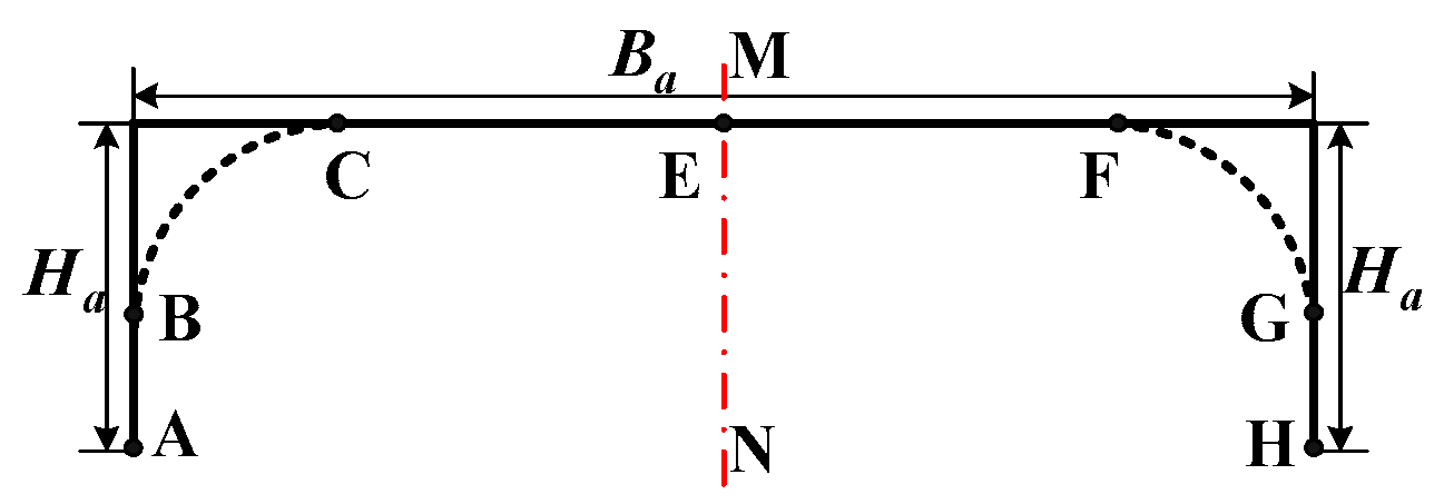
Figure 1. Motion trajectory.
Applsci 09 02770 g001
Figure 2. Structure of the Par4 parallel robot. (a) Par4 parallel robot. (b) Structure sketch of the robot. (c) Top view of the end-effector.
Applsci 09 02770 g002
Figure 3. The half-way motion trajectory.
Applsci 09 02770 g003
Figure 4. The work principle sketch map of the GWO algorithm applied in the trajectory planning.
Applsci 09 02770 g004
Figure 5. The Par4 parallel robot platform.
Applsci 09 02770 g005
Figure 6. Motion trajectory.
Applsci 09 02770 g006
Figure 7. Iterative results of the minimum mechanical energy consumption based on GWO.
Applsci 09 02770 g007
Figure 8. Curves of rotation angle, angular velocity, and drive torque.
Applsci 09 02770 g008
Table 1. Par4 parallel robot-related parameters.
Parameter NameValue
Length of big arm Li273 mm
Length of small arm li600 mm
Radius of big arm revolute R190 mm
Length of moving platform along x axis d160 mm
Length of moving platform along y axis h160 mm
Distance between Bi and Ci along y axis hi20 mm
Distance between Bi and Ci along x axis di20 mm
Load mass of moving platform mc0 kg
Mass of big arm mb0.08 kg
Mass of small arm ms0.07 kg
Mass of moving platform md2.6 kg
Mass of big arm end connections mend0.59 kg
Table 2. Results of parameter optimization based on GWO.
Motion Lawe/mmf/mm E min / J
Quintic polynomial250.232.38.209
Sextic polynomial250.238.28.500
Table 3. Optimized results with different H a , the same B a and the same endpoints.
Motion   Law / H a Quintic PolynomialSextic Polynomial
e/mmf/mm E min / J e/mmf/mm E min / J
100 mm250.232.38.209250.238.28.500
110 mm250.233.78.757250.240.29.054
120 mm250.235.49.323250.242.39.628
130 mm250.237.19.912250.244.610.224
140 mm250.238.710.528250.247.110.847
150 mm250.240.511.178250.250.011.503
Table 4. Optimized results with the same H a , the same B a and different endpoints.
Motion Law/Pick-and-Place PointsQuintic PolynomialSextic Polynomial
k 0 k f e/mmf/mm E min / J e/mmf/mm E min / J
[−200,237.6][150,−120]250.239.29.445250.250.39.566
[−250,20][250,0]250.235.49.323250.242.39.628
[20,20][360,387.2]250.2120.011.266250.212012.515
[−10,−20][−260,−453.5]250.2120.015.142250.012015.167
[0,200][−400,−100.7]250.2120.010.954250.212010.963
Table 5. Optimized results with the same H a , different B a and different endpoints.
Motion Law/Pick-and-Place Points Quintic PolynomialSextic Polynomial
k 0 k f Ba/2/mme/mmf/mm E min / J e/mmf/mm E min / J
[80,30][30,−20]35.435.481.57.28335.376.87.287
[75,55][−35,150]72.772.71207.74672.71207.744
[150,50][−50,20]101.1101.11207.883101.11207.878
[300,0][−10,75]159.5159.5120.07.721159.51207.711
[−210,50][150,235]202.4202.437.08.852202.440.88.890
[0,−305][0,396.7]350.9350.963.311.048350.976.511.124
average E min 8.422 8.439