Estimating the Heating Load of Buildings for Smart City Planning Using a Novel Artificial Intelligence Technique PSO-XGBoost


Abstract
1. Introduction
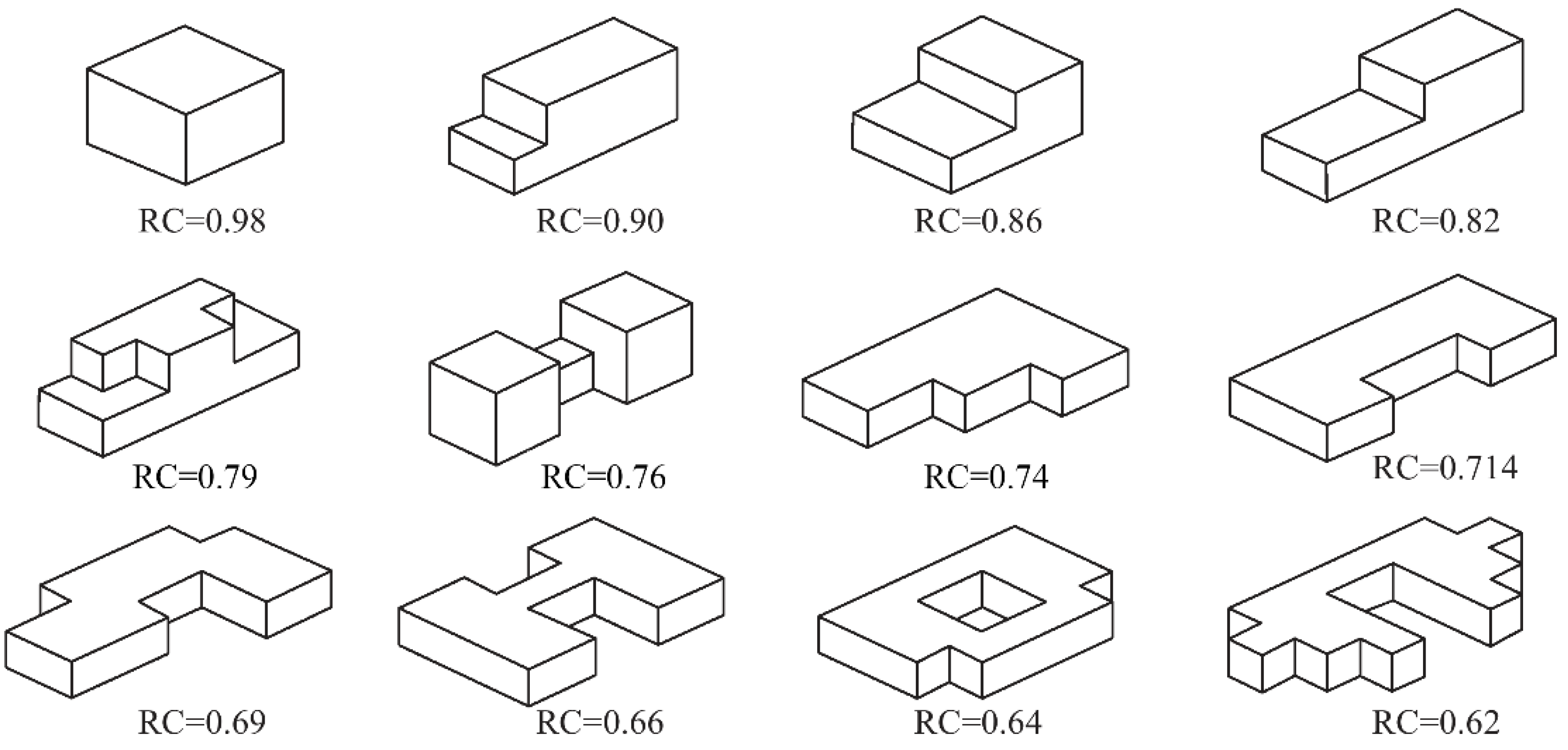
2. Experimental Database
3. Background of the Methods Used
3.1. Particle Swarm Optimization (PSO) Algorithm
3.2. Extreme Gradient Boosting Machine (XGBoost)
3.3. Support Vector Machine (SVM)
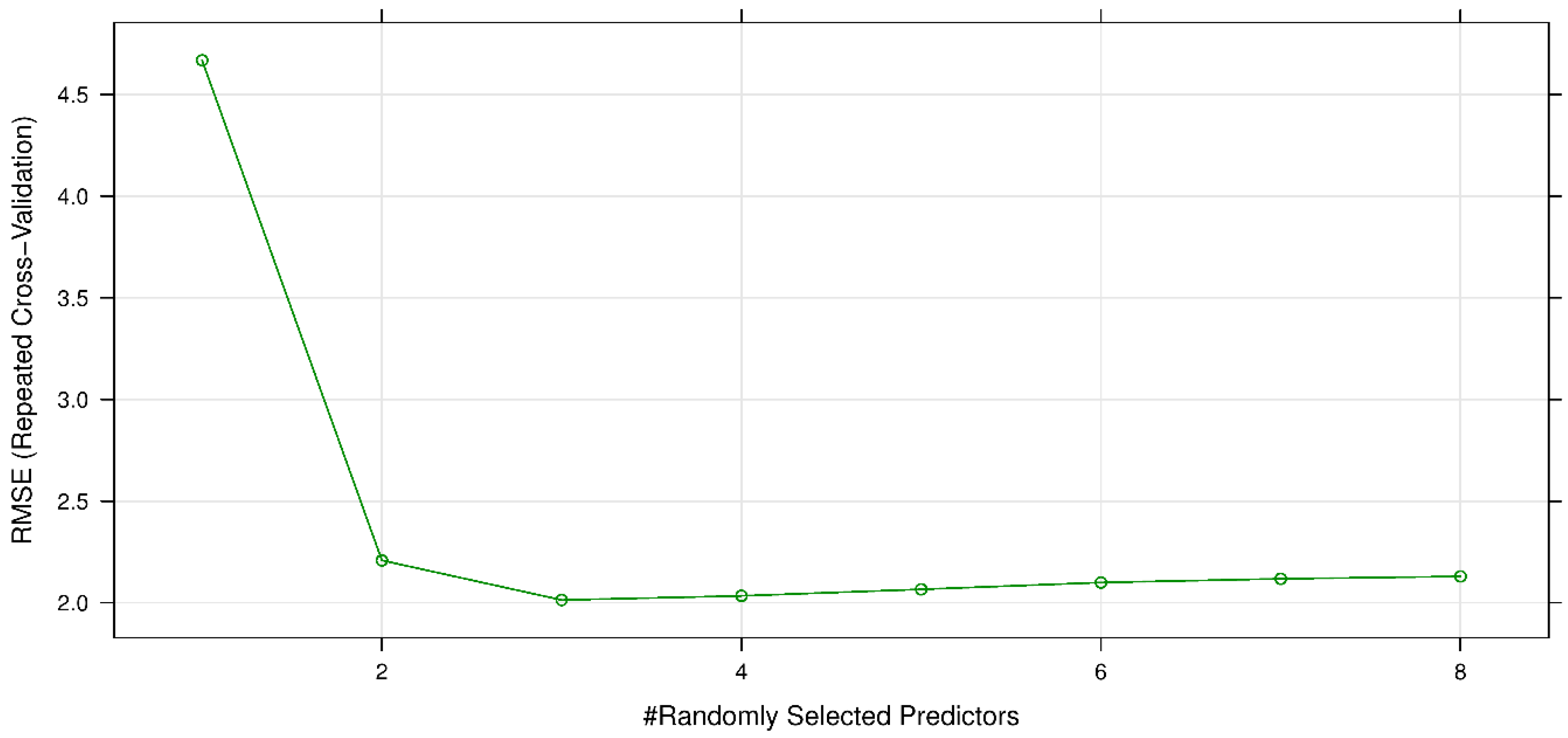
3.4. Random Forest (RF)
3.5. Gaussian Process (GP)
3.6. Classification and Regression Tree (CART)
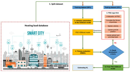
4. Proposing the PSO-XGBoost Framework for Estimating HL
5. Performance Evaluation Indices
6. Results and Discussions
7. Conclusions and Remarks
Author Contributions
Funding
Acknowledgments
Conflicts of Interest
References
- Lin, Y.-H. Design and Implementation of an IoT-Oriented Energy Management System Based on Non-Intrusive and Self-Organizing Neuro-Fuzzy Classification as an Electrical Energy Audit in Smart Homes. Appl. Sci. 2018, 8, 2337. [Google Scholar] [CrossRef]
- De Paz, J.F.; Bajo, J.; Rodríguez, S.; Villarrubia, G.; Corchado, J.M. Intelligent system for lighting control in smart cities. Inf. Sci. 2016, 372, 241–255. [Google Scholar] [CrossRef]
- Hao, L.; Lei, X.; Yan, Z.; ChunLi, Y. The application and implementation research of smart city in China. In Proceedings of the 2012 International Conference on System Science and Engineering (ICSSE), Dalian, China, 30 June–2 July 2012; pp. 288–292. [Google Scholar]
- Alsarraf, J.; Moayedi, H.; Rashid, A.S.A.; Muazu, M.A.; Shahsavar, A. Application of PSO–ANN modelling for predicting the exergetic performance of a building integrated photovoltaic/thermal system. Eng. Comput. 2019. [Google Scholar] [CrossRef]
- Wang, D.; Pang, X.; Wang, W.; Qi, Z.; Li, J.; Luo, D. Assessment of the Potential of High-Performance Buildings to Achieve Zero Energy: A Case Study. Appl. Sci. 2019, 9, 775. [Google Scholar] [CrossRef]
- Olszewski, R.; Pałka, P.; Turek, A.; Kietlińska, B.; Płatkowski, T.; Borkowski, M. Spatiotemporal Modeling of the Smart City Residents’ Activity with Multi-Agent Systems. Appl. Sci. 2019, 9, 2059. [Google Scholar] [CrossRef]
- Yu, Z.; Haghighat, F.; Fung, B.C.; Yoshino, H. A decision tree method for building energy demand modeling. Energy Build. 2010, 42, 1637–1646. [Google Scholar] [CrossRef]
- Zhao, H.-X.; Magoulès, F. A review on the prediction of building energy consumption. Renew. Sustain. Energy Rev. 2012, 16, 3586–3592. [Google Scholar] [CrossRef]
- Aparicio-Ruiz, P.; Guadix-Martín, J.; Barbadilla-Martín, E.; Muñuzuri-Sanz, J. Applying Renewable Energy Technologies in an Integrated Optimization Method for Residential Building’s Design. Appl. Sci. 2019, 9, 453. [Google Scholar] [CrossRef]
- De Boeck, L.; Verbeke, S.; Audenaert, A.; De Mesmaeker, L. Improving the energy performance of residential buildings: A literature review. Renew. Sustain. Energy Rev. 2015, 52, 960–975. [Google Scholar] [CrossRef]
- Eskin, N.; Türkmen, H. Analysis of annual heating and cooling energy requirements for office buildings in different climates in Turkey. Energy Build. 2008, 40, 763–773. [Google Scholar] [CrossRef]
- Nojavan, S.; Majidi, M.; Zare, K. Optimal scheduling of heating and power hubs under economic and environment issues in the presence of peak load management. Energy Convers. Manag. 2018, 156, 34–44. [Google Scholar] [CrossRef]
- Yang, I.-H.; Yeo, M.-S.; Kim, K.-W. Application of artificial neural network to predict the optimal start time for heating system in building. Energy Convers. Manag. 2003, 44, 2791–2809. [Google Scholar] [CrossRef]
- Braun, M.; Altan, H.; Beck, S. Using regression analysis to predict the future energy consumption of a supermarket in the UK. Appl. Energy 2014, 130, 305–313. [Google Scholar] [CrossRef]
- Jovanović, R.Ž.; Sretenović, A.A.; Živković, B.D. Ensemble of various neural networks for prediction of heating energy consumption. Energy Build. 2015, 94, 189–199. [Google Scholar] [CrossRef]
- Sholahudin, S.; Han, H. Simplified dynamic neural network model to predict heating load of a building using Taguchi method. Energy 2016, 115, 1672–1678. [Google Scholar] [CrossRef]
- Gunay, B.; Shen, W.; Newsham, G. Inverse blackbox modeling of the heating and cooling load in office buildings. Energy Build. 2017, 142, 200–210. [Google Scholar] [CrossRef]
- Ahmad, T.; Chen, H. Short and medium-term forecasting of cooling and heating load demand in building environment with data-mining based approaches. Energy Build. 2018, 166, 460–476. [Google Scholar] [CrossRef]
- Kim, E.-J.; He, X.; Roux, J.-J.; Johannes, K.; Kuznik, F. Fast and accurate district heating and cooling energy demand and load calculations using reduced-order modelling. Appl. Energy 2019, 238, 963–971. [Google Scholar] [CrossRef]
- Bui, X.-N.; Moayedi, H.; Rashid, A.S.A. Developing a predictive method based on optimized M5Rules–GA predicting heating load of an energy-efficient building system. Eng. Comput. 2019, 1–10. [Google Scholar] [CrossRef]
- Jitkongchuen, D.; Pacharawongsakda, E. Prediction Heating and Cooling Loads of Building Using Evolutionary Grey Wolf Algorithms. In Proceedings of the 2019 Joint International Conference on Digital Arts, Media and Technology with ECTI Northern Section Conference on Electrical, Electronics, Computer and Telecommunications Engineering (ECTI DAMT-NCON), Nan, Thailand, 30 January–2 February 2019; pp. 93–97. [Google Scholar]
- Al-Shammari, E.T.; Keivani, A.; Shamshirband, S.; Mostafaeipour, A.; Yee, L.; Petković, D.; Ch, S. Prediction of heat load in district heating systems by Support Vector Machine with Firefly searching algorithm. Energy 2016, 95, 266–273. [Google Scholar] [CrossRef]
- Sajjadi, S.; Shamshirband, S.; Alizamir, M.; Yee, L.; Mansor, Z.; Manaf, A.A.; Altameem, T.A.; Mostafaeipour, A. Extreme learning machine for prediction of heat load in district heating systems. Energy Build. 2016, 122, 222–227. [Google Scholar] [CrossRef]
- Pino-Mejías, R.; Pérez-Fargallo, A.; Rubio-Bellido, C.; Pulido-Arcas, J.A. Comparison of linear regression and artificial neural networks models to predict heating and cooling energy demand, energy consumption and CO2 emissions. Energy 2017, 118, 24–36. [Google Scholar] [CrossRef]
- Xie, L. The heat load prediction model based on BP neural network-markov model. Procedia Comput. Sci. 2017, 107, 296–300. [Google Scholar] [CrossRef]
- Protić, M.; Shamshirband, S.; Anisi, M.H.; Petković, D.; Mitić, D.; Raos, M.; Arif, M.; Alam, K.A. Appraisal of soft computing methods for short term consumers’ heat load prediction in district heating systems. Energy 2015, 82, 697–704. [Google Scholar] [CrossRef]
- Mottahedi, M.; Mohammadpour, A.; Amiri, S.S.; Riley, D.; Asadi, S. Multi-linear regression models to predict the annual energy consumption of an office building with different shapes. Procedia Eng. 2015, 118, 622–629. [Google Scholar] [CrossRef]
- Kim, W.; Kim, Y.-K. Optimal Operation Methods of the Seasonal Solar Borehole Thermal Energy Storage System for Heating of a Greenhouse. J. Korea Acad.-Ind. Coop. Soc. 2019, 20, 28–34. [Google Scholar]
- Wang, Z.; Srinivasan, R.S. A review of artificial intelligence based building energy use prediction: Contrasting the capabilities of single and ensemble prediction models. Renew. Sustain. Energy Rev. 2017, 75, 796–808. [Google Scholar] [CrossRef]
- Tsanas, A.; Xifara, A. Accurate quantitative estimation of energy performance of residential buildings using statistical machine learning tools. Energy Build. 2012, 49, 560–567. [Google Scholar] [CrossRef]
- TCVN. Solid minerals fuels—Determination of ash. 1995, 173. [Google Scholar]
- Pessenlehner, W.; Mahdavi, A. Building Morphology, Transparence, and Energy Performance; Eighth international IBPSA conference: Eindhoven, Netherlands, 2003. [Google Scholar]
- Schiavon, S.; Lee, K.H.; Bauman, F.; Webster, T. Influence of raised floor on zone design cooling load in commercial buildings. Energy Build. 2010, 42, 1182–1191. [Google Scholar] [CrossRef]
- Nguyen, H. Support vector regression approach with different kernel functions for predicting blast-induced ground vibration: A case study in an open-pit coal mine of Vietnam. SN Appl. Sci. 2019, 1, 283. [Google Scholar] [CrossRef]
- Bui, X.N.; Nguyen, H.; Le, H.A.; Bui, H.B.; Do, N.H. Prediction of Blast-induced Air Over-pressure in Open-Pit Mine: Assessment of Different Artificial Intelligence Techniques. Nat. Resour. Res. 2019. [Google Scholar] [CrossRef]
- Hasanipanah, M.; Faradonbeh, R.S.; Amnieh, H.B.; Armaghani, D.J.; Monjezi, M. Forecasting blast-induced ground vibration developing a CART model. Eng. Comput. 2017, 33, 307–316. [Google Scholar] [CrossRef]
- Rasmussen, C.E. Gaussian processes in machine learning. In Summer School on Machine Learning; Springer: Berlin/Heidelberg, Germany, 2003; pp. 63–71. [Google Scholar]
- Grange, S.K.; Carslaw, D.C.; Lewis, A.C.; Boleti, E.; Hueglin, C. Random forest meteorological normalisation models for Swiss PM 10 trend analysis. Atmos. Chem. Phys. 2018, 18, 6223–6239. [Google Scholar] [CrossRef]
- Moayedi, H.; Hayati, S. Modelling and optimization of ultimate bearing capacity of strip footing near a slope by soft computing methods. Appl. Soft Comput. 2018, 66, 208–219. [Google Scholar] [CrossRef]
- Nguyen, H.; Drebenstedt, C.; Bui, X.-N.; Bui, D.T. Prediction of Blast-Induced Ground Vibration in an Open-Pit Mine by a Novel Hybrid Model Based on Clustering and Artificial Neural Network. Nat. Resour. Res. 2019. [Google Scholar] [CrossRef]
- Nguyen, H.; Bui, X.-N.; Tran, Q.-H.; Mai, N.-L. A new soft computing model for estimating and controlling blast-produced ground vibration based on hierarchical K-means clustering and cubist algorithms. Appl. Soft Comput. 2019, 77, 376–386. [Google Scholar] [CrossRef]
- Nguyen, H.; Bui, X.-N.; Moayedi, H. A comparison of advanced computational models and experimental techniques in predicting blast-induced ground vibration in open-pit coal mine. Acta Geophys. 2019. [Google Scholar] [CrossRef]
- Eberhart, R.; Kennedy, J. A new optimizer using particle swarm theory. In Proceedings of the Sixth International Symposium on Micro Machine and Human Science, Nagoya, Japan, 4–6 October 1995; pp. 39–43. [Google Scholar]
- Nguyen, H.; Moayedi, H.; Foong, L.K.; Al Najjar, H.A.H.; Jusoh, W.A.W.; Rashid, A.S.A.; Jamali, J. Optimizing ANN models with PSO for predicting short building seismic response. Eng. Comput. 2019. [Google Scholar] [CrossRef]
- Armaghani, D.J.; Hajihassani, M.; Mohamad, E.T.; Marto, A.; Noorani, S.A. Blasting-induced flyrock and ground vibration prediction through an expert artificial neural network based on particle swarm optimization. Arab. J. Geosci. 2014, 7, 5383–5396. [Google Scholar] [CrossRef]
- Gordan, B.; Armaghani, D.J.; Hajihassani, M.; Monjezi, M. Prediction of seismic slope stability through combination of particle swarm optimization and neural network. Eng. Comput. 2016, 32, 85–97. [Google Scholar] [CrossRef]
- Yang, X.; Zhang, Y.; Yang, Y.; Lv, W. Deterministic and Probabilistic Wind Power Forecasting Based on Bi-Level Convolutional Neural Network and Particle Swarm Optimization. Appl. Sci. 2019, 9, 1794. [Google Scholar] [CrossRef]
- Moayedi, H.; Mehrabi, M.; Mosallanezhad, M.; Rashid, A.S.A.; Pradhan, B. Modification of landslide susceptibility mapping using optimized PSO-ANN technique. Eng. Comput. 2018, 35, 967–984. [Google Scholar] [CrossRef]
- Moayedi, H.; Moatamediyan, A.; Nguyen, H.; Bui, X.-N.; Bui, D.T.; Rashid, A.S.A. Prediction of ultimate bearing capacity through various novel evolutionary and neural network models. Eng. Comput. 2019. [Google Scholar] [CrossRef]
- Kulkarni, R.V.; Venayagamoorthy, G.K. An estimation of distribution improved particle swarm optimization algorithm. In Proceedings of the 2007 3rd International Conference on Intelligent Sensors, Sensor Networks and Information, Melbourne, QLD, Australia, 3–6 December 2007; pp. 539–544. [Google Scholar]
- Friedman, J.H. Stochastic gradient boosting. Comput. Stat. Data Anal. 2002, 38, 367–378. [Google Scholar] [CrossRef]
- Zhou, J.; Li, E.; Wang, M.; Chen, X.; Shi, X.; Jiang, L. Feasibility of Stochastic Gradient Boosting Approach for Evaluating Seismic Liquefaction Potential Based on SPT and CPT Case Histories. J. Perform. Constr. Facil. 2019, 33, 04019024. [Google Scholar] [CrossRef]
- Chen, T.; He, T. Xgboost: Extreme Gradient Boosting; R Package Version 0.4-2; Available online: https://cran.r-project.org/web/packages/xgboost/vignettes/xgboost.pdf (accessed on 11 March 2019).
- Nguyen, H.; Bui, X.-N.; Bui, H.-B.; Cuong, D.T. Developing an XGBoost model to predict blast-induced peak particle velocity in an open-pit mine: A case study. Acta Geophys. 2019, 67, 477–490. [Google Scholar] [CrossRef]
- Cortes, C.; Vapnik, V. Support vector machine. Mach. Learn. 1995, 20, 273–297. [Google Scholar] [CrossRef]
- Dou, J.; Paudel, U.; Oguchi, T.; Uchiyama, S.; Hayakavva, Y.S. Shallow and Deep-Seated Landslide Differentiation Using Support Vector Machines: A Case Study of the Chuetsu Area, Japan. Terr. Atmos. Ocean. Sci. 2015, 26, 227–239. [Google Scholar] [CrossRef]
- Zhou, J.; Li, X.; Shi, X. Long-term prediction model of rockburst in underground openings using heuristic algorithms and support vector machines. Saf. Sci. 2012, 50, 629–644. [Google Scholar] [CrossRef]
- Breiman, L. Random forests. Mach. Learn. 2001, 45, 5–32. [Google Scholar] [CrossRef]
- Effron, B.; Tibshirani, R.J. An introduction to the bootstrap. Monogr. Stat. Appl. Probab. 1993, 57, 436. [Google Scholar]
- Breiman, L. Random Forests; Technical report 567; University of California-Berkeley, Statistic Department, 1999. [Google Scholar]
- Zhou, J.; Shi, X.; Du, K.; Qiu, X.; Li, X.; Mitri, H.S. Feasibility of random-forest approach for prediction of ground settlements induced by the construction of a shield-driven tunnel. Int. J. Geomech. 2016, 17, 04016129. [Google Scholar] [CrossRef]
- Rasmussen, C.E. Gaussian processes in machine learning. In Advanced Lectures on Machine Learning; Springer: Berlin, Germany, 2004; pp. 63–71. [Google Scholar]
- Särkkä, S.; Álvarez, M.A.; Lawrence, N.D. Gaussian Process Latent Force Models for Learning and Stochastic Control of Physical Systems. arXiv 2017, arXiv:1709.05409. [Google Scholar]
- Khandelwal, M.; Armaghani, D.J.; Faradonbeh, R.S.; Yellishetty, M.; Majid, M.Z.A.; Monjezi, M. Classification and regression tree technique in estimating peak particle velocity caused by blasting. Eng. Comput. 2017, 33, 45–53. [Google Scholar] [CrossRef]
- Myles, A.J.; Feudale, R.N.; Liu, Y.; Woody, N.A.; Brown, S.D. An introduction to decision tree modeling. J. Chemom. 2004, 18, 275–285. [Google Scholar] [CrossRef]
- Pradhan, B. A comparative study on the predictive ability of the decision tree, support vector machine and neuro-fuzzy models in landslide susceptibility mapping using GIS. Comput. Geosci. 2013, 51, 350–365. [Google Scholar] [CrossRef]
- Nguyen, H.; Bui, X.-N. Predicting Blast-Induced Air Overpressure: A Robust Artificial Intelligence System Based on Artificial Neural Networks and Random Forest. Nat. Resour. Res. 2018. [Google Scholar] [CrossRef]
- Borgonovo, E. A new uncertainty importance measure. Reliab. Eng. Syst. Saf. 2007, 92, 771–784. [Google Scholar] [CrossRef]
- Da Veiga, S. Global sensitivity analysis with dependence measures. J. Stat. Comput. Simul. 2015, 85, 1283–1305. [Google Scholar] [CrossRef]
- Krzykacz-Hausmann, B. Epistemic sensitivity analysis based on the concept of entropy. In Proceedings of the Sensitivity Analysis of Model Output, Madrid, Spain, 18–20 June 2001; pp. 31–35. [Google Scholar]


| Kernel Functions | Type |
|---|---|
| Linear kernel | |
| Polynomial kernel | |
| Radial primary kernel function | |
| Two-layer neural kernel |
| Parameters | Acronym | Value |
|---|---|---|
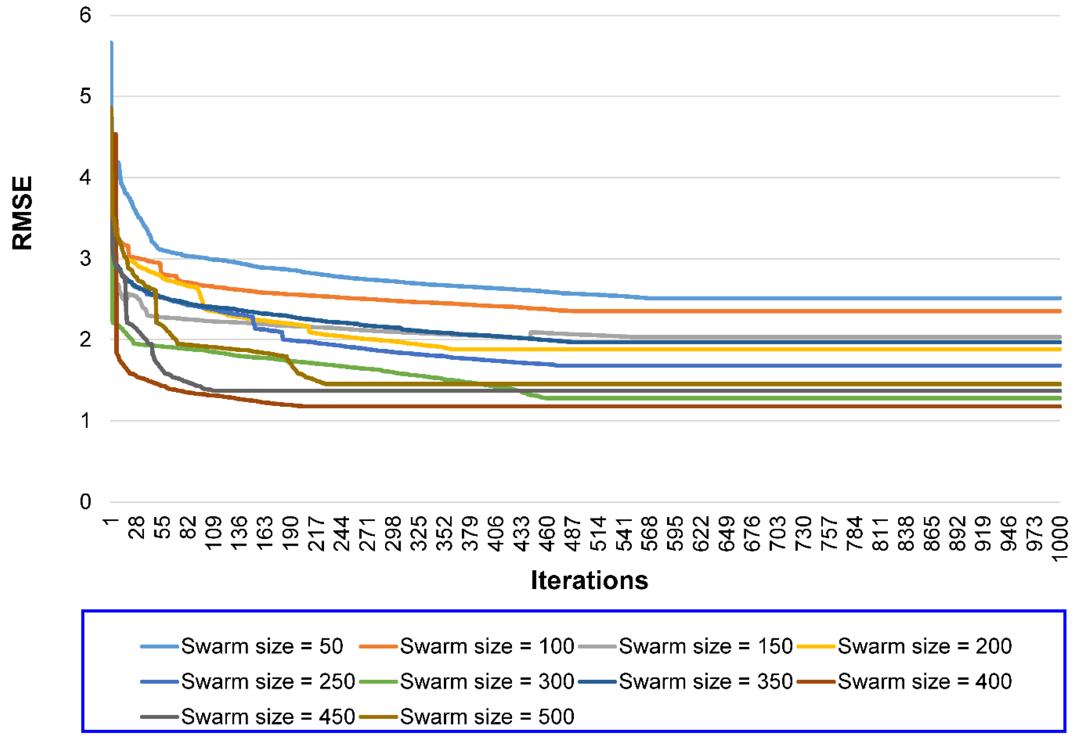
| The number population | p | 50,100,150,200,250,300,350,400,450,500 |
| Maximum particle’s velocity | Vmax | 2.00 |
| Individual cognitive | 1.8 | |
| Group cognitive | 1.8 | |
| Inertia weight | w | 0.95 |
| Maximum number of iteration | mi | 1000 |
| Technique | RMSE | R2 | MAE | VAF | MAPE | Rank for RMSE | Rank for R2 | Rank for MAE | Rank for VAF | Rank for MAPE | Total Ranking |
|---|---|---|---|---|---|---|---|---|---|---|---|
| PSO-XGBoost | 1.124 | 0.990 | 0.615 | 98.934 | 0.024 | 6 | 6 | 5 | 6 | 6 | 29 |
| XGBoost | 1.651 | 0.977 | 0.720 | 97.664 | 0.028 | 3 | 3 | 4 | 3 | 4 | 17 |
| SVM | 1.776 | 0.973 | 0.910 | 97.315 | 0.037 | 2 | 1 | 1 | 2 | 1 | 7 |
| RF | 1.589 | 0.978 | 0.557 | 97.835 | 0.026 | 5 | 4 | 6 | 5 | 5 | 25 |
| GP | 1.632 | 0.978 | 0.798 | 97.726 | 0.033 | 4 | 4 | 2 | 4 | 2 | 16 |
| CART | 1.779 | 0.973 | 0.773 | 97.286 | 0.031 | 1 | 1 | 3 | 1 | 3 | 9 |
© 2019 by the authors. Licensee MDPI, Basel, Switzerland. This article is an open access article distributed under the terms and conditions of the Creative Commons Attribution (CC BY) license (http://creativecommons.org/licenses/by/4.0/).
Share and Cite
Le, L.T.; Nguyen, H.; Zhou, J.; Dou, J.; Moayedi, H. Estimating the Heating Load of Buildings for Smart City Planning Using a Novel Artificial Intelligence Technique PSO-XGBoost. Appl. Sci. 2019, 9, 2714. https://doi.org/10.3390/app9132714
Le LT, Nguyen H, Zhou J, Dou J, Moayedi H. Estimating the Heating Load of Buildings for Smart City Planning Using a Novel Artificial Intelligence Technique PSO-XGBoost. Applied Sciences. 2019; 9(13):2714. https://doi.org/10.3390/app9132714
Chicago/Turabian StyleLe, Le Thi, Hoang Nguyen, Jian Zhou, Jie Dou, and Hossein Moayedi. 2019. "Estimating the Heating Load of Buildings for Smart City Planning Using a Novel Artificial Intelligence Technique PSO-XGBoost" Applied Sciences 9, no. 13: 2714. https://doi.org/10.3390/app9132714
APA StyleLe, L. T., Nguyen, H., Zhou, J., Dou, J., & Moayedi, H. (2019). Estimating the Heating Load of Buildings for Smart City Planning Using a Novel Artificial Intelligence Technique PSO-XGBoost. Applied Sciences, 9(13), 2714. https://doi.org/10.3390/app9132714