A Model-Based Approach of Foreground Region of Interest Detection for Video Codecs

Abstract

Detecting the Region of Interest (ROI) for video clips is a significant and useful technique both in video codecs and surveillance/monitor systems. In this paper, a new model-based detection method is designed which suits video compression codecs by proposing two models: an “inter” and “intra” model. The “inter” model exploits the motion information represented as blocks by global motion compensation approaches while the “intra” model extracts the objects details through objects filtering and image segmentation procedures. Finally, the detection results are formed through a new clustering with fine-tune approach from the “intra” model assisted with the “inter” model. Experimental results show that the proposed method fits well for real-time video codecs and it achieves a good performance both on detection precision and on computing time. In addition, the proposed method is versatile for a wide range of surveillance videos with different characteristics.

1. Introduction

Detecting Region Of Interest (ROI) for video sequences is widely applied both in surveillance/monitor systems and in video encoders. In recent decades, people attempt to define the concept of ROI based on Human Visual System [1]. Also, an ROI-based video encoding mode is adopted both in previous research [2,3] and in latest video codecs such as VPX [4] or HEVC [5]. The notion of ROI is within an evolutionary process, In earlier works [6,7], researchers treat faces as ROI details and adjust quantization parameters (QP) in video compression for ROI encoded blocks. Other works such as [8,9] regard moving or high contrast image segments as ROI details for video codecs. As the concept of the “objected-based” video coding raised from MPEG-4 [10], researchers begin to focus on moving objects extraction and encoding. Hence, ROI is defined more likely as the foreground moving objects in video clips. During the recent five years, many fore-background separation methods are developed based on moving objects detection. The low-rank decomposition method is able to solve the change detection problem by outlier pursuit algorithm, in which the changing components are stored in a sparse matrix. Principle Component Analysis (PCA) has been proposed as a state-of-the-art method for low-rank matrix recovery [11]. However, the classical PCA can be easily corrupted by noise. With the rapid development of artificial intelligence, objects discovery is also used in navigation system designs for autonomous cars, in which computers would recognize objects and make the planning without specialized sensors [12]. Therefore, it is essential to design a detection algorithm for both accuracy and efficiency, so that typical objects in videos or images can be automatically discovered real time to help the computer understand their contents. In addition, object detection can be embedded into the scope of motion estimation (ME) for video coding architectures in our previous works [13,14,15]. Specifically, the detection method based on ME can be embedded into some ME processors. For example, the custom-instruction with the combination of synchronous dynamic random access memory (SDRAM) and on-chip memory architecture-based Nios II processor [16,17], and the FPGA architecture-based processor [18].

1.1. Related Work

One of the state-of-the-art methods for ROI detection is the Gaussian Mixture Model (GMM) [19,20,21], in which fore-background are modeled with some weighted mixture components. Another typical method is named as sparse and low-rank decomposition [11], in which moving objects are computed as the sparse matrix. Derived from this idea, principle component analysis (PCA) [22] is used to efficiently exploit the low-rank structure within errors or outliers, and it is well extended by RPCA [23,24,25] where the robustness is improved to work even in the presence of large errors. Also, a probabilistic model for RPCA is proposed in [26] which provides a good visual results. Other low-rank models are treated as the variations of RPCA such as Grouse [27], RASL [28] and SSGodec [29], in which the computing costs are optimized. Moreover, texture-based objects extraction is proposed in Chan et al. [30,31,32,33]. In these works, the authors cluster and extract dynamic textures by the HEM-DTM approach corresponding with Hidden Markov Model (HMM). In addition, background modeling-based approaches such as Vibe [34], LBP [35], SOBS [36], etc. have introduced different background-model update policies based on time, color-distance, and some reliable factors. Meanwhile, the machine learning approaches such as unsupervised clustering [37,38], Markov Random Field (MRF) for graph cut [39,40,41,42] also achieve a good performance on ROI extraction and detection.

The other parts of research for ROI detection methods focus on deep-learning based method. Architectures of deep neural network with repeated convolution and pooling layers have become the dominant idea for high-quality objects recognition and detection [43]. Szegedy et al. [44] introduced the idea of bounding box masks regression for object detection. Similar works on MultiBox [45,46], improved the previous work by enhancing efficiency and scalability. Ren et al. [47] improved the architecture of R-CNN by proposing a Region Propsal Network (RPN) that shares full-image convolutional features with the detection network. He et al. [48] designed a framework of Spatial Pyramid Pooling (SPP) which enhances robustness to size variations in the network. The paper also claimed that the detection speed was improved compared to R-CNN. YOLO by Redmon et al. [49] used a single network to predict bounding boxes and class labels for objects. Hence, the detection speed has a significant breakthrough. Later, Single Shot Multibox Detector (SSD) [50] by Liu et al. discretized the output space of bounding boxes into a set of default boxes over different resolutions per feature map location. Both the detection speed and the accuracy have been improved since it only uses a single deep neural network with multiple resolutions of feature maps for boxes regression. Other R-CNN based methods [51,52,53] attempted to optimize the network structure by introducing dense connections, reusing computations, applying per-region subnetwork structures to improve the detection performance. However, the multi-stage pipeline training framework of R-CNN brings expensive training costs in space and time. Meanwhile, features extracted from each object proposal are slow at test time [54]. As for machine learning-based methods, a state-of-the-art motivation is to detect objects by using pattern mining with a dictionary model [55]. Our previous work [56] proposed a word-topic model based on Latent Dirichlet Allocation (LDA) model, in which the image features are transformed into corresponding words for ROI object description. Also, an Anchor-box fine-tuning algorithm is proposed to improve the detection precision. It makes a trade-off between the computing costs and model accuracy.

1.2. Overview and Contributions

According to the related research listed, a motivation is to propose a method which suits video codecs like HEVC/VPX. In this paper, a new ROI modeling-based detection scheme is designed which copes with video compression standards by proposing two ROI models: “inter” and “intra”. The “inter” part includes camera status detection and global motion compensation (GMC). The “intra” part includes image segmentation and objects filtering. At last, the detection results are combined together based on the output of two models. Please note that each model can only observe a partial information: The “inter” corresponds with motion information and the “intra” with objects information, as depicted in Figure 1. Previous works [57,58,59,60] introduce an adaptive feature-based methods (FBMs) which estimates the camera motion with error-least matching points assisted by the Single Homographic (SH) matrix. However, minimizing the movement errors of matching points brings computational costs that reduce the speed in real-time systems. To overcome this disadvantage, we propose a fast and approximate global motion compensation way which uses a flexible sampling set and a decision tree model for classification in the “inter” model. The motion vector blocks for objects are acquired via global motion compensation techniques. As for the “intra” model, a Kernel Fuzzy-C Means image segmentation approach is proposed to cluster pixels into specific groups. Then, we use a new motion area pruning method to eliminate the “noise” motion blocks extracted through the “inter” model. Please note that the purpose of “intra” model is to cluster objects by colorspaces and combine them with the motion information separately owing to the connectivity correlation of each cluster.

The contributions of this paper are illustrated below: First, we address the ROI detection problem by designing the “inter” and “intra” models. In the inter model, we first propose a sampling criteria which accurately samples the background motion blocks. Then, a fast and approximate way for global motion detection and compensation techniques based on the camera status and the decision tree model are proposed. In the intra model, a new adaptive and accurate image segmentation method is designed for clustering foreground objects. We innovate combining two models as the finial detection results by developing a combination algorithm based on color correlation and distance. A motion area pruning algorithm is proposed to eliminate noise motion blocks extracted via GMC. Besides, we test our method on different open datasets. Performance evaluations on both the change detection dataset [61] and official HEVC/AVC test sequences [62] shows our method performs well in terms of detection precision and computing time. The rest of this paper is organized as follows. In Section 2, we elaborate the details of the two proposed models of ROI and the detection algorithm. In Section 3, experimental results are displayed with sufficient analysis for visual effect comparisons and performance. Finally, conclusion is drawn in Section 4.

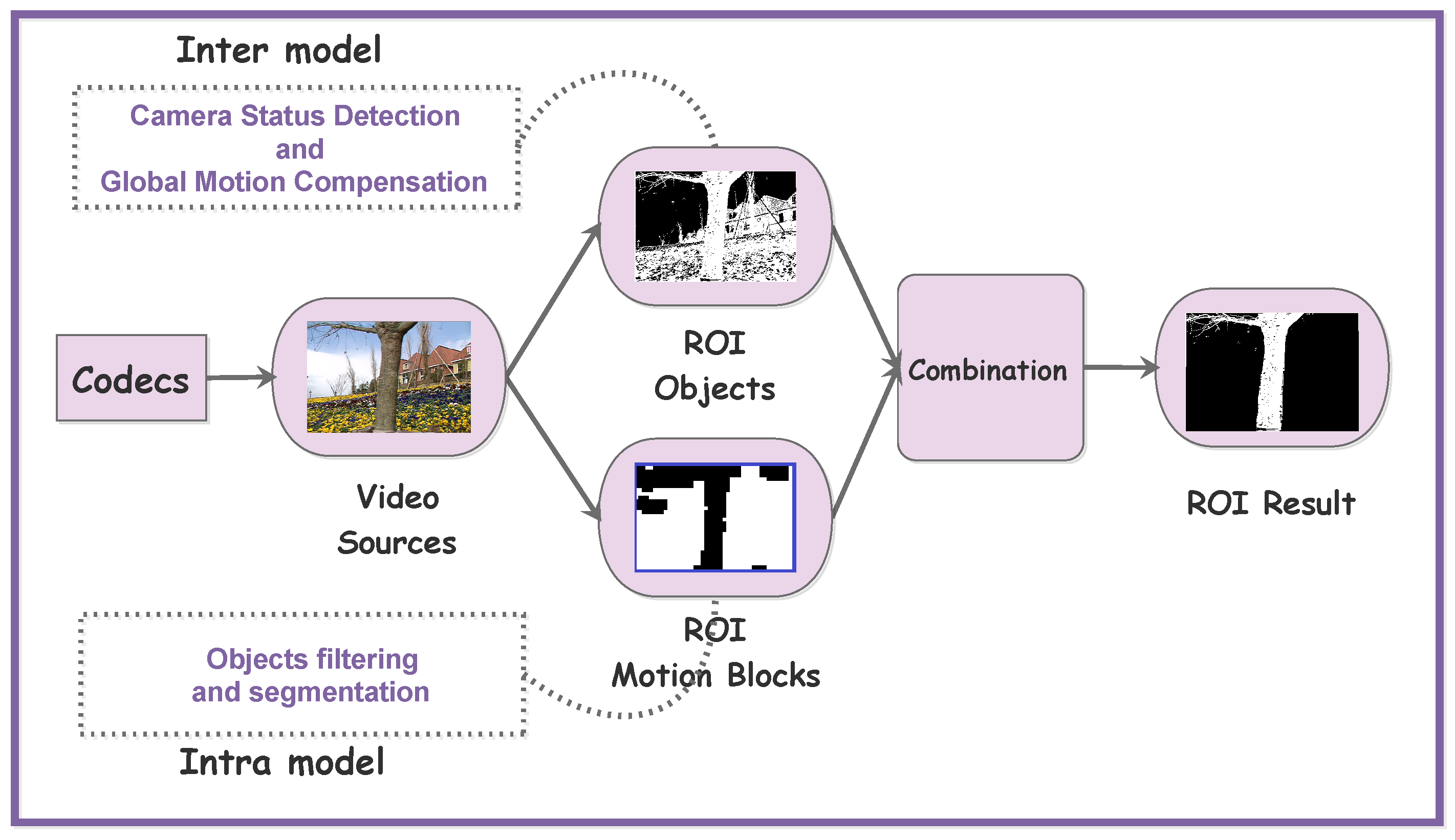
2. Detection Model

2.1. Foreground Motion Blocks Extraction

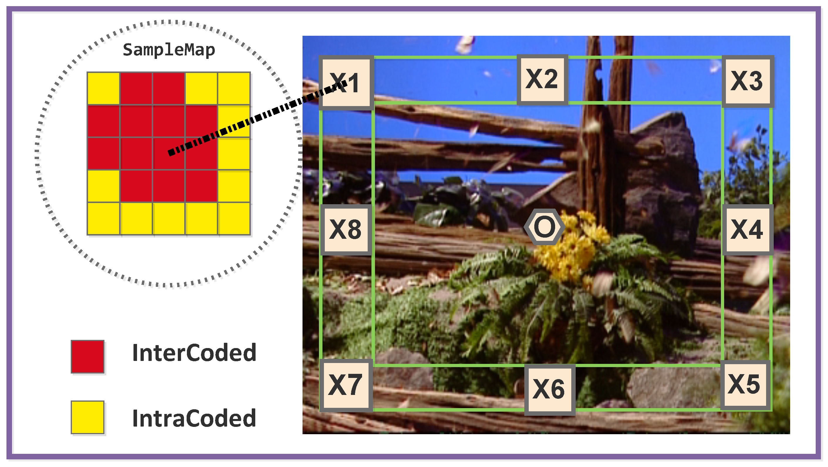
2.1.1. Sampling Areas Determination

We propose a sample-area criteria for a single frame illustrated in Figure 2. There are eight sample areas in a frame, namely, ${\mathit{X}}_1,{\mathit{X}}_2,\cdots {\mathit{X}}_8$, which are located at four diagonal positions and four middle positions in the boundary. Each sample area contains twenty-five $8\times 8$ blocks whose types include both inter and intra, and the size of each sample area is $40\times 40$. The two green rectangles in Figure 2 are represented as the outer and the inner boundary respectively, and the center point in this frame is named as the anchor point. For mathematical analysis, we define sampling set $\mathbb{X}=\{{\mathit{X}}_1,{\mathit{X}}_2,\cdots {\mathit{X}}_8\}$, and each block in ${\mathit{X}}_i(1\le i\le 8)$ is represented as $x_{i1}^i(1\le i1\le 25)$. Also, we define ${\mathbb{I}}_i$ as the intercoded block set and set ${\mathbb{I}}_i^C$ be the intracoded block set for sampling area ${\mathit{X}}_i$. Consider the motion vectors (MVs) for the filtered sampling blocks of the previous frames has a distribution named $q(x)$, and the current unfiltered sampling blocks has a distribution named $p(x)$, we can compute Kullback-Leivler Divergence (KLD) between them as:

$$D(p\parallel q)=E_{x\sim P}\left[log\frac{P(x)}{Q(x)}\right]=\int p(x)log\frac{p(x)}{q(x)}dx,$$

(1)

in which $E_{x\sim P}[·]$ is a statistical average value. To minimize $D(p\parallel q)$, a trick is to quantize these MVs into $\mathbb{X}$ into l levels. Let $m{v}_j^i(j\in {\mathbb{I}}_i)$ denote the jth block’s MV in ${\mathbb{I}}_i$, the maximum and minimum MVs are represented as:

$$\left\{\begin{array}{c}m{v}_{min}(x)=\underset{\bigcup {\mathbb{I}}_i}{min}(\underset{j\in {\mathbb{I}}_i}{min}(m{v}_j^i(x)));m{v}_{min}(y)=\underset{\bigcup {\mathbb{I}}_i}{min}(\underset{j\in {\mathbb{I}}_i}{min}(m{v}_j^i(y)))\hfill \\ m{v}_{max}(x)=\underset{\bigcup {\mathbb{I}}_i}{max}(\underset{j\in {\mathbb{I}}_i}{max}(m{v}_j^i(x)));m{v}_{max}(y)=\underset{\bigcup {\mathbb{I}}_i}{max}(\underset{j\in {\mathbb{I}}_i}{max}(m{v}_j^i(y)))\hfill \end{array}\right.$$

(2)

$mv(x)$ and $mv(y)$ stand for the horizontal and vertical components. The MV step ${\Delta }_s$ equals to $\parallel m{v}_{max}-m{v}_{min}\parallel /l$, where $\parallel ·\parallel$ is the $L_2$ norm. Let $r_s$ be the sth level of the quantized MVs, its probability has the following expression:

$$P_r(r_s)=\frac{n_s}{n},1\le s\le l.$$

(3)

Here, $n_s$ means the number of MVs at level s and n stands for the total quantized MVs. Then, (1) can be rewritten in a discrete way:

$$D(P_r\parallel P_r^{\prime })=\sum _s{P}_r(r_s)log\frac{P_r(r_s)}{P_r^{\prime }(r_s)},$$

(4)

in which $P_r^{\prime }$ is the historical MV distribution for previous frames. Now, we elaborate the proposed sampling block filter algorithm (Algorithm 1):

Algorithm 1 Sampling block filter algorithm

1: Initialize sample set $\mathbb{X}=\varnothing$, $\kappa =1$, l, the expected sample size $S_z$, and the decay factor $\gamma =0.9$. 2: while$|\mathbb{X}|<S_z$do 3:  Reset $\mathbb{X}=\varnothing$. 4:  for $s=1,\cdots ,l$ do 5:   Compute the relative deviation $d=|\frac{\parallel P_r(r_s)-P_r^{\prime }(r_s)\parallel }{P_r(r_s)}|$. 6:   for each intercoded block $x_j^i$ whose MV belongs to level k do 7:    Add $x_j^i$ into $\mathbb{X}$ with an acceptance probability $P_a=1-\kappa d$. 8:   end for 9:  end for 10:  Decrease $\kappa$ by $\kappa =\gamma \kappa$. 11: end while 12: Update $P_r^{\prime }(r_s)$ by rules in (5).

Please note that the algorithm first calculates the relative deviation d between $P_r(r_s)$ and $P_r^{\prime }(r_s)$ at each level and accept each block with a probability according to $\delta$. Next, it maintains the lower bound of the sampling size by reducing $\kappa$ during each loop. Finally, it updates $P_r^{\prime }(r_s)$ by the following rule:

$$P_r^{\prime }(r_s)=\frac{{\displaystyle \sum _i\sum _{j\in {\mathbb{I}}_i}}\delta (x_j^i\notin {\mathbb{I}}_i^{\prime })\delta (Q(m{v}_j^i)=r_s)+n_s^{\prime }}{{\displaystyle \sum _i\sum _{j\in {\mathbb{I}}_i}}\delta (x_j^i\notin {\mathbb{I}}_i^{\prime })+n_s^{\prime }}.$$

(5)

where $\delta (x)$ is the indicator function: $\delta (x)=x\equiv \mathsf{True}?1:0$, ${\mathbb{I}}_i^{\prime }$ is the previous sampled intercoded block set of the ith area, $n_s^{\prime }$ stands for the previous number of sampled blocks, and $Q(mv)$ represents the quantized level of a MV. Please note that the updating rule recalculates $P_r^{\prime }(r_s)$ by updating the previous and current sampling sets with different sampling blocks. At the first P-frame, all the intercoded blocks in ${\mathit{X}}_i$ are added into sampling set $\mathbb{X}$. Then, the filter algorithm reduces the “error” blocks via an updating process to get the correct sampling blocks for global motion detection.

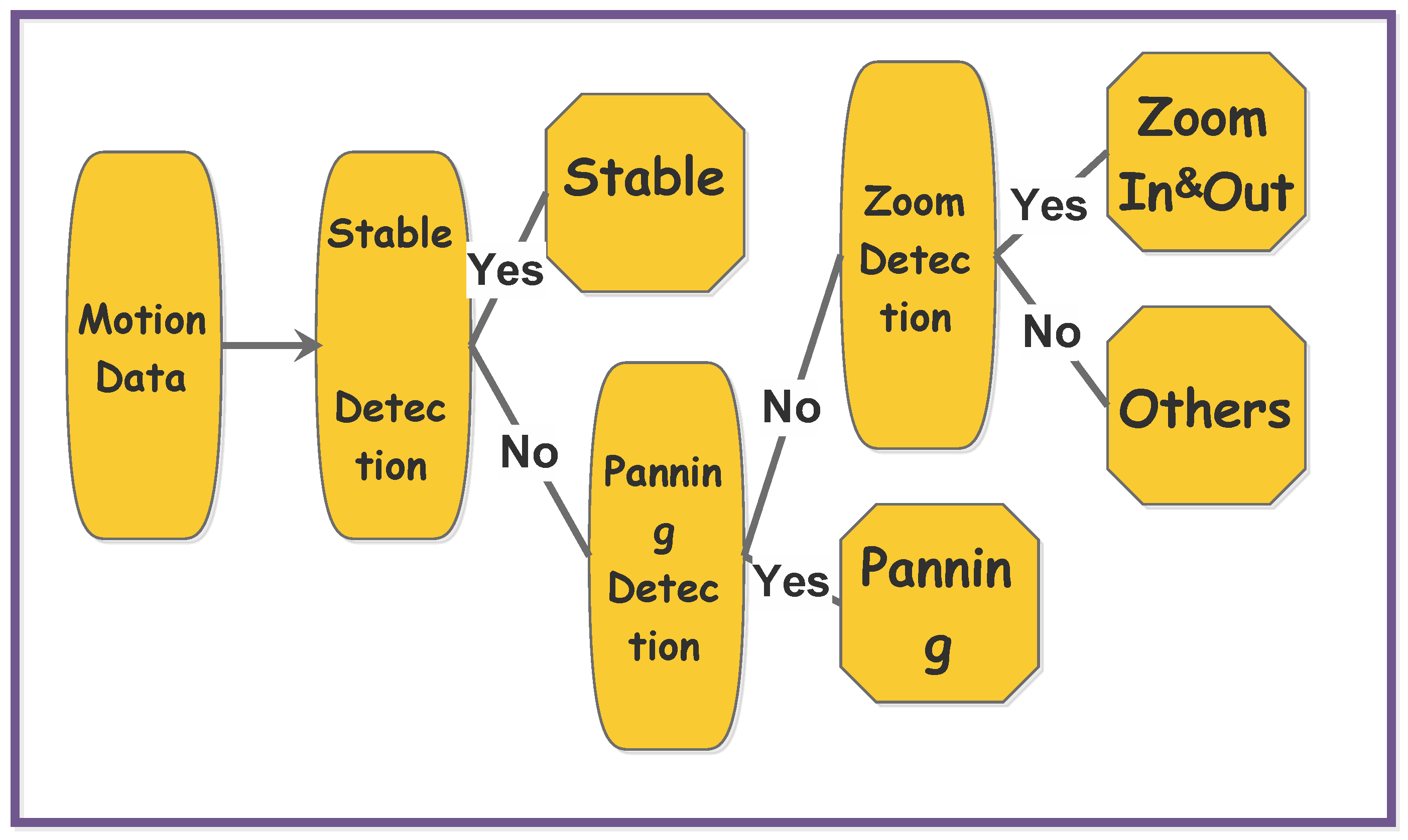
2.1.2. Camera Status Detection

The global motion estimation (GME) method handles for these situations specifically: stable, camera panning, camera zoom in/out and others. A status assemble $\mathcal{H}=\{C_s,C_p,C_{zi},C_{zo},C^{\prime }\}$ is defined according to the listed situations. Each camera state and its decision model are demonstrated in details:

• Panning
  To determine Camera Panning, an intuitive approach is to compare the norm and direction of MVs among different sampling areas. For each area ${\mathit{X}}_i$, its average MV value is computed as follows:

  $$\left\{\begin{array}{cc}\overline{m{v}_i}(x)\hfill & =\frac{1}{|{\mathbb{I}}_i|}{\displaystyle \sum _{j\in {\mathbb{I}}_i}}m{v}_j(x)\hfill \\ \overline{m{v}_i}(y)\hfill & =\frac{1}{|{\mathbb{I}}_i|}{\displaystyle \sum _{j\in {\mathbb{I}}_i}}m{v}_j(y)\hfill \end{array}\right.$$

  (6)

  We define MV set $\mathcal{MV}(\mathbb{X})=\{\overline{m{v}_1},\cdots ,\overline{m{v}_8}\}$. For normalization, we have:

  $$\left\{\begin{array}{cc}\overline{m{v}_i}(x)\hfill & =\overline{m{v}_i}(x)/(m{v}_{max}(x)-m{v}_{min}(x))\hfill \\ \overline{m{v}_i}(y)\hfill & =\overline{m{v}_i}(y)/(m{v}_{max}(y)-m{v}_{min}(y))\hfill \end{array}\right.$$

  (7)

  and their variance without the minimum and maximum values are listed below:

  $$\begin{array}{c}\hfill \left\{\begin{array}{c}Var(mv(x))=\frac{1}{N}{\displaystyle \sum _{i\in \mathcal{MV}(\mathbb{X})}}{(\overline{m{v}_i}(x)-\overline{mv}(x))}^2\hfill \\ Var(mv(y))=\frac{1}{N}{\displaystyle \sum _{i\in \mathcal{MV}(\mathbb{X})}}{(\overline{m{v}_i}(y)-\overline{mv}(x))}^2\hfill \end{array}\right.\end{array}$$

  (8)

  Please note that $\overline{mv}(·)$ denotes the average values of $\overline{m{v}_i}(·)$, and N equals to the size of $\mathcal{MV}(\mathbb{X})$. Meanwhile, the angle components of $\mathcal{MV}(\mathbb{X})$ are taken into consideration as well. Let ${\theta }_i$ be the angle component for $\overline{m{v}_i}(x)$:

  $${\theta }_i=arctan\frac{|\overline{m{v}_i}(x)|}{|\overline{m{v}_i}(y)|},$$

  (9)

  and its variance is followed by:

  $$Var(\theta )=\frac{1}{N}\sum _i{({\theta }_i-\overline{\theta })}^2(1\le i\le N).$$

  (10)

  Then, a score parameter $S_{cp}$ for judging camera panning is formed as:

  $$S_{cp}=[1-\frac{1}{2}(Var(mv(x))+Var(mv(y)))]{|ln(1-Var(\theta ))+1|}^{-1}.$$

  (11)

  $S_{cp}$ is within a range of (0,1) since normalization process is done before calculation, and $ln(1-Var(\theta ))$ is treated as the penalty function. When $Var(\theta )\to 1$, $S_{cp}\simeq 0$ since we attempt to put more weight on the variance of $\theta$ to decide the camera panning circumstance.
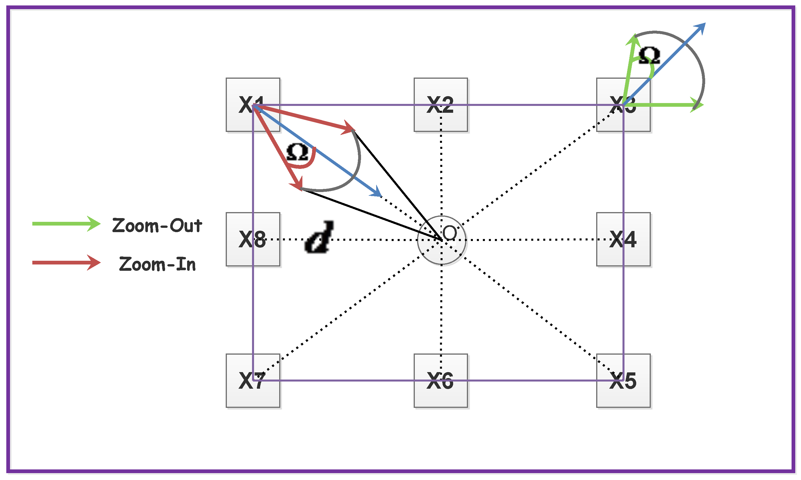
• Zoom-In and Out:
  In this status, each sampling area has a different direction of motion vector. An illustration for the zooming model is displayed in Figure 3.
  Obviously, the directions of motion vectors for these sampling areas can be regarded as a factor to determine the zooming in and out situation. Also, the norm of motion vectors is relevant with the distance between the anchor point and each center of the character block. To be specific, we categorize $\mathbb{X}$ into two groups: ${\mathbb{X}}_{diag}=\{{\mathit{X}}_1,{\mathit{X}}_3,{\mathit{X}}_5,{\mathit{X}}_7\}$ and ${\mathbb{X}}_{mid}=\{{\mathit{X}}_2,{\mathit{X}}_4,{\mathit{X}}_6,{\mathit{X}}_8\}$. Also, define a set of vectors $\mathbb{F}=\{{\overrightarrow{f}}_1,{\overrightarrow{f}}_2,\dots ,{\overrightarrow{f}}_N\}$ that:

  $${\overrightarrow{f}}_i=(X_o-{\mathit{X}}_i(x),Y_o-{\mathit{X}}_i(y)){\mathit{X}}_i\in \mathbb{X},$$

  (12)

  where $(X_o,Y_o)$ is the coordinate of the anchor point o, and $({\mathit{X}}_i(x),{\mathit{X}}_i(y))$ is the mean coordinate of ${\mathit{X}}_i$. For camera zoom-in status, the inner product of $\mathcal{MV}(\mathbb{X})$ and $\overrightarrow{f}$ is a positive value while it is negative in zoom-out status. We can compute the offset angle $\Omega$ for zoom in and out by:

  $${\Omega }_i=arccos\frac{\overline{m{v}_i}·{\overrightarrow{f}}_i}{\mid \overline{m{v}_i}\mid \mid {\overrightarrow{f}}_i\mid }.$$

  (13)

  Apparently, ${\Omega }_i>0$ means ${\mathit{X}}_i$ is in the direction of zoom-in, otherwise zoom-out. We keep $\Omega$ in a belief range $[{\Omega }_l,{\Omega }_r]$, in which the max difference between ${\Omega }_r$ and ${\Omega }_l$ is set assigned with a constant value (marked in Figure 3 as gray solid arcs). Suppose $\Omega$ obeys the normal distribution: $\Omega \sim \mathcal{N}(\mu ,\sigma )$. Then, the likelihood factor $\mathcal{L}$ is given as:

  $$\left\{\begin{array}{cc}\mathcal{L}(\Omega )\hfill & =2\pi {\sigma }^{-\frac{1}{2}}exp(\frac{{(\Omega -\mu )}^2}{2{\sigma }^2})\hfill \\ \tilde{\mathcal{L}}(\Omega )\hfill & =\mathcal{L}(\Omega )/\mathcal{L}(\mu ).\hfill \end{array}\right.$$

  Please note that $\tilde{\mathcal{L}}(\Omega )$ is normalized to unify the range. Besides, a ’hit and miss’ voting scheme is induced: for the zoom-in situation, if ${\Omega }_i>\sigma$, we say that sampling area i misses the zoom-in contribution, otherwise hit; for the zoom-out situation, if $\pi -{\Omega }_i>\sigma$, we say miss, otherwise hit. Now, the voting rate for zooming situation is declared as:

  $$V(\mathbb{X})=\frac{1}{N}\sum _i\delta ({\Omega }_i,\sigma )1\le i\le N$$

  (14)

  where $\delta ({\Omega }_i,\sigma )$ is also an indicator function:

  $$\delta ({\theta }_i,\sigma )=\left\{\begin{array}{cc}1\hfill & {\Omega }_i<\sigma and\overline{m{v}_i}·{\overrightarrow{f}}_i>0\hfill \\ -1\hfill & \pi -{\Omega }_i<\sigma and\overline{m{v}_i}(x)·{\overrightarrow{f}}_i<0\hfill \\ 0\hfill & otherwise.\hfill \end{array}\right.$$

  (15)

  When $|V({\mathit{X}}_i)|\ge p$, the voting rate’s error is given as $1-p$. It can be seen that the sampling areas with opposite motion directions show more negative contributions on $V(\mathit{X})$ than ones with higher variances, which is reasonable since motion direction plays an important role in zoom judging. Another factor that influences zoom judging is the norm of $\mathcal{MV}(\mathbb{X})$, it satisfies:

  $$E(|\overline{\mathcal{MV}({\mathbb{X}}_{diag})}|)\simeq \frac{h}{\sqrt{w^2+h^2}}E(|\overline{\mathcal{MV}({\mathbb{X}}_{mid})}|),$$

  (16)

  where w and h are width and height of a frame, $|\overline{\mathcal{MV}({\mathbb{X}}_{diag})}|$ stands for the average norm of MVs in ${\mathbb{X}}_{diag}$. Observe that this equation is the approximate one, and its relative error $\epsilon$ can be defined as:

  $$\epsilon =\frac{2|E(|\overline{\mathcal{MV}({\mathbb{X}}_{diag})}|)-\frac{h}{\sqrt{w^2+h^2}}E(|\overline{\mathcal{MV}({\mathbb{X}}_{mid})}|)|}{E(|\overline{\mathcal{MV}({\mathbb{X}}_{diag})}|)+\frac{h}{\sqrt{w^2+h^2}}E(|\overline{\mathcal{MV}({\mathbb{X}}_{mid})}|)}$$

  (17)

  Finally, the score for deciding camera zooming is given below:

  $$S_z=\frac{(1-\epsilon )V(\mathbb{X})}{N}\sum _i\tilde{\mathcal{L}}(\Omega )(1\le i\le N)$$

  (18)

  When $S_z$ is negative, it is inclined to zoom-out situation, otherwise zoom-in. In addition, we have to set a threshold $t_h$ that must satisfy $|S_z|>t_h$ for the zooming circumstances.
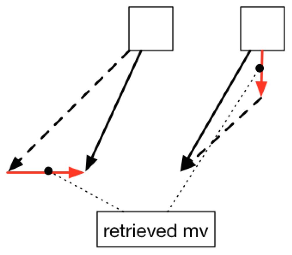
• Stable and Others:
  For a stable situation, it is easy to judge by checking whether $E(|V(\mathbb{X})|)\simeq 0$ or $Var(|\mathcal{MV}(\mathbb{X}|)\simeq 0$. Besides, the sampling set $\mathbb{X}$ contains most of intracoded blocks ($|{\mathbb{I}}^C|\gg |\mathbb{I}|$), which indicates the stable situation as well. The last circumstances $C^{\prime }$ is named as “rest” when it does not satisfy any of the above circumstances. Please note that $C^{\prime }$ may consist some important situations that we have ignored in previous detection steps. For example, the combination of panning and zooming, which occurs frequently in video recording. It is hard to decompose both panning and zooming motion vector component since the panning component can have any directions and norms. An alternative way is to simplify this problem by extracting the horizontal and vertical panning motion vectors from the composed one separately. We consider the upper-right corner sampling area in Figure 4 for instance, solid lines represent the extracted motion vectors, and they can be forced to decompose into the zoom-in and the retrieved horizontal/vertical components (dotted lines and red solid lines). The norm of the zoom-in component is set as a fixed value to make sure the retrieved motion vector is horizontal or vertical. We re-compare the retrieved horizontal and vertical components for the sampling areas using the camera panning model; if it satisfies the conditions, the status of camera is both panning and zooming. On the other hand, the zoom-out situation follows the same rule as the zoom-in.

We propose a decision tree model is designed for global motion detection, as depicted in Figure 5.

Also, a related algorithm is written in Algorithm 2.

Algorithm 2 Global motion decision algorithm

1: if ($E(|V(\mathbb{X})|)\simeq 0$ and $Var(|V(\mathbb{X})|)\simeq 0$) or $|{\mathbb{I}}^C|\gg |\mathbb{I}|$, return $C_s$. 2: Compute $S_{cp}$ using (11), if $S_{cp}>t_{h1}$, return $C_p$. 3: Compute $S_z$ using (18), if $|S_z|>t_{h2}$ and $S_z>0$ return $C_{zi}$. 4: else if$|S_z|>t_{h2}$ and $S_z<0$ return $C_{zo}$. 5: else return$C^{\prime }$.

The tree is mainly classified into three categories: stable, panning, zooming, and they are ordered by occurrence probabilities. Threshold $t_{h1}$ and $t_{h2}$ are induced to control the detection precision.

2.1.3. Global Motion Compensation

A global motion compensation procedure is recommended for each block to retrieve the foreground MVs. Since the coding unit (CU) has different resolutions both in VPX and in HEVC, it is recommended to unify the block size for processing as $8\times 8$. For each block $b_i$ in a frame, its compensated motion vector is computed through:

$$m{v}_r(b_i)=mv(b_i)-m{v}_g(b_i),$$

(19)

where $m{v}_r(b_i)$ and $m{v}_g(b_i)$ denote the real and global motion vector respectively. The key problem is to compute $m{v}_g$ for each block $b_i$ in different camera circumstances. Consider each element $h\in \mathcal{H}$, for $h=C_s$, $m{v}_r(b_i)=mv(b_i)$; For $h=C_p$, $m{v}_g(b_i)=E(\mathcal{MV}(\mathbb{X}))$; For $h=C_{zo}$ and $h=C_{zi}$, according to Figure 3, it might be asserted that $m{v}_g(b_i)$ and $\overrightarrow{f_{bi}}$ have the same or opposite directions, in other words, $\frac{m{v}_g(b_i)·\overrightarrow{f_{bi}}}{|m{v}_g(b_i)||\overrightarrow{f_{bi}}|}\simeq \pm 1$. When $h=C_{zi}$, $m{v}_g(b_i)=\alpha \overrightarrow{f_{bi}}$, and when $h=C_{zo}$, $m{v}_g(b_i)=-\alpha \overrightarrow{f_{bi}}$. $\alpha$ denotes the scaling factor, which has the following expression:

$$\alpha =\frac{1}{N}\sum _{i=0}^N\frac{|\overline{m{v}_i}|}{|{\overrightarrow{f}}_i|}.$$

(20)

Last but not least, if $h=C^{\prime }$, we check whether the combination of panning and zooming occurs first, if so, $m{v}_g(b_i)$ is composed of the two motion vectors and $m{v}_r(b_i)$ can be acquired by (19) and (20). Otherwise, it is recommended to check out the previous result of h in the reference frame buffer for the current one. If the current one is I frame (has no reference frame), or $h_{ref}=C^{\prime }$ without combining the cases of panning and zooming, we have to ignore $m{v}_g(b_i)$ and leave it as zero since lacking of global motion information. If $h_{ref}\ne C^{\prime }$, we use $m{v}_g{(b_i)}^{\prime }$ of the reference frame instead of this one as the last choice.

2.1.4. Discussion

Figure 6 displays some extracted motion blocks for ROI foreground objects via different approaches. Each method is introduced in brief:

• Gradient-Descent (GD) [63]: It aims to compute the gradient by Newton-Raphson method for the error distance between the true and the estimated MVs, then it updates parameters based on the gradient descend direction so that the error distance is reduced.
• Least-Sum-Square M-Estimator (LSS-ME) [64]: It involves formulating the error distance by an over-determined regression: ${\mathit{A}}^T\mathit{A}\mathit{m}={\mathit{A}}^T\mathit{b}$, where $\mathit{A}\in {\mathbb{R}}^{2N\times 8}$, $\mathit{b}$ is a $2N$ vector of transformed coordinates $(x^{\prime },y^{\prime })$, and N is the total number of MVs. It also uses iterative outlier rejection through a robust M-Estimator to estimate motion components $\mathit{m}$.
• RANSAC [65]: This method induces a statistical method for GME in different computer vision problems. It computes the homography matrix via a large number of iterations to achieve the maximum transformed matching points between the current and the reference frames.

One can see that the proposed method retrieves the foreground MV blocks more accurately than others by eliminating “noisy” background blocks. Instead of using the regression (GD, LSS-ME) or statistical (RANSAC) methods to estimate the global motion parameter $\mathit{m}$, the proposed decision tree model is efficient on judging the global camera status. The average running time (sec/frame) performances are tested on OpenCV (C++) with a 2.8GHZ Core i7 CPU.

Table 1. Running time tests for GME approaches. (Platform: OpenCV 3.1, Core-i7 CPU 2.8GHZ × 4).

Sequences	Our Method	GD	LSS-ME	RANSAC
Flower	0.097 s	0.181 s	0.466 s	0.240 s
Stefan	0.293 s	0.665 s	0.712 s	0.497 s
CoastGuard	0.225 s	0.604 s	0.811 s	0.472 s

displays that the proposed method achieves a better result in time performance since high computation costs of matrix SVD and iterations are substituted by the tree model with $O(n)$ complexity.

To justify how these thresholds influence the classifier’s performance, several sequences are collected for test with different characteristics. These sequences are pre-analyzed by the photographer’s comments for status judgements, and any decision result which obeys the objective comments is treated as the misjudgement. For performance evaluation purpose, we extract partial frames in each sequence to ensure that each sequence has at least two camera states. Frames with main status are regarded as positive samples while others are negative samples. Without loss of generality, we select the number of negative samples nearly the same as the positive ones. For example, in foreman, frames between 47–81 are commented as the stable state and 82–115 are commented as the panning state.

Table 2. Performance of camera status decision with different settings of thresholds.

Seq	Status	$\mathit{th}1$	$\mathit{th}2$	prec	Recall	F-Score
BQTerrace Flower Foreman	panning /rests	0.1	0.3	0.818	0.901	0.857
		0.3	0.3	0.940	0.901	0.922
		0.5	0.3	0.846	0.880	0.863
		0.7	0.3	0.702	0.801	0.747
PartyScene BQSquare Mobile	zooming /rests	0.3	0.1	0.649	0.740	0.692
		0.3	0.3	0.722	0.780	0.750
		0.3	0.5	0.773	0.820	0.796
		0.3	0.7	0.693	0.680	0.686

displays some performance indexes (e.g., recall, precision, F-score) for different settings of threshold $th1$ and $th2$. The panning and zooming groups are tested with six sequences, and the results are acquired by computing their average values. One can see that an optimal combination of ($th1$, $th2$) is (0.3, 0.5), which indicates that the classifier is able to make acceptable decisions for camera statuses.

2.1.5. Marking Motion Areas

After acquiring the global compensated motion data of foreground ROI objects, a MV clustering method is proposed to segment blocks into motion areas. For each ROI block, we apply the target clustering function J based on the following definition:

$$J=\sum _{i=1}^N\sum _{j=1}^K{\mu }_{ij}(\parallel {\tilde{x}}_i^p-{\tilde{c}}_j^p{\parallel }^2+\parallel {\tilde{x}}_i^{mv}-{\tilde{c}}_j^{mv}{\parallel }^2+\parallel {\tilde{x}}_i^I-{\tilde{c}}_j^I{\parallel }^2),$$

(21)

where ${\tilde{x}}_i^p$, ${\tilde{x}}_i^{mv}$ and ${\tilde{x}}_i^I$ denote the normalized vectors of position, motion vector, pixel intensity for block i correspondingly. Please note that ${\tilde{x}}_i^I$ has three components (Y/U/V) while the others have two. ${\mu }_{ij}$ indicates the belongingness of block i to cluster area j, and c stands for the center vector. Apparently, the target function J considers blocks’ position together with pixel and motion similarities. To solve non-spherical clusters, we use Kernel Fuzzy C-Means (KFCM) method for block classification, which induces the kernel function $\mathcal{K}({\tilde{\mathit{x}}}_i,{\tilde{\mathit{c}}}_j)=exp(-\frac{\parallel {\tilde{\mathit{x}}}_i-{\tilde{\mathit{c}}}_j{\parallel }^2}{{\sigma }^2})$ in criteria computation. To adaptively classify these foreground blocks, we propose a clustering algorithm which optimally classifies blocks into adequate areas, see Algorithm 3 for details.

Algorithm 3 KFCM Motion Areas Clustering Algorithm

1: Set $k=1$, ${\tilde{\mathit{c}}}_1=E({\tilde{\mathit{x}}}_i^p,{\tilde{\mathit{x}}}_i^{mv},{\tilde{\mathit{x}}}_i^I)$. 2: while$k\ge K_{max}$do 3:  Segment N blocks into k clusters by KFCM algorithm with the stopping criteria: $\frac{|J^{t+1}-J^t|}{J^t}<ϵ$. 4:  Compute $J_j={\displaystyle \sum _{i=1}^{|{\tilde{\mathit{c}}}_j|}}(\parallel {\tilde{x}}_i^p-{\tilde{c}}_j^p{\parallel }^2+\parallel {\tilde{x}}_i^{mv}-{\tilde{c}}_j^{mv}{\parallel }^2+\parallel {\tilde{x}}_i^I-{\tilde{c}}_j^I{\parallel }^2)$. 5:  if ${max}_{j\in (0,k]}{J}_j<\epsilon |{\tilde{\mathit{c}}}_j|$ and $|{\tilde{\mathit{c}}}_j|\ge N/(k+o)$ then 6:   return $\mathit{\mu }$, k, ${\tilde{\mathit{c}}}_j,j\in (0,k]$. 7:  end if 8:  $k=k+1$; 9: end while 10: return$\mathit{\mu }$, $K_{max}$, ${\tilde{\mathit{c}}}_j,j\in (0,K_{max}]$.

Notice that the clustering algorithm segments the foreground blocks into k clusters, where k increases from 1 to $K_{max}$ iteratively. At each turn, it computes the target function ($J_j$) for each cluster j. When each cluster’s size satisfies that $|{\tilde{\mathit{c}}}_j|\ge N/(k+o)$ (o is an offset, empirically set as 2) and $J_j$ is constrained on a upper bound $\epsilon |{\tilde{\mathit{c}}}_j|$, the algorithm stops and returns the optimal cluster labels.

To specify the parameter influences on segmentation results, we set $K_{max}=4$ and change $\epsilon$ from 0 to 1. The clustering results are displayed in Figure 7, whereas three sequences are included for comparisons. We find that when $\epsilon \ge 0.25$, the algorithm outputs two clusters; as $\epsilon$ decreases, more clusters are generated with margin details. Next, we collect the margin points for each cluster. Let us assume that ${\mathfrak{M}}_i=\{b_t,b_l,b_r,b_b\}$, in which collection ${\mathfrak{M}}_i$ contains the top, left, right and bottom block for cluster i. Then, a rectangle area can be drawn based on these blocks. However, some “noise” blocks may reduce the precision of determining ${\mathfrak{M}}_i$. For example, in Figure 8c, the rectangle area covers many blank areas that are useless. To solve this problem, we propose a motion area pruning algorithm, see Algorithm 4 for details. Please note that the algorithm first traverses each block cluster from its margin points in a depth-first way. The searching procedure terminates when it reaches the bounds or the visiting block is not ROI block ($R^n$). Then, the traversed data is collected into subset $\mathcal{B}$. If the size of $\mathcal{B}$ is small enough, the blocks in $\mathcal{B}$ are ignored as “noise” ones. Finally, the algorithm returns the pruned block set ${\mathcal{B}}_1$. Please note that the search range r and step s are set as five and two block-distance empirically, in which larger value of r would eliminate less “noise” blocks. Figure 8 shows the boundaries of motion areas before and after the pruning algorithm. We can observe that the proposed method reduces the “noise” blocks effectively and obtains the precise rectangle.

Algorithm 4 Motion Area Pruning Algorithm

$Search(b,Vis,\mathcal{B})$:

Input:b: The current processing block; $Vis$: Whether the block is visited; $\mathcal{B}$: Temp block lists; Search range r and step s. 1: If$CheckBound(b)==$false or$Vis(b)$or$Type(b)==R^n$, return. 2: $Vis(b)$=true, append b to B. 3: for$i=1$; $i<r$; $i+=s$do 4:  $Search(b(x\pm i,y\pm i),Vis,\mathcal{B})$. 5: end for

$Prune(\mathfrak{M})$:

Input: : Margin block set $\mathfrak{M}$; Original block set ${\mathcal{B}}_0^i$. Pruned block set ${\mathcal{B}}_1^i=\varnothing$ ($0<i\le k$). 1: for each${\mathfrak{M}}_i$in$\mathfrak{M}$do 2:  for each $b_j$ in ${\mathfrak{M}}_i$ do 3:   $Search(b_j,Vis,{\mathcal{B}}_j)$. 4:   If $|{\mathcal{B}}_j|>\frac{{\mathcal{B}}_0^i}{|{\mathfrak{M}}_i|+o}$, ${\mathcal{B}}_1^i\bigcup ={\mathcal{B}}_j$. 5:  end for 6: end for 7: return$\bigcup {\mathcal{B}}_1^i$.

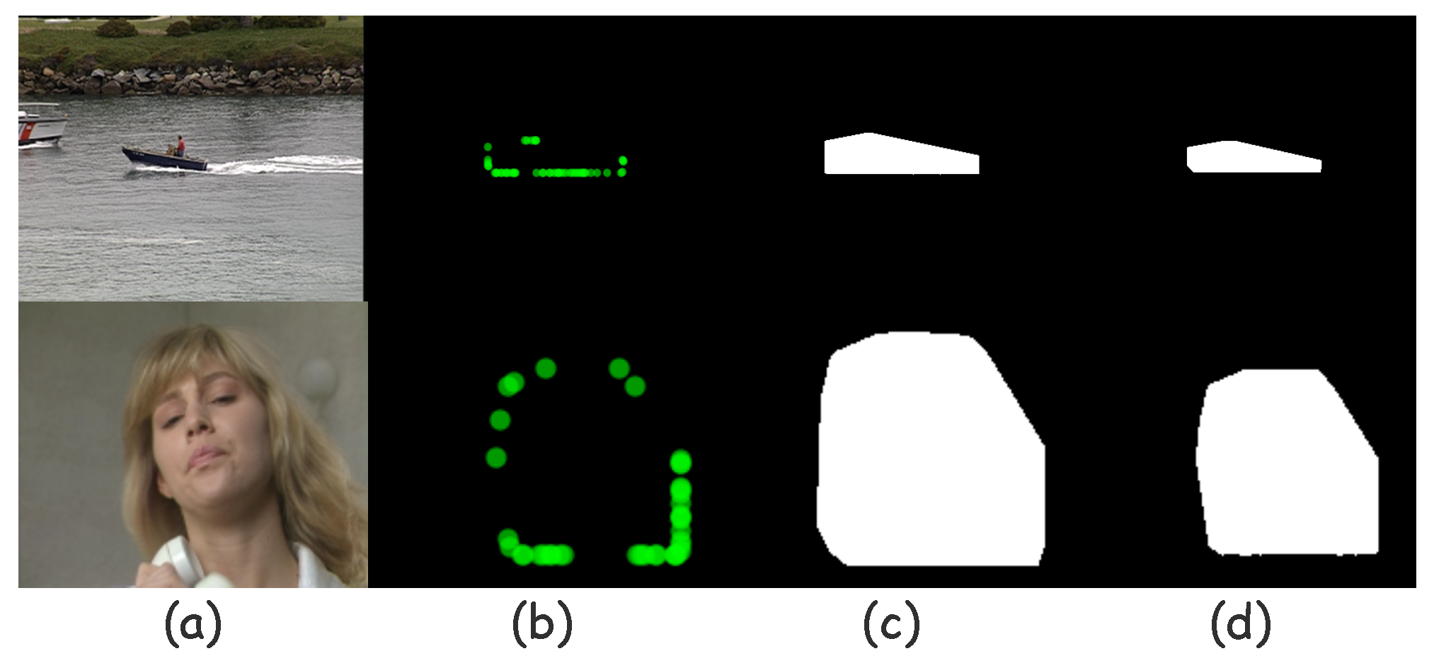
2.1.6. Mask Drawing and ROI Extracting

After obtaining the boundaries of motion areas for each cluster, we consider drawing the margin masks for the motion areas. First of all, the “edge” blocks of each cluster are filtered by edge detection methods (i.e., Canny, Sobel). Let us assume that ${\mathcal{B}}_E^i$ is the set of “edge” blocks of the ith cluster, the shape of mask is then generated by the Gift-Wrapping algorithm in [66], see Figure 9 for details.

Please note that the Gift-Wrapping algorithm performs as a convex hull scan method, in which the convex shape of the motion area is clearly formed. For alternating the cover area, we define the center of motion area i as:

$${\mathcal{C}}_m^i(r,c)=\frac{1}{|{\mathcal{B}}_E^i|}\sum _{b_E\in {\mathcal{B}}_E^i}{b}_E(r,c),$$

(22)

where ${\mathcal{C}}_m^i(r,c)$ denotes the center coordinate ($(r,c)$ means row and column). We also declare an inflation factor $\iota$ which controls the scaling extent of the mask. Given a fixed $\iota$, the updated “edge” blocks $b_E^{\prime }(r,c)$ can be expressed as:

$$\left\{\begin{array}{cc}{b}_E^{\prime }(r)\hfill & =b_E(r)+(\iota -1)·(b_E(r)-{\mathcal{C}}_m(r))\hfill \\ b_E^{\prime }(c)\hfill & =b_E(c)+(\iota -1)·(b_E(c)-{\mathcal{C}}_m(c))\hfill \end{array}\right.$$

(23)

To specify how $\iota$ influences the mask shape, we change $\iota$ from 1 to 1.4, the visual effects of which is displayed in Figure 9c,d. After acquiring the mask data, we can determine the result of foreground objects inside the mask. We use the extracting method in our previous work [14], it implements a multidimensional segmentation method with the Expectation Maximization (EM) algorithm to segment the mask data into an optimal number of clusters. Then, for each cluster inside the mask, it computes the KLD ($D(p_b\parallel p_f)$) between the background pixel histogram $p_b(x)$ and foreground pixel histogram $p_f(x)$. When $D(p_b\parallel p_f)$ is below a threshold ${\xi }_x$, the current cluster is treated as the background cluster and it is removed from the mask. At the end of each iteration, $p_b$ is updated based on the removed clusters and sampling background blocks, see Formula 25 in our previous work [14] for details.

3. Experiments

3.1. Visual Effect Analysis Experiments

3.1.1. Parameters Settings

It is essential to set some parameters before performing the visual analysis experiment. For ROI inter model, two threshold $th1$ and $th2$ are set to 0.5 empirically since the score is normalized, and the norm of the real motion vector should satisfy $\parallel m{v}_{b_i}\parallel >\sqrt{2}$ as a condition to determine whether block $b_i$ belongs to motion mask $\mathcal{M}$. For ROI intra model, the initial value of $\vartheta (\mathit{\tau },\mathit{\mu },\mathbf{\Sigma })$ is set manually instead of a random value for reducing iteration steps. Practically, $\mathit{\tau }$ is set initially as $\{0.5,0.5\}$ for $K=2$ classes, and $\mathit{\mu }$, $\mathbf{\Sigma }$ are recommend to be acquired by running the K-means cluster ($K=2$) method first and use the outputs as their initial values. ${\mathit{z}}_i$ is assigned by an uniform distributed binary array $\{0,1,0,1,\dots \}$ with the same probability for each value. $\beta$ is set as 1.5 and ${\xi }_1,{\xi }_2$ are initiated as 8 and 0.12 respectively. Besides, the max-iteration steps for EM algorithm are constrained to 10 for reducing the computing costs.

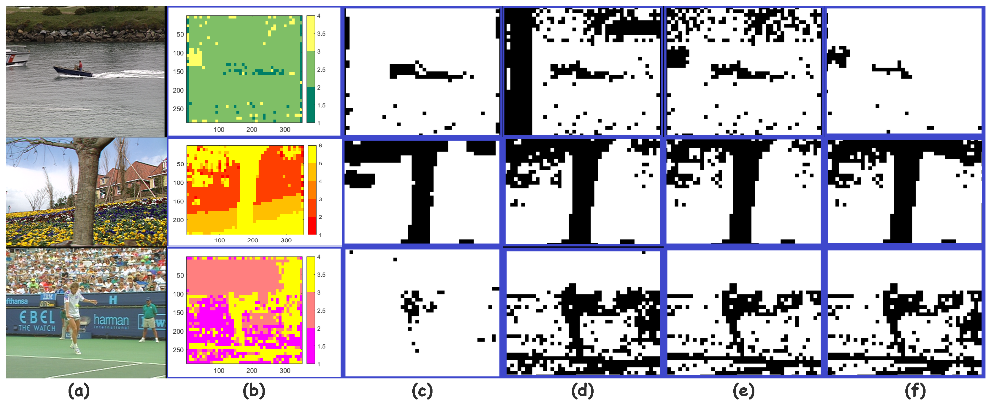
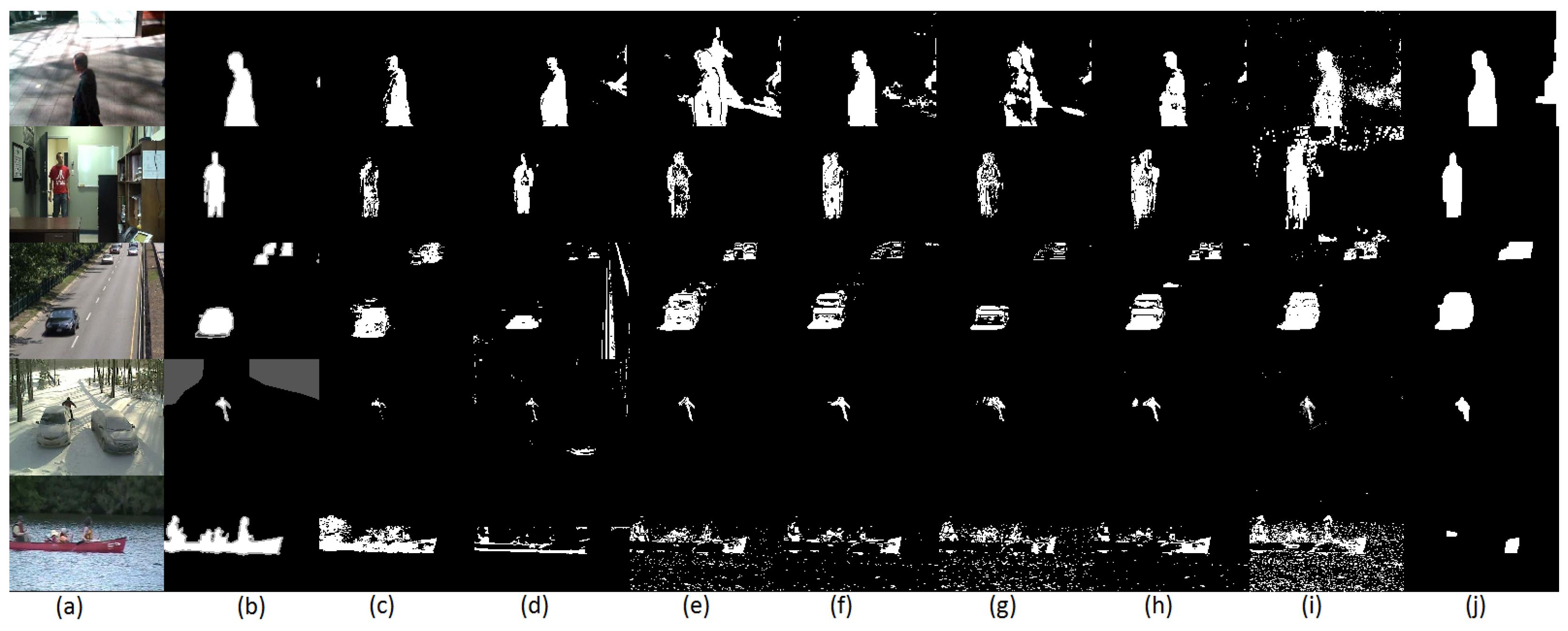
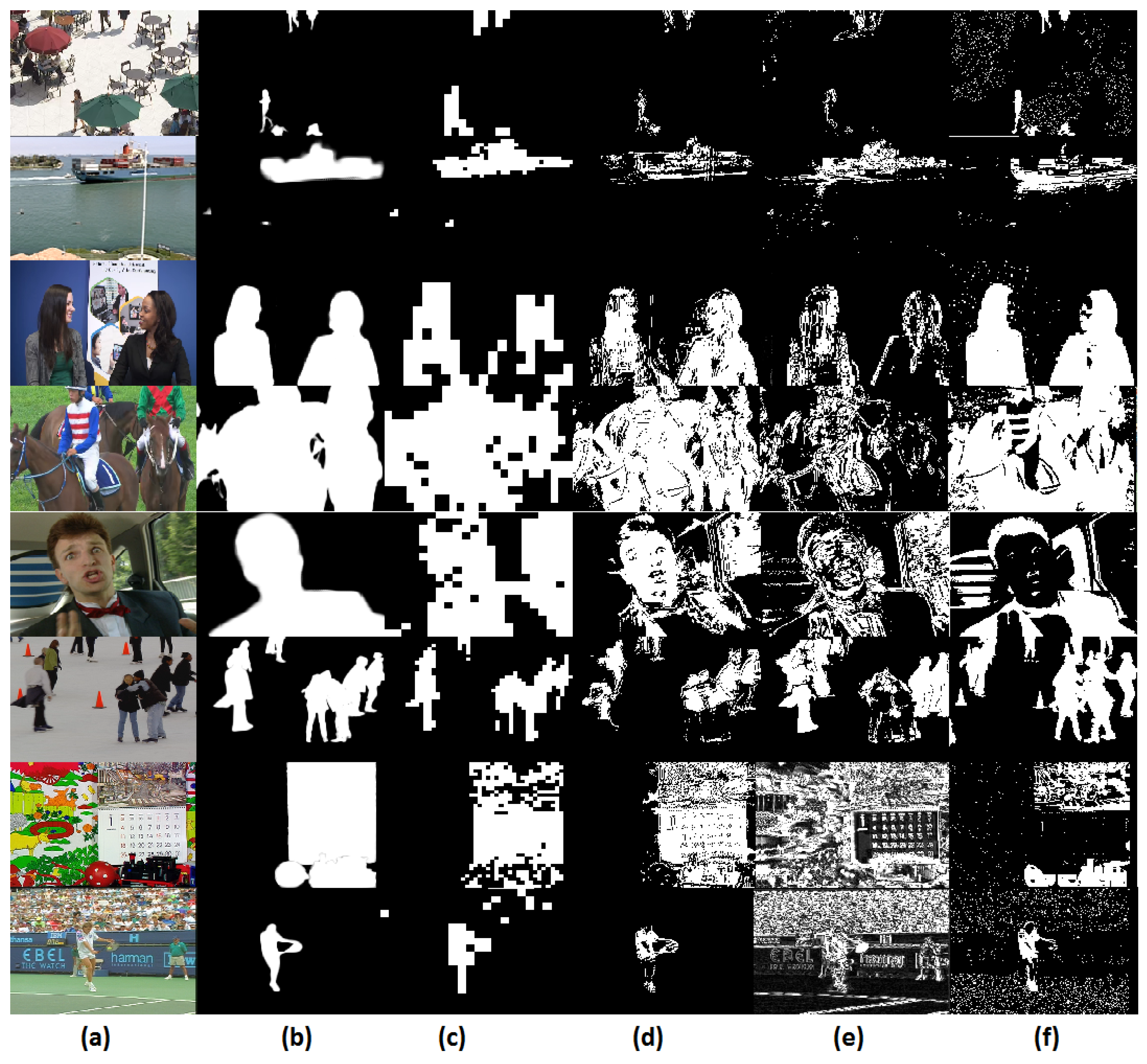
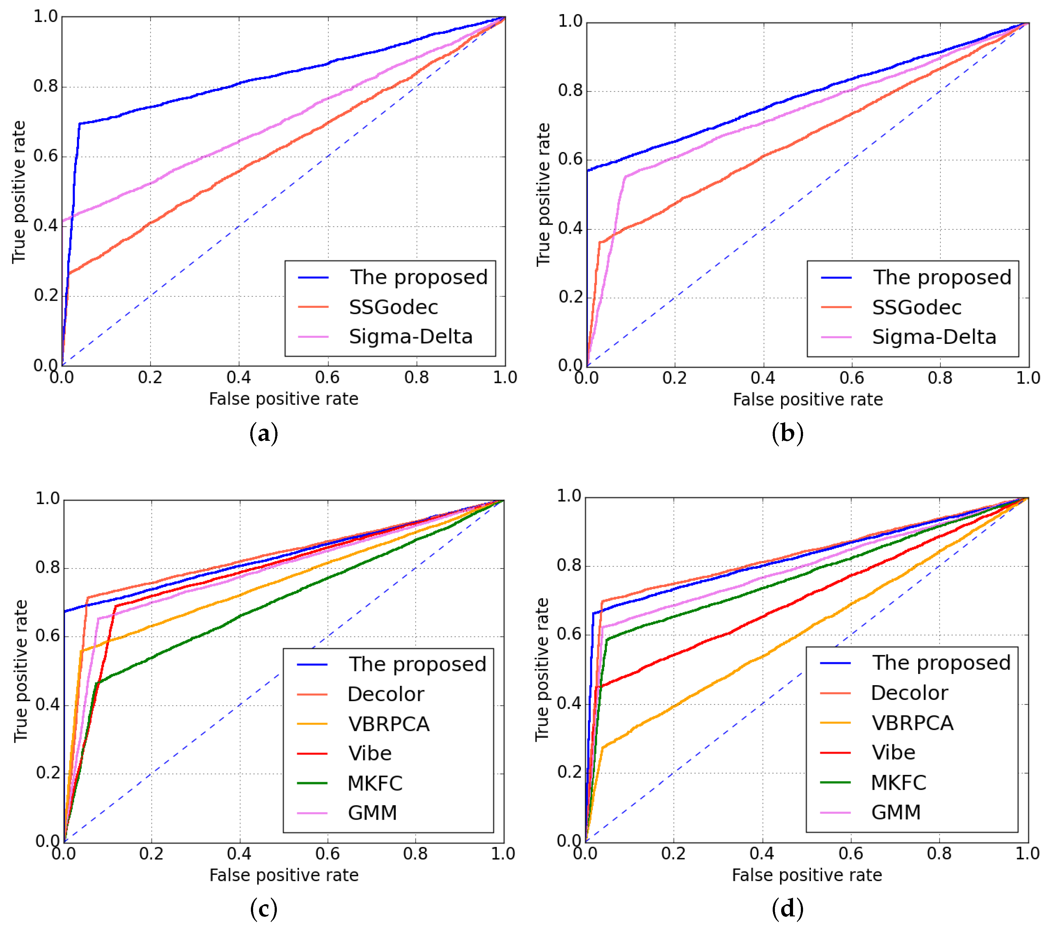
3.1.2. Visual Comparisons on CDNet Dataset

In this sub-experiment, the performance of our method is evaluated by using five video clips from the change detection data set (CDNet) [61]. These clips contain: Shade (periodic motion, shadow), Office (slow-moving), Highway (fast-moving) Winter (camouflage), and Canoe (dynamic background). They are displayed from top to bottom in Figure 10. Seven methods are included for visual comparisons, and they are classified into several categories: (1) Matrix completion approaches: Decolor [67], PCP [22], GROUSE [27]; (2) Probabilistic modeling: GMM [21], VBRPCA [26]; (3) Background modeling: Vibe [34], MKFC [38]. For fast-moving and slow-moving clips, all of these methods are able to reveal ROI details (moving objects) while some noise pixels especially in PCP [22] and GROUSE [27]. When it faces to the shadow or dynamic background source, most of these methods fail because it is hard to handle backgrounds with varying ambient variations. The proposed method shows better results since it ignores ambient variations by object filtering. When processing some sequences like Winter, the proposed method fades in ROI details a little bit since the target contains too small pixels for $\mathcal{M}$ to retrieve, but it still meet a satisfactory result compared with other approaches.

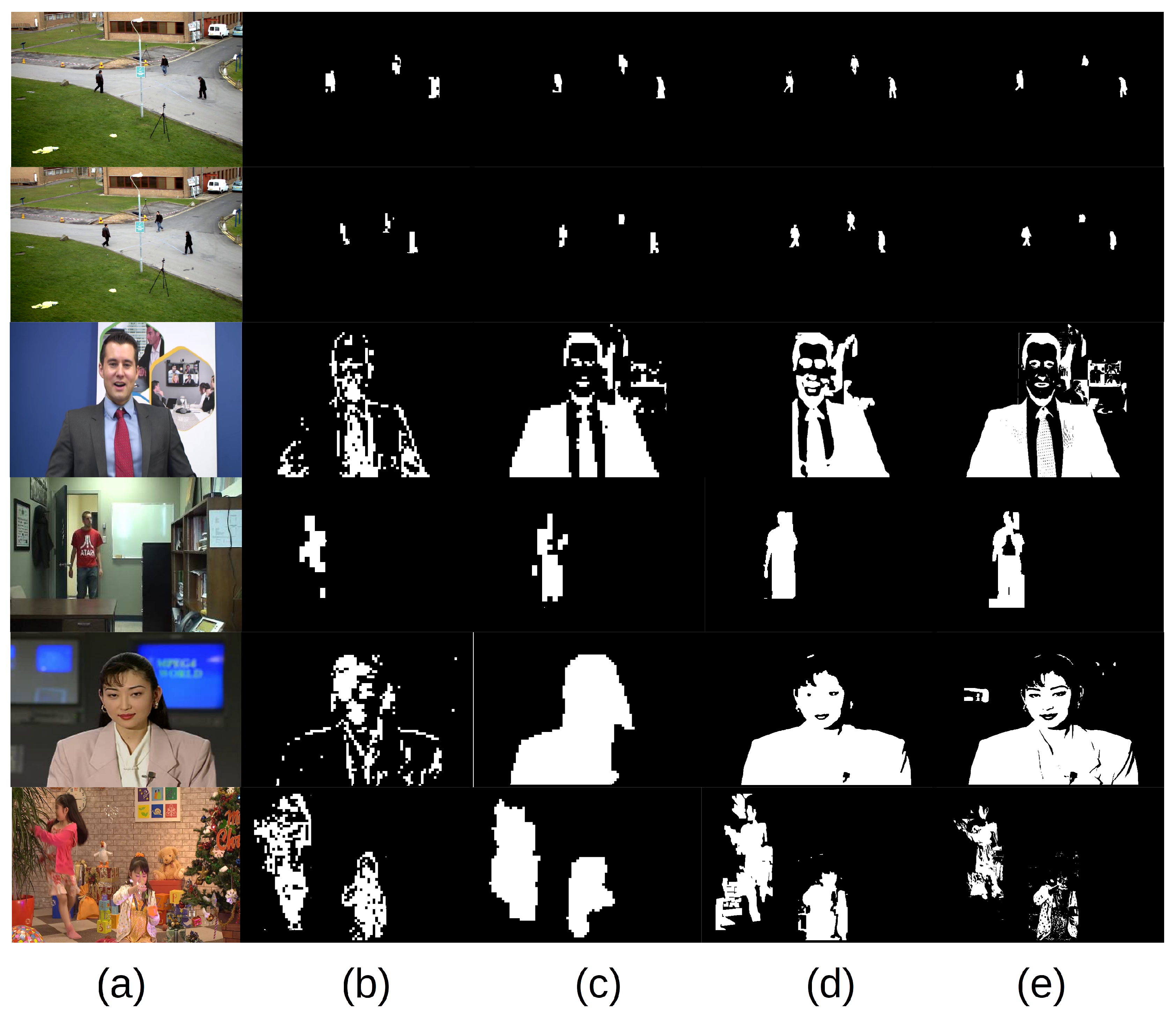
3.1.3. Visual Comparisons On AVC/HEVC Sequences

In this sub-experiment, we test the proposed method among real AVC/HEVC (H.264/H.265) video sample sequences by comparing with other approaches. All the methods are performed based on the standard video compression software named HM13.0 for HEVC. The tested sequence are introduced with a raster order in Figure 11a correspondingly: BQSquare (zooming, slowly move), Carphone (dynamic background), Container (slowly and fast move), Ice (low-contrast fore-background move), KristenAndSara (slowly high definition move), Mobile (zooming, low-contrast fore-background move), Racehorse (large ROI fast move), Stefan (panning, fast move). For comparison purpose, two well-suited for real-time processing embedded in video codec methods are introduced. They are SSGoDec [29] and $\Sigma -\Delta$ motion detection [68], where the former uses outlier pursuit (OP) for low-rank matrix estimation while the latter consists a simple non-linear recursive approximation for background image based on an elementary increment/decrement value. The visual effect result is displayed in Figure 11, where the motion vector output $\mathcal{M}$ (represented as blocks) is displayed in Figure 11b after global motion detection and compensation. One can see that the proposed method achieves better performance especially on sequences with global motion (i.e., Mobile, Stefan) than others. $\Sigma -\Delta$ can extract an explicit margin details specifically in low-contrast fore-background sequences (i.e., Ice), however, it also brings stable details such as the barricades. Our method is able to provide similar object details as $\Sigma -\Delta$ and it also focuses on moving objects with stable details neglected. Similar result can be found in Racehorse.

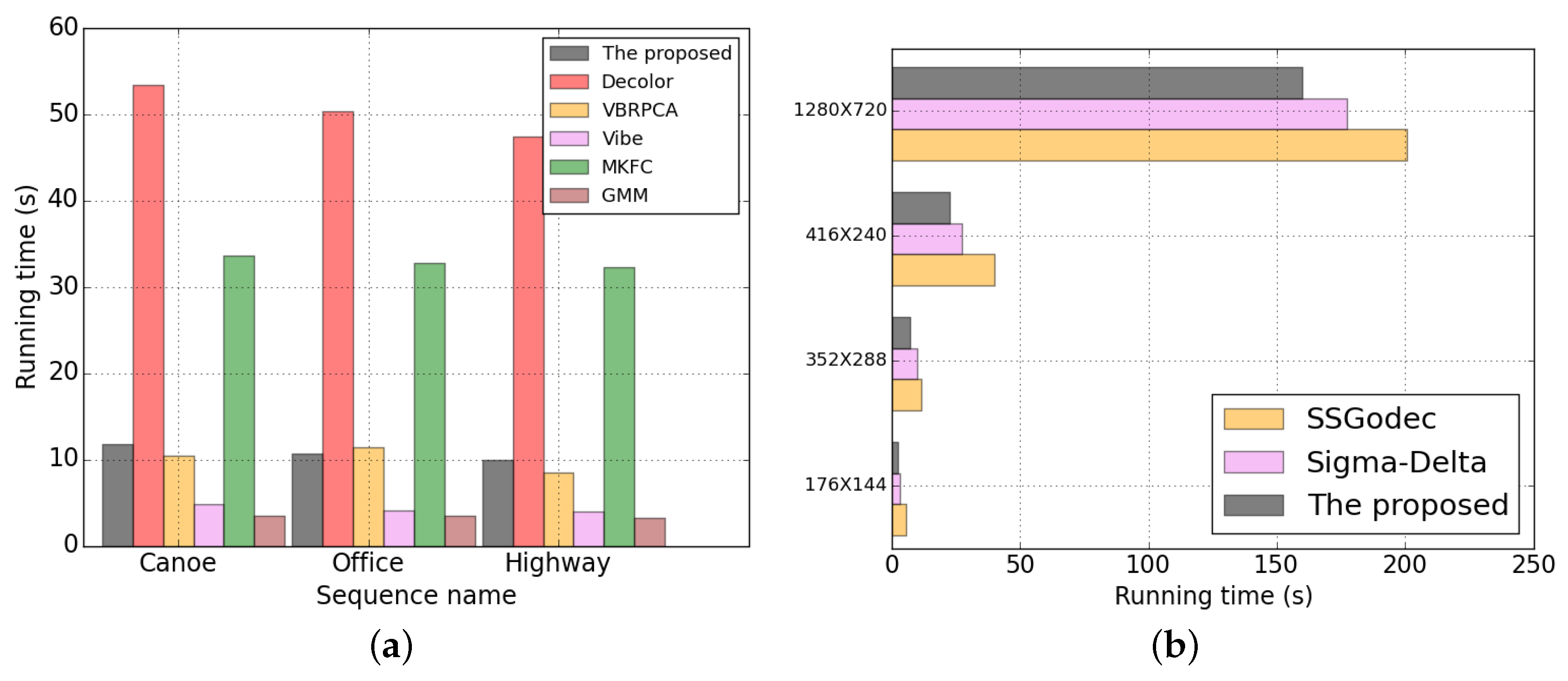
3.1.4. Miscellaneous Analysis

The performance of ROI detection and the computing time for different approaches are analyzed in this sub-experiment. A state-of-the-art measurement for the performance analysis is to plot the ROC curve and compute the area under the curve (AUC). The collected data for test includes the ROI data (white pixels) of the ground truth together with the same amount of the non-ROI data (black pixels), to make sure that we have the same positive and negative samples. The label of classifier is marked as 1 if it belongs to ROI and 0 if not. Unfamiliar with visual effect comparisons, the outputs $I_O$ of these detection methods are gray-scale image (0-255) without binarization by threshold $th$, and the tested data is sorted by a score metric $\widehat{s}(x)$ in a descend order. Also, this sub-experiment addressed some performance metrics analyzes including recall, false positive rate (FPR), false negative rate (FNR), precision (Prec), and F-measure, whose definitions are given by:

$$\left\{\begin{array}{cc}\mathrm{Recall}\hfill & =\mathrm{tp}/(\mathrm{tp}+\mathrm{fn});\mathrm{Prec}=\mathrm{tp}/(\mathrm{fp}+\mathrm{tp});\hfill \\ \mathrm{FNR}\hfill & =\mathrm{fn}/(\mathrm{fn}+\mathrm{tp});\mathrm{FPR}=\mathrm{fp}/(\mathrm{fp}+\mathrm{tn});\hfill \\ \mathrm{F}\text{-}\mathrm{measure}\hfill & =(2\times \mathrm{Recall}\times \mathrm{Prec})/(\mathrm{Recall}+\mathrm{Prec})\hfill \end{array}\right.$$

(24)

where tp, fp, tn, fn denote true positive, false positive, true negative, false negative rate respectively. To begin ROC analysis, we define set $Te$ as the set of test examples (detection outputs); $T{e}^{+}$ and $T{e}^{-}$ are the positive (foreground) and negative (background) subsets, respectively, of $Te$. Meanwhile, a score function, $\widehat{s}(x)$, denotes the score function of the sample pixel x. Then, the ranking accuracy is defined as:

$$rank-acc=\frac{{\displaystyle \sum _{x\in T{e}^{+},x^{\prime }\in T{e}^{+}}}\delta (\widehat{s}(x)>\widehat{s}(x^{\prime }))+\frac{1}{2}\delta (\widehat{s}(x)=\widehat{s}(x^{\prime }))}{Pos·Neg},$$

(25)

where $\delta (·)$ is the indicator function, and $Pos$ and $Neg$ are the number of positive and negative samples, respectively, in $Te$. For convenience, the output image data of each detection method are normalized between 0 and 1 and binarized via a threshold $\xi$, and the score function $\widehat{s}(x)$ is defined as:

$$\widehat{s}(x)=\left\{\begin{array}{c}{(I_g(x)-\xi )}^2,I_g(x)>\xi \hfill \\ -{(I_g(x)-\xi )}^2,I_g(x)<\xi .\hfill \end{array}\right.$$

(26)

Figure 12a,b provide the ROC curve for AVC/HEVC dataset sequences with three detecting methods, and Figure 12a,b stand for CDNet dataset sequences with six detecting methods. One can see that the proposed method has a larger AUC value. In other words, the demand of detection precision for foreground/background classification is reached.

For computation time analysis, we test the performance of each detection method both on CDNet and on AVC/HEVC Sequences. As for CDNet dataset, three sequences (Canoe, Office, Highway) are selected, and each sequence has separated in batches by 20 frames. Figure 13 shows the average batch-running time for these detection methods tested on CDNet dataset. For AVC/HEVC dataset, four different resolutions of sequences are chosen, which are: Container (QCIF), Ice (CIF), Racehorse (416 × 240), KristenAndSara (1280 × 720). Figure 13a displays the time consumption data for different sequences while Figure 13b provides the time consumption data for sequences differ from data resolutions. We can find that the proposed method achieves a lower computation time and better performance on detection precision compared with other approaches. Also, the proposed method intends to find a balance between time costs and detection accuracy.

3.1.5. Performance Comparisons with Motion Vector Extraction Methods

In this subsection, we add some extra experiments that evaluate the performance compared with some other motion vector extraction methods. Based on the authors’ acknowledgements, previous works have introduced the idea of extracting motion vectors of moving objects as ROI detection methods. For example, in [69,70], the authors proposed a two-stage method to identificate moving objects. At the first stage, moving objects are detected based on the analysis of motion vectors in predicted MBs and DCT coefficients in intra-coded MBs. Then, the authors proposed motion vector informations such as spatial correlation, temporal correlation to identify moving objects. Also, they considered the solutions for objects with intra-coded MBs. Niu et al. [71] presented a novel segmentation approach to extract moving objects in the H.264 compressed domain, in which motion vectors are first refined by the motion relativity in both space and time, then clustered based on their differences with the reference of global motion vector. Similarly, work [72] used Global Motion Compensation (GMC) to effectively extract moving objects based on motion vectors. The authors proposed a search-matching algorithm to compute the background motion vectors for global motion extraction. Then, foreground moving objects are identified by excluding global motion vectors. They also introduced a statistic variable named fourth-order moment to distinguish the background signal and moving objects. Recently, Serhan et al. [73] propose a hybrid tracking method which detects moving objects in videos compressed according to H.265/HEVC standard. They introduced Markov Random Field (MRF) model to captures spatial and temporal coherence of the moving object. Also, background/foreground color modeling is proposed both for I frames and for P frames.

Figure 14 displays some visual effects comparisons among those previous works corresponding with motion vector extraction methods. we have selected five sequences for performance tests. These sequences contain both big or small objects (people) with various background changes. Three methods are introduced for comparison purposes; they are Yokoyama et al. [69], Shun et al. [72] and Serhan et al. [73]. As seen in Figure 14, the proposed method meets a satiable results that clearly reflects the details of the moving objects. For detection accuracy analysis, we plot the presion curves among the four tested methods. This results are displayed in Figure 15, one can see that the proposed method can meet the robustness demands for different test cases. Also, the detection precison is more stable than others among the selected test sequences.

4. Conclusions

In this paper, we design a new foreground ROI detection method for video sequences based on two ROI models: “inter” and “intra”. The “inter” model is in charge of acquiring the real motion blocks via global motion detection and compensation. Several detection metrics and a decision tree model are proposed in the inter model, including camera status decision, motion vector subtraction. Also, different categories of camera statuses are taken into consideration with company of global motion compensation. The “intra” model is in charge of revealing the object details by the object filtering approach, and it extracts both the edge and inner part of objects in the frame. Notice that ROI detection focuses on moving details of objects. The output of the “inter” model gives the motion information however not specific which is represented as blocks, while the “intra” model uses this motion information as the pilot and it reconstructs the output by image segmentation and combination using the proposed cluster approach together with a motion area pruning algorithm. Experimental results demonstrate that the proposed method gets a better result both on detection precision and on computational time. Future works will include machine learning approaches to detect the actions of ROI objects and improves the detection quality specifically in the action areas, and the parameters of the proposed method will be optimized which suits video with various characteristics.

References

- Faugeras, O.D. Digital color image processing within the framework of a human visual model. IEEE Trans. Acoust. Speech Signal Process. 1979, 27, 380–393. [Google Scholar] [CrossRef]
- Song, H.; Kuo, C.C. A region-based H.263+ codec and its rate control for low VBR video. IEEE Trans. Multimed. 2004, 6, 489–500. [Google Scholar] [CrossRef]
- Tong, L.; Rao, K. Region of interest based H.263 compatible codec and its rate control for low bit rate video conferencing. In Proceedings of the 2005 International Symposium on Intelligent Signal Processing and Communication Systems, Hong Kong, China, 13–16 December 2005; pp. 249–252. [Google Scholar] [CrossRef]
- Mukherjee, D.; Bankoski, J.; Grange, A.; Han, J.; Koleszar, J.; Wilkins, P.; Xu, Y.; Bultje, R. The latest open-source video codec VP9 - An overview and preliminary results. In Proceedings of the Picture Coding Symposium (PCS), San Jose, CA, USA, 8–11 December 2013; pp. 390–393. [Google Scholar] [CrossRef]
- Sullivan, G.; Ohm, J.; Han, W.J.; Wiegand, T. Overview of the High Efficiency Video Coding (HEVC) Standard. IEEE Trans. Circuits Syst. Video Technol. 2012, 22, 1649–1668. [Google Scholar] [CrossRef]
- Wang, H.; Chang, S.F. A highly efficient system for automatic face region detection in MPEG video. IEEE Trans. Circuits Syst. Video Technol. 1997, 7, 615–628. [Google Scholar] [CrossRef]
- Hartung, J.; Jacquin, A.; Pawlyk, J.; Rosenberg, J.; Okada, H.; Crouch, P. Object-oriented H.263 compatible video coding platform for conferencing applications. IEEE J. Sel. Areas Commun. 1998, 16, 42–55. [Google Scholar] [CrossRef]
- Doulamis, N.; Doulamis, A.; Kalogeras, D.; Kollias, S. Low bit-rate coding of image sequences using adaptive regions of interest. IEEE Trans. Circuits Syst. Video Technol. 1998, 8, 928–934. [Google Scholar] [CrossRef]
- Lam, C.F.; Lee, M. Video segmentation using color difference histogram. In Multimedia Information Analysis and Retrieval, Proceedings of the IAPR International Workshop, MINAR’ 98, Hong Kong, China, 13–14 August 1998; Springer: Berlin/Heidelberg, Germany, 1998; pp. 159–174. [Google Scholar] [CrossRef]
- Schafer, R. MPEG-4: A multimedia compression standard for interactive applications and services. Electron. Commun. Eng. J. 1998, 10, 253–262. [Google Scholar] [CrossRef]
- Zhou, X.; Yang, C.; Zhao, H.; Yu, W. Low-Rank Modeling and Its Applications in Image Analysis. CoRR 2014, arXiv:1401.3409. [Google Scholar] [CrossRef]
- Gupta, S.; Davidson, J.; Levine, S.; Sukthankar, R.; Malik, J. Cognitive Mapping and Planning for Visual Navigation. In Proceedings of the 2017 IEEE Conference on Computer Vision and Pattern Recognition (CVPR), Honolulu, HI, USA, 21–26 July 2017. [Google Scholar]
- Zhang, Z.; Jing, T.; Han, J.; Xu, Y.; Zhang, F. A New Rate Control Scheme For Video Coding Based On Region Of Interest. IEEE Access 2017, 5, 13677–13688. [Google Scholar] [CrossRef]
- Zhang, Z.; Jing, T.; Han, J.; Xu, Y.; Li, X. Flow-Process Foreground Region of Interest Detection Method for Video Codecs. IEEE Access 2017, 5, 16263–16276. [Google Scholar] [CrossRef]
- Zhang, Z.; Jing, T.; Han, J.; Xu, Y.; Li, X.; Gao, M. ROI-Based Video Transmission in Heterogeneous Wireless Networks With Multi-Homed Terminals. IEEE Access 2017, 5, 26328–26339. [Google Scholar] [CrossRef]
- Gonzalez, D.; Botella, G.; Meyer-Baese, U.; Garcia, C.; Sanz, C.; Prieto-Matas, M.; Tirado, F. A low cost matching motion estimation sensor based on the NIOS II microprocessor. Sensors 2012, 12, 13126–13149. [Google Scholar] [CrossRef] [PubMed]
- Gonzalez, D.; Botella, G.; Garcia, C.; Prieto, M.; Tirado, F. Acceleration of block-matching algorithms using a custom instruction-based paradigm on a Nios II microprocessor. EURASIP J. Adv. Signal Process. 2013, 2013, 118. [Google Scholar] [CrossRef]
- Nunez-Yanez, J.L.; Nabina, A.; Hung, E.; Vafiadis, G. Cogeneration of Fast Motion Estimation Processors and Algorithms for Advanced Video Coding. IEEE Trans. Very Large Scale Integr. (VLSI) Syst. 2012, 20, 437–448. [Google Scholar] [CrossRef]
- Stauffer, C.; Grimson, W.E.L. Adaptive background mixture models for real-time tracking. In Proceedings of the 1999 IEEE Computer Society Conference on Computer Vision and Pattern Recognition (Cat. No PR00149), Fort Collins, CO, USA, 23–25 June 1999; Volume 2, p. 252. [Google Scholar] [CrossRef]
- Stauffer, C.; Grimson, W.E.L. Learning Patterns of Activity Using Real-Time Tracking. IEEE Trans. Pattern Anal. Mach. Intell. 2000, 22, 747–757. [Google Scholar] [CrossRef]
- Zivkovic, Z. Improved adaptive Gaussian mixture model for background subtraction. In Proceedings of the 17th International Conference on Pattern Recognition, Cambridge, UK, 26–26 August 2004; Volume 2, pp. 28–31. [Google Scholar] [CrossRef]
- Cand, E.; Li, X.; Ma, Y.; Wright, J. Robust principal component analysis?: Recovering low-rank matrices from sparse errors. In Proceedings of the 2010 IEEE Sensor Array and Multichannel Signal Processing Workshop, Jerusalem, Israel, 4–7 October 2010; pp. 201–204. [Google Scholar] [CrossRef]
- Gao, Z.; Cheong, L.F.; Wang, Y.X. Block-Sparse RPCA for Salient Motion Detection. IEEE Trans. Pattern Anal. Mach. Intell. 2014, 36, 1975–1987. [Google Scholar] [CrossRef] [PubMed]
- Guyon, C.; Bouwmans, T.; Zahzah, E.H. Foreground detection based on low-rank and block-sparse matrix decomposition. In Proceedings of the 2012 19th IEEE International Conference on Image Processing (ICIP), Orlando, FL, USA, 30 September–3 October 2012; pp. 1225–1228. [Google Scholar] [CrossRef]
- Xu, H.; Caramanis, C.; Sanghavi, S. Robust PCA via Outlier Pursuit. IEEE Trans. Inf. Theory 2012, 58, 3047–3064. [Google Scholar] [CrossRef]
- Derin Babacan, S.; Luessi, M.; Molina, R.; Katsaggelos, A.K. Sparse Bayesian Methods for Low-Rank Matrix Estimation. IEEE Trans. Signal Process. 2012, 60, 3964–3977. [Google Scholar] [CrossRef]
- Balzano, L.; Nowak, R.; Recht, B. Online identification and tracking of subspaces from highly incomplete information. In Proceedings of the 2010 48th Annual Allerton Conference on Communication, Control, and Computing (Allerton), Monticello, VA, USA, 29 September–1 October 2010; pp. 704–711. [Google Scholar] [CrossRef]
- Peng, Y.; Ganesh, A.; Wright, J.; Xu, W.; Ma, Y. RASL: Robust Alignment by Sparse and Low-Rank Decomposition for Linearly Correlated Images. IEEE Trans. Pattern Anal. Mach. Intell. 2012, 34, 2233–2246. [Google Scholar] [CrossRef]
- Zhou, T.; Tao, D. GoDec: Randomized Low-rank and Sparse Matrix Decomposition in Noisy Case. In Proceedings of the 28th ICML, Bellevue, WA, USA, 28 June–2 July 2011; pp. 33–40. [Google Scholar]
- Chan, A.B.; Vasconcelos, N. Layered Dynamic Textures. IEEE Trans. Pattern Anal. Mach. Intell. 2009, 31, 1862–1879. [Google Scholar] [CrossRef]
- Chan, A.B.; Vasconcelos, N. Modeling, Clustering, and Segmenting Video with Mixtures of Dynamic Textures. IEEE Trans. Pattern Anal. Mach. Intell. 2008, 30, 909–926. [Google Scholar] [CrossRef] [PubMed]
- Mumtaz, A.; Coviello, E.; Lanckriet, G.R.G.; Chan, A.B. Clustering Dynamic Textures with the Hierarchical EM Algorithm for Modeling Video. IEEE Trans. Pattern Anal. Mach. Intell. 2013, 35, 1606–1621. [Google Scholar] [CrossRef]
- Chan, A.B.; Mahadevan, V.; Vasconcelos, N. Generalized Stauffer–Grimson background subtraction for dynamic scenes. Mach. Vis. Appl. 2011, 22, 751–766. [Google Scholar] [CrossRef]
- Barnich, O.; Droogenbroeck, M.V. ViBe: A Universal Background Subtraction Algorithm for Video Sequences. IEEE Trans. Image Process. 2011, 20, 1709–1724. [Google Scholar] [CrossRef] [PubMed]
- Yao, J.; Odobez, J.M. Multi-Layer Background Subtraction Based on Color and Texture. In Proceedings of the 2007 IEEE Conference on Computer Vision and Pattern Recognition, Minneapolis, MN, USA, 17–22 June 2007; pp. 1–8. [Google Scholar] [CrossRef]
- Maddalena, L.; Petrosino, A. A Self-Organizing Approach to Background Subtraction for Visual Surveillance Applications. IEEE Trans. Image Process. 2008, 17, 1168–1177. [Google Scholar] [CrossRef] [PubMed]
- Panda, D.K.; Meher, S. Detection of Moving Objects Using Fuzzy Color Difference Histogram Based Background Subtraction. IEEE Signal Process. Lett. 2016, 23, 45–49. [Google Scholar] [CrossRef]
- Chiranjeevi, P.; Sengupta, S. Detection of Moving Objects Using Multi-channel Kernel Fuzzy Correlogram Based Background Subtraction. IEEE Trans. Cybern. 2014, 44, 870–881. [Google Scholar] [CrossRef]
- Boykov, Y.; Veksler, O.; Zabih, R. Fast approximate energy minimization via graph cuts. IEEE Trans. Pattern Anal. Mach. Intell. 2001, 23, 1222–1239. [Google Scholar] [CrossRef]
- Kolmogorov, V.; Zabin, R. What energy functions can be minimized via graph cuts? IEEE Trans. Pattern Anal. Mach. Intell. 2004, 26, 147–159. [Google Scholar] [CrossRef]
- Boykov, Y.; Kolmogorov, V. An experimental comparison of min-cut/max- flow algorithms for energy minimization in vision. IEEE Trans. Pattern Anal. Mach. Intell. 2004, 26, 1124–1137. [Google Scholar] [CrossRef]
- Tang, M.; Gorelick, L.; Veksler, O.; Boykov, Y. GrabCut in One Cut. In Proceedings of the 2013 IEEE International Conference on Computer Vision, Sydney, Australia, 1–8 December 2013; pp. 1769–1776. [Google Scholar] [CrossRef]
- He, K.; Zhang, X.; Ren, S.; Sun, J. Spatial Pyramid Pooling in Deep Convolutional Networks for Visual Recognition. In Proceedings of the European Conference on Computer Vision, Zurich, Switzerland, 6–12 September 2014; pp. 346–361. [Google Scholar]
- Szegedy, C.; Toshev, A.; Erhan, D. Deep Neural Networks for Object Detection. Adv. Neural Inf. Process. Syst. 2013, 26, 2553–2561. [Google Scholar]
- Erhan, D.; Szegedy, C.; Toshev, A.; Anguelov, D. Scalable Object Detection Using Deep Neural Networks. In Proceedings of the IEEE Conference on Computer Vision and Pattern Recognition, Columbus, OH, USA, 24–27 June 2014; pp. 2155–2162. [Google Scholar]
- Szegedy, C.; Reed, S.E.; Erhan, D.; Anguelov, D. Scalable, High-Quality Object Detection. CoRR 2014, arXiv:1412.1441. [Google Scholar]
- Ren, S.; He, K.; Girshick, R.B.; Sun, J. Faster R-CNN: Towards Real-Time Object Detection with Region Proposal Networks. CoRR 2015, arXiv:1506.01497. [Google Scholar] [CrossRef] [PubMed]
- He, K.; Zhang, X.; Ren, S.; Sun, J. Spatial Pyramid Pooling in Deep Convolutional Networks for Visual Recognition. IEEE Trans. Pattern Anal. Mach. Intell. 2015, 37, 1904–1916. [Google Scholar] [CrossRef] [PubMed]
- Redmon, J.; Farhadi, A. YOLOv3: An Incremental Improvement. arXiv 2018, arXiv:1804.02767. [Google Scholar]
- Liu, W.; Anguelov, D.; Erhan, D.; Szegedy, C.; Reed, S.E.; Fu, C.; Berg, A.C. SSD: Single Shot MultiBox Detector. CoRR 2015, arXiv:1512.02325. [Google Scholar]
- Huang, G.; Liu, Z.; Weinberger, K.Q. Densely Connected Convolutional Networks. CoRR 2016, arXiv:1608.06993. [Google Scholar]
- Dai, J.; Li, Y.; He, K.; Sun, J. R-FCN: Object Detection via Region-based Fully Convolutional Networks. CoRR 2016, arXiv:1605.06409. [Google Scholar]
- Pinheiro, P.H.O.; Collobert, R.; Dollár, P. Learning to Segment Object Candidates. CoRR 2015, arXiv:1506.06204. [Google Scholar]
- Girshick, R.B.; Donahue, J.; Darrell, T.; Malik, J. Rich feature hierarchies for accurate object detection and semantic segmentation. CoRR 2013, arXiv:1311.2524. [Google Scholar]
- Yuan, J.; Wu, Y. Mining visual collocation patterns via self-supervised subspace learning. IEEE Trans. Syst. Man Cybern. Part B Cybern. 2012, 42, 334–346. [Google Scholar] [CrossRef] [PubMed]
- Zhang, Z.; Jing, T.; Tian, C.; Cui, P.; Li, X.; Gao, M. Objects Discovery Based on Co-Occurrence Word Model with Anchor-Box Polishing. IEEE Trans. Circuits Syst. Video Technol. 2019. [Google Scholar] [CrossRef]
- Chen, Y.M.; Bajic, I.V. A Joint Approach to Global Motion Estimation and Motion Segmentation From a Coarsely Sampled Motion Vector Field. IEEE Trans. Circuits Syst. Video Technol. 2011, 21, 1316–1328. [Google Scholar] [CrossRef]
- Unger, M.; Asbach, M.; Hosten, P. Enhanced background subtraction using global motion compensation and mosaicing. In Proceedings of the 2008 15th IEEE International Conference on Image Processing, San Diego, CA, USA, 12–15 October 2008; pp. 2708–2711. [Google Scholar] [CrossRef]
- Jin, Y.; Tao, L.; Di, H.; Rao, N.I.; Xu, G. Background modeling from a free-moving camera by Multi-Layer Homography Algorithm. In Proceedings of the 2008 15th IEEE International Conference on Image Processing, San Diego, CA, USA, 12–15 October 2008; pp. 1572–1575. [Google Scholar] [CrossRef]
- Guerreiro, R.F.C.; Aguiar, P.M.Q. Global Motion Estimation: Feature-Based, Featureless, or Both?! In Image Analysis and Recognition, Proceedings of the Third International Conference, ICIAR 2006, voa de Varzim, Portugal, 18–20 September 2006; Springer: Berlin/Heidelberg, Germany, 2006; pp. 721–730. [Google Scholar]
- The Change Detection Dataset. Available online: http://changedetection.net (accessed on 25 March 2019).
- The HEVC/AVC Official Test Sequences, Online. Available online: ftp://hevc@ftp.tnt.uni-hannover.de/testsequences (accessed on 25 March 2019).
- Su, Y.; Sun, M.T.; Hsu, V. Global motion estimation from coarsely sampled motion vector field and the applications. IEEE Trans. Circuits Syst. Video Technol. 2005, 15, 232–242. [Google Scholar] [CrossRef]
- Smolic, A.; Hoeynck, M.; Ohm, J.R. Low-complexity global motion estimation from P-frame motion vectors for MPEG-7 applications. In Proceedings of the 2000 International Conference on Image Processing (Cat. No.00CH37101), Vancouver, BC, Canada, 10–13 September 2000; Volume 2, pp. 271–274. [Google Scholar] [CrossRef]
- Fischler, M.A.; Bolles, R.C. Random Sample Consensus: A Paradigm for Model Fitting with Applications to Image Analysis and Automated Cartography. In Readings in Computer Vision: Issues, Problems, Principles, and Paradigms; Morgan Kaufmann Publishers Inc.: San Francisco, CA, USA, 1987; pp. 726–740. [Google Scholar] [CrossRef]
- Jarvis, R. On the identification of the convex hull of a finite set of points in the plane. Inf. Process. Lett. 1973, 2, 18–21. [Google Scholar] [CrossRef]
- Zhou, X.; Yang, C.; Yu, W. Moving Object Detection by Detecting Contiguous Outliers in the Low-Rank Representation. IEEE Trans. Pattern Anal. Mach. Intell. 2013, 35, 597–610. [Google Scholar] [CrossRef] [PubMed]
- Rueda, L.; Mery, D.; Kittler, J. Σ-Δ Background Subtraction and the Zipf Law. In Progress in Pattern Recognition, Image Analysis and Applications, Proceedings of the 12th Iberoamericann Congress on Pattern Recognition, CIARP 2007, Valparaiso, Chile, 13–16 November 2007; Springer: Berlin/Heidelberg, Germany, 2007; pp. 42–51. [Google Scholar] [CrossRef]
- Yokoyama, T.; Iwasaki, T.; Watanabe, T. Motion Vector Based Moving Object Detection and Tracking in the MPEG Compressed Domain. In Proceedings of the 2009 Seventh International Workshop on Content-Based Multimedia Indexing, Chania, Greece, 3–5 June 2009; pp. 201–206. [Google Scholar] [CrossRef]
- Yoneyama, A.; Nakajima, Y.; Yanagihara, H.; Sugano, M. Moving object detection and identification from MPEG coded data. In Proceedings of the 1999 International Conference on Image Processing (Cat. 99CH36348), Kobe, Japan, 24–28 October 1999; Volume 2, pp. 934–938. [Google Scholar] [CrossRef]
- Niu, C.; Liu, Y. Moving Object Segmentation Based on Video Coding Information in H.264 Compressed Domain. In Proceedings of the 2009 2nd International Congress on Image and Signal Processing, Tianjin, China, 17–19 October 2009; pp. 1–5. [Google Scholar] [CrossRef]
- Zhang, S.; Su, X.; Xie, L. Global motion compensation for image sequences and motion object detection. In Proceedings of the 2010 International Conference on Computer Application and System Modeling (ICCASM 2010), Taiyuan, China, 22–24 October 2010; Volume 1, pp. V1–406–V1–409. [Google Scholar] [CrossRef]
- Gul, S.; Meyer, J.T.; Hellge, C.; Schierl, T.; Samek, W. Hybrid video object tracking in H.265/HEVC video streams. In Proceedings of the 2016 IEEE 18th International Workshop on Multimedia Signal Processing (MMSP), Montreal, QC, Canada, 21–23 September 2016; pp. 1–5. [Google Scholar] [CrossRef]