Article

Path Planning for Multi-UAV Formation Rendezvous Based on Distributed Cooperative Particle Swarm Optimization

1
School of Aeronautics, Northwestern Polytechnical University, Xi’an 710072, China
2
School of Astronautics, Northwestern Polytechnical University, Xi’an 710072, China
3
UAV Research Institute, Northwestern Polytechnical University, Xi’an 710065, China
*
Author to whom correspondence should be addressed.
Appl. Sci. 2019, 9(13), 2621; https://doi.org/10.3390/app9132621
Submission received: 4 June 2019 / Revised: 25 June 2019 / Accepted: 27 June 2019 / Published: 28 June 2019
(This article belongs to the Special Issue Unmanned Aerial Vehicles (UAVs))

Abstract

:

Featured Application

The cooperative path planning problem of multi-UAV is becoming more and more important. The proposed path-planning algorithm presented in this paper can be used in some formation rendezvous applications, such as formation reconnaissance and attack.

Abstract

This paper studies the problem of generating cooperative feasible paths for formation rendezvous of unmanned aerial vehicles (UAVs). Cooperative path-planning for multi-UAV formation rendezvous is mostly a complicated multi-objective optimization problem with many coupled constraints. In order to satisfy the kinematic constraints, i.e., the maximum curvature constraint and the requirement of continuous curvature of the UAV path, the Pythagorean hodograph (PH) curve is adopted as the parameterized path because of its curvature continuity and rational intrinsic properties. Inspired by the co-evolutionary theory, a distributed cooperative particle swarm optimization (DCPSO) algorithm with an elite keeping strategy is proposed to generate a flyable and safe path for each UAV. This proposed algorithm can meet the kinematic constraints of UAVs and the cooperation requirements among UAVs. Meanwhile, the optimal or sub-optimal paths can be obtained. Finally, numerical simulations in 2-D and 3-D environments are conducted to demonstrate the feasibility and stability of the proposed algorithm. Simulation results show that the paths generated by the proposed DCPSO can not only meet the kinematic constraints of UAVs and safety requirements, but also achieve the simultaneous arrival and collision avoidance between UAVs for formation rendezvous. Compared with the cooperative co-evolutionary genetic algorithm (CCGA), the proposed DCPSO has better stability and a higher searching success rate.

1. Introduction

Unmanned aerial vehicles (UAVs) are widely used in both civilian and military fields, including search and rescue [1], environmental monitoring [2], surveillance and attacks [3], and so on. Based on the multi-agent theory and applications [4,5,6], a group of UAVs flying in a formation [7] rather than a single UAV can obtain higher combating effectiveness, deliver greater coverage, and will have wider applications in the future.
Regarding the multi-agent formation problem, some important studies exist. Olfati-Saber described a theoretical framework for the design and analysis of the distributed flocking algorithm for the multi-agent self-organizing flocking problem, two constraint-free algorithms, and one constrained algorithm considering the obstacles proposed. For generating regular polygon formation of a multi-robot, each robot is represented as an electric charge. The formation can be realized based on the attractive forces of a virtual center and the repulsive forces between different robots; the collision avoidance with obstacles can be achieved based on the potential field theory [8,9]. Nguyen et al. [10] propose a distributed formation control algorithm to form different formation shapes for multiple rectangular agents. An artificial potential function is used and a repulsive function is used to avoid collision. To make the UAVs reach a predetermined rendezvous state simultaneously, path-planning for multi-UAV formation rendezvous becomes one of the key technologies in UAV formation flying.
Recently, many researchers have been looking into the problem of cooperative path-planning of multiple UAVs [11,12,13]. To solve the problem of multi-UAV rendezvous, the velocity control method is used [14,15]. Manathara et al. [14] use the consensus algorithm based on the estimated time of arrival, where velocity control and a wandering maneuver are applied to avoid collisions with other UAVs. Unfortunately, this method requires a large amount of communication. Regarding the cooperative timing problem among multiple UAVs, the path and velocity of each UAV are determined by the coordination functions and coordination variable; however, this may lead to velocity saturation [16]. Some other researchers use the trajectory control method [17,18,19] to realize multi-UAV rendezvous, which assumes that each UAV flies at a constant and equal velocity. For multiple UAVs performing many-to-one tasks, two wandering maneuvers [18] based on Dubins curve are proposed to achieve simultaneous arrival. A simple method based on basic geometry [19] is proposed to generate paths of equal length in a remote-sensing problem, where each UAV first calculates the Dubins longest path. Because a Dubins curve consists of arcs of the minimal turning radius and straight lines, the discontinuous curvature of Dubins curve leads to a large tracking error for UAV. A three-step method is proposed [20] to generated feasible UAV paths to achieve simultaneous arrival; the connection of the arc and line in Dubins path is replaced with the clothoid arc. The method consists of (i) generating flyable paths using Dubins path with clothoid arcs, (ii) satisfying the collision avoidance constraint, and (iii) generating paths of equal length. However, this method requires a large amount of computation because of the iteration strategy.
According to the existing literature on cooperative path-planning of UAVs, the commonly used paths are as follows: Dubins paths [14,21], clothoid paths [20,22], B-spline paths [18,23], and Pythagorean hodograph (PH) paths [16,24]. The Dubins path is the shortest path, but it has discontinuous curvature; the other three paths have continuous curvature. Regarding the clothoid path, there is no closed-form solution and iteration is required for a solution. For the B-spline path, the curvature at any point on the curve has no closed-form solution and it is difficult to meet the maximum-curvature constraint of UAVs. The PH path is parameterized by polynomials as a function of the path length and provides closed-form polynomials for path length and curvature. In addition, the position and direction at the initial and final locations are directly considered as boundary conditions, trading off the path length and its curvature to meet the maximum-curvature constraint. In order to take full advantage of the PH path, the PH curve is adopted from other literature as the parameterized path of the UAV in this paper.
In this paper, the focus is on generating a group of cooperative paths for UAVs arriving at the rendezvous point simultaneously and forming a desired formation configuration. A distributed cooperative particle swarm optimization (DCPSO) algorithm with a cooperation mechanism is proposed, which also serves as the contributions of the paper. The PH paths of all UAVs are optimized cooperatively by using the DCPSO algorithm. Using a distributed cooperation mechanism, the particles in each sub-swarm are modified so that the kinematic constraints of UAVs, the collision avoidance, and the simultaneous arrival of the UAV formation are achieved. Meanwhile, the optimal or sub-optimal paths are obtained.
The rest of this study is organized as follows. The multi-UAV formation rendezvous problem formulation is presented in Section 2. Section 3 describes the distributed cooperative particle swarm optimization algorithm for multiple UAVs. Simulation results are shown in Section 4. The summary and conclusions are given in Section 5.

2. Problem Formulation

2.1. Formation Rendezvous of Multi-UAVs

Given the problem of formation rendezvous for N UAVs, suppose the starting pose (position and direction) at initial location of UAV i is given as p s i = ( x s i , y s i , z s i , χ s i , γ s i ) and the formation pose p f = ( x f , y f , z f , χ f , γ f ) at the rendezvous point is also known beforehand, where ( x , y , z ) is the location of UAV or formation and ( χ , γ ) are the horizontal and vertical angles, respectively. The formation configuration at the rendezvous point is defined with the virtual structure approach [25] by a series of relative coordinates { ( x f i , y f i , z f i ) | i = 1 , , N } in the moving frame p f X f Y f Z f , which is attached to the formation center as shown in Figure 1. Therefore, the desired pose p d i = ( x d i , y d i , z d i , χ d i , γ d i ) of UAV i around the rendezvous point can be calculated with coordinate transformation. Path-planning for multi-UAV formation rendezvous involves producing a group of paths r i ( q ) connecting p s i and p d i . Mathematically, this can be represented as:
p s i = ( x s i , y s i , z s i , χ s i , γ s i ) r i ( q ) p d i = ( x d i , y d i , z d i , χ d i , γ d i ) , i = 1 , , N
where r i ( q ) is the resulting path of UAV i , q is defined as a path parameter, and ∐ represents the constraints, including the kinematic constraints of UAVs, safety requirements, simultaneous arrival with other UAVs, and so on. In view of this, all UAVs should have the same speed when formation is achieved at the rendezvous point before entering into the next stage of formation keeping. We assume that all UAVs have the same constant speed during the formation rendezvous for simplicity. Hence, simultaneous arrival can be achieved by generating a group of paths with equal or approximately equal length.
As mentioned, the total cost of all the generated paths should achieve the minimum or second minimum, as well as satisfying a variety of constraints. There are some commonly used criteria for evaluating a UAV path, including fuel consumption, path smoothness, radar threats, and other safety costs, i.e., terrain avoidance, obstacle avoidance, and no-fly zone avoidance. In view of the limited flexibility of a single PH path, the rendezvous environment is supposed to be much simpler than the combat environment, with only a few obstacles and no-fly zones.
Figure 1 shows the schematic of cooperative path planning for a 4-UAV formation rendezvous in the top view. A diamond configuration is defined at the rendezvous point, where O g X g Y g Z g is the inertial frame. No-fly zones are represented by rectangles and obstacles are represented by circles in the 2-D plane and cylinders in the 3-D environment.

2.2. Pythagorean Hodograph Path

The Pythagorean hodograph (PH) curve was first introduced by Farouki and Sakkalis [26] in 1990. It is defined by a parameterized polynomial curve which has hodographs that satisfy a Pythagorean condition. The definition is given as:
Definition 1.
(The PH curve [26]). Suppose that r ( q ) = { x ( q ) , y ( q ) , z ( q ) } is a polynomial curve parameterized by q . r ( q ) is a PH curve, if the first derivatives of its components satisfy the following Pythagorean condition:
x 2 ( q ) + y 2 ( q ) + z 2 ( q ) = σ 2 ( q ) ,
where x ( q ) , y ( q ) , z ( q ) and σ ( q ) are polynomials of q .
In view of numerical stability, PH curves can be written in the following Bernstein–Bézier form [16,26]:
r ( q ) = k = 0 n p k ( n k ) ( 1 q ) n k q k , q [ 0 , 1 ] ,
where p k is known as the “control point” of the curve and n is the order of the curve. According to [27,28], the lowest order of PH curve that has an inflection point is the fifth, called the quintic PH curve. The inflection point provides sufficient flexibility in path shape to be appropriate for path-planning. Hence, the quintic PH curve is applied for UAV path-planning in this paper.
Generally, the poses at the initial and final locations, namely boundary conditions r ( 0 ) , r ( 0 ) , r ( 1 ) and r ( 1 ) , are known beforehand. Then, the first-order Hermite interpolation [29], combined with the complex vector method or with the quaternion method [29], can be used to solve the 2-D or 3-D quintic PH curve. Details about the solving process are introduced in [29,30]. After getting the polynomial expression of the PH path r ( q ) , the path length of the PH curve can be obtained by integrating the polynomial r ( q ) , namely,
L ( q ) = r ( q ) , q [ 0 , 1 ] .
According to differential geometry theory [22], the curvature and torsion are fundamental properties of a curve, by which the smoothness of the curve is completely determined. In 2-D cases, the torsion is identically equal to zero. Curvature describes the bending extent of a curve, while torsion represents the twisting extent. For UAVs, these two properties also play an important role in the mechanics of a vehicle. The curvature is proved proportional to the lateral acceleration, while the torsion is proportional to the angular momentum. Thus, the UAV path should satisfy the maximum-curvature and maximum-torsion constraints, which are known as the kinematic constraints of a UAV. The curvature and torsion at any point on the path can be solved by following equations [22]:
κ ( q ) = | r ( q ) × r ( q ) | | r ( q ) | 3 ,
τ ( q ) = ( r ( q ) × r ( q ) ) r ( q ) | r ( q ) × r ( q ) | 2 ,
where r ( q ) , r ( q ) and r ( q ) are the first, second, and third derivatives of r ( q ) , respectively. Obviously, the curvature and torsion of a PH path are rational polynomials. To describe the smoothness of a PH path quantitatively, we introduce the definition of the elastic energy of a curve.
Definition 2.
(The elastic energy [31]). The elastic energy of a curve is defined as the integral of the sum of squares of curvature and torsion with respect to arc length, namely:
E = ( κ 2 + τ 2 ) d s .
In general, the lengths of direction vectors, m 0 = r ( 0 ) and m 1 = r ( 1 ) , are considered to be the control variables. The lager the values of m 0 and m 1 , the smoother the PH path, but the greater the path length. Therefore, appropriate values of m 0 and m 1 are optimized so that the kinematic constraints of UAVs are satisfied, namely | κ ( q ) | κ max and | τ ( q ) | τ max .

3. DCPSO with Cooperation

As addressed above, cooperative path-planning for multi-UAV formation rendezvous is mostly a complicated multi-objective optimization problem with many coupled constraints. The solutions of the problem are a collection of UAV paths and each UAV path is part of the solution set. The relationship between these two is similar to that between population and subpopulation in the co-evolutionary theory [32]. Inspired by the co-evolutionary theory, cooperative co-evolutionary genetic algorithms (CCGA) have been applied in path-planning for multiple robots or UAVs [33,34]. However, the conventional CCGA has low search efficiency and may easily trap local optimum. The existing cooperative particle swarm optimization (CPSO) [35,36] can easily jump out of local optimum, but they lack effective cooperation between subpopulations and cannot be directly used for path-planning for multiple UAVs. To take full advantage of CPSO, a distributed cooperative particle swarm optimization (DCPSO) algorithm with cooperation is proposed.

3.1. Standard Particle Swarm Optimization (PSO)

Particle swarm optimization (PSO) is a population-based heuristic method. It was first proposed by Elberhart and Kennedy in 1995, who were inspired by the social behavior of bird flocks. The PSO algorithm is widely used in optimal scheduling [37,38], path-planning [11,23], big data digging [39], and so on. PSO owns several evolutionary characteristics similar to genetic algorithms (GA), such as initialization with a population of random solutions and updating based on previous generations. However, PSO has fewer setting parameters, simpler implementation, and a faster convergence rate compared with GA.
A swarm of particles are randomly initialized in the PSO algorithm. Each particle has three properties, which are position, velocity, and fitness. Assuming a swarm of n particles in a D-dimensional optimization problem, the velocity and position of particle i are denoted as V i = ( v i 1 , , v i D ) and X i = ( x i 1 , , x i D ) , respectively. The fitness of particle i can be solved by the fitness function. The best solution of particle i found so far is represented as p best i = ( p i 1 , , p i D ) , generally known as the personal best location and the best position found by all particles so far is denoted as g best = ( g 1 , , g D ) , known as the global best location. In each iteration, each particle’s velocity and position are updated using the following equation:
v i d ( t + 1 ) = ϖ ( t ) v i d ( t ) + c 1 r 1 ( p i d ( t ) x i d ( t ) ) + c 2 r 2 ( g d ( t ) x i d ( t ) )
x i d ( t + 1 ) = x i d ( t ) + v i d ( t + 1 )
where i = 1 , 2 , , n , d = 1 , 2 , , D , t = 1 , 2 , , T , T is the maximum generation number, ϖ is the inertia weigh, c 1 and c 2 are acceleration coefficients which are typically set to c 1 = c 2 = 2 , and r 1 and r 2 are randomly generated within [ 0 , 1 ] , which are used to keep the diversity of the swarm. From Equation (8) we can see that the velocity updating term consists of three parts: ϖ ( t ) v i d ( t ) , which is the inherited velocity from previous generation, reflecting the particle’s memory property; c 1 r 1 ( p i d ( t ) x i d ( t ) ) , which is the cognitive learning velocity from its history, attracting the particle to its historical best position; and c 2 r 2 ( g d ( t ) x i d ( t ) ) , which is the social learning velocity from the swarm history, attracting the particle to the historical best position of the swarm. Generally, for fear of a blind search, the velocity and position of each particle are limited to [ V max , V max ] and [ X min , X max ] .

3.2. Distributed Cooperative Particle Swarm Optimization with Cooperation

The PH path is adopted as the parameterized path of a UAV in this paper. According to the theory of the PH curve, a path is determined by the lengths of direction vectors, namely m 0 and m 1 , under certain poses at initial and final locations. So, the path-planning for N UAV formation rendezvous means getting each UAV a pair of ( m 0 , m 1 ) so that the corresponding PH path can meet those constraints (including safety requirements, kinematic constraints, cooperation requirements, and others) and the total cost of all paths reaches the minimum or second minimum.
Here, the possible solutions of N UAVs are regarded as N sub-swarms or subpopulations. A distributed cooperative particle swarm optimization (DCPSO) with cooperation mechanism is proposed to optimize the N PH paths cooperatively. The particles in each sub-swarm update their positions and velocities and finish their fitness computations independently, which is the same procession as the standard PSO. In order to achieve cooperation within UAVs, each sub-swarm communicates with the others to transmit their representative individuals, then N cooperative groups are formed. Then, in each new-forming group, fitness of particles in the current subpopulation is modified and the personal and group best locations are also modified. Therefore, particles in each sub-swarm will move to the optimal or suboptimal solutions with cooperation between UAVs. The flow chart of the DCPSO with cooperation is given in Figure 2. It can be seen that information interaction between UAVs only happens in forming cooperative groups and fitness modification, which means the proposed algorithm has a distributed structure. To improve searching efficiency, an elite keeping strategy is adopted.

3.2.1. Algorithm Initialization

As addressed, each particle j in sub-swarm i denotes an alternative PH path of UAV i , which is represented as z i j = ( m i j , 0 , m i j , 1 ) . The particle’s velocity is represented as v i j = ( v i j , 0 , v i j , 1 ) , i = 1 , , N , and j = 1 , , M , where M is the sub-swarm’s size. According to the prescribed search space [ Z min , Z max ] and velocity range [ V max , V max ] , all particles’ positions and velocities can be assigned randomly. The particles’ initial fitness is calculated and cooperatively modified in a way that will be introduced in subsequent sections. The personal best locations and group best locations are also initialized.

3.2.2. Update of Velocities and Positions

According to the standard PSO algorithm, the velocity and position of particle z i j can be updated with Equation (8) and Equation (9), respectively. What is more, the value of inertia weight ϖ plays an important role in creating a balance between global exploration and local exploitation. A large value for ϖ facilitates global exploration, which is useful in the initial stages of an optimization. However, a small value allows for better local searching, which is particularly useful in the later stages, as the swarm moves toward the neighborhood of the optimum.
In [40], a value for ϖ dynamically decreasing from 0.9 to 0.4 is recommended for better performance. Hence, a dynamically changed ϖ is adopted in this paper, which is updated by the following equation:
ϖ ( t ) = ϖ s t a r t ( ϖ s t a r t ϖ e n d ) ( t T ) 2 ,
where ϖ s t a r t = 0.9 , ϖ e n d = 0.4 , and T is the maximum number of iterations.

3.2.3. Fitness Function

In order to generate a flyable and safe PH path for UAV i with a short length and appropriate smoothness, the fitness function for UAV i is designed as:
f i = 1 / ( w 1 J i , fuel + ( 1 w 1 ) J i , curve + J i , obsc + J i , nofly + J i , terr + J i , unflyble ) ,
where w 1 is a user-defined weight parameter. J i , fuel is the cost of fuel consumption, which is approximately proportional to the path length of UAV i . Here, let J i , fuel = L i , where path length L i can be calculated by Equation (4). J i , curve is the cost of path smoothness, which can be described by the elastic energy of the PH path. Hence, let J i , curve = E i , where the elastic energy E i is calculated by Equation (7). J i , obsc , J i , nofly , J i , terr , and J i , unflyble are the penalty functions for avoiding the obstacles, no-fly zones, collisions with terrain, and meeting the maximum curvature and torsion constraints, respectively.
For simplicity, the PH path is discretized as N p points. If all the discretized points do not collided with the obstacles or pass through the no-fly zones, J i , obsc = 0 or J i , nofly = 0 ; otherwise, a large positive number (like 10 5 ) is assigned to J i , obsc or J i , nofly . Similarly, if all the discretized points can avoid collision with the terrain, J i , terr = 0 ; otherwise, a large positive number (like 10 5 ) is assigned. If the curvature and torsion at all discretized points satisfy the maximum curvature and torsion constraints, the PH path is considered flyable and J i , unflyble = 0 ; otherwise a large positive number is assigned, which can be formulized as:
J i , unflyble = { 10 5 , max q | κ i ( q ) | > κ max | | max q | τ i ( q ) | > τ max 0 max q | κ i ( q ) | κ max   &   max q | τ i ( q ) | τ max ,
where κ max and τ max are the maximum curvature and torsion, respectively.
In a 3-D environment, the terrain is simulated by following function:
H ( x , y ) = a sin ( x + b ) + c sin ( y + d ) + e cos ( f x 2 + y 2 ) + g sin ( h x + l y ) ,
where a , b , c , d , e , f , g , h , and l are custom constants.

3.2.4. Cooperative Fitness Modification

For achieving the simultaneous arrival and collision avoidance between UAVs, a cooperation mechanism among all the sub-swarms is proposed as follows. After obtaining all the particles’ fitness, each sub-swarm has to offer a representative particle based on their fitness, then N new cooperative groups are formed. Each cooperative group i consists of the sub-swarm i and all the representative particles. Generally, selecting the representative particle for a sub-swarm is very important; the current best particle or the historical best one is usually selected. In this paper, the group best location of each sub-swarm is selected as its representative particle.
Then, the particles in each cooperative group are required to modify their fitness according to all the representative particles. Namely, for cooperative group i , check whether the particles of sub-swarm i will collide with the representatives from other sub-swarms; if collision happens, a penalty term is added to the particle’s fitness. Meanwhile, among the N representatives, find j , which is the one that has the largest path length as the reference particle; its path length is seen as the reference path length L ref . To satisfy the simultaneous arrival constraint of multi-UAV formation, if the reference particle j does not belong to sub-swarm i , namely i j , the particles in sub-swarm i are required to modify their fitness by adding a penalty term. The penalty term is directly proportional to the absolute difference between the path length of a current particle and the reference one. Thus, the larger length difference will obtain the larger penalty value. Therefore, the modified fitness function of particle i is denoted as follows:
f i = 1 / ( 1 / f i + J i , collision + J i , dtime ) ,
where J i , collision and J i , dtime are the added penalty values, which can be expressed as:
J i , collision = { 10 5 , collision 0 collision - free ,
J i , dtime = { 100 | L i L ref | 2 , i j 0 , i = j ,
where L i is the path length of any particle in subpopulation i .
Determining the collision between two UAVs by using the rotational properties of PH path is described in detail as follows. If there is no collision between two PH paths, the minimum separation distance between these two paths should be greater than the sum of the two UAVs’ safety radiuses at any moment.
Consider two PH paths of UAV i and UAV j , namely r i ( q ) and r j ( q ) . Their safety radiuses are represented as R i and R j , respectively. For simplicity, each PH path is discretized as N ph equidistant points. Because all UAVs fly at a same constant speed and arrive at the rendezvous point simultaneously, the distance between the two UAVs at any moment approximately equals the distance between the two equidistant points with the same number. Hence, the minimum separation distance between the two paths approximately equals the minimum distance between any two equidistant points with the same number. As shown in Figure 3, the safety balls are centered on the equidistant points along each path. If the safety balls overlap at any equidistant points with the same number on each path, a collision could happen. According to the rotational properties of PH path, the path length can be calculated by the polynomial Equation (4). Hence, the corresponding path parameter q at any equidistant point along a PH path can be solved by the Newton–Raphson iterative method. The coordinates of each equidistant point are obtained by Equation (3). Supposing the coordinates of any equidistant points k of r i ( q ) and r j ( q ) are represented as ( x i , k , y i , k , z i , k ) and ( x j , k , y j , k , z j , k ) , and k = 1 , , N ph . Therefore, the constraint of collision avoidance between any two UAVs can be written as:
d i s min , i j > R i + R j d i s min , i j = min { d i s i j ( k ) | k = 1 , , N ph } d i s i j ( k ) = ( x i , k x j , k ) 2 + ( y i , k y j , k ) 2 + ( z i , k z j , k ) 2 i j , i = 1 , , N , j = 1 , , N , ,
where d i s min , i j is the minimum separation distance.

3.2.5. Cooperative Path-Planning with DCPSO

In conclusion, the formation rendezvous problem of multi-UAV based on DCPSO can be solved by the following steps:
Step 1. Initialize all sub-swarms:
(1) For the N UAVs, the size of each sub-swarm is M , T is the maximum iteration number, and the current iteration is set to t = 0 ;
(2) The velocities and positions of all the particles are initialized within the bounded search space [ V max , V max ] and [ Z min , Z max ] , respectively;
(3) Each particle’s fitness is calculated using Equation (11); the best particle in each sub-swarm is selected as its representative. Each particle’s fitness is modified cooperatively using Equation (14). Then, the initial personal and global best solutions are easy to obtain.
Step 2. The particles’ velocities and positions in each sub-swarm are updated using Equation (8) and Equation (9), which are limited within the prescribed search space and velocity range. Then, each particle’s fitness is calculated using Equation (11). To improve the searching efficiency of the DCPSO algorithm, an elite keeping method is used. In each sub-swarm, the best particle of the previous generation is used to replace the worst one in the current generation.
Step 3. The group best location of each sub-swarm is selected as the representative and cooperative groups are formed. Then, each particle’s fitness is modified in each cooperation group using Equation (14).
Step 4. For each sub-swarm i, compare every particle z i j with the personal best location p best i j ; if the particle is better, let p best i j = z i j , i = 1 , , N , j = 1 , , M .
Step 5. For each sub-swarm i, compare every particle z i j with the group best location g best i ; if the particle is better, let g best i = z i j , i = 1 , , N , j = 1 , , M .
Step 6. If t = T , end the iteration and output the best solutions of each sub-swarm; otherwise, let t = t + 1 and go back to Step 2.

3.2.6. Time Complexity Analysis and Remarks

The time complexity analysis on the proposed DCPSO algorithm with cooperation is given as follows:
(1) The time complexity of initialization of all sub-swarms is O ( i = 1 N M ) ;
(2) The time complexity of updating all particles’ velocities and positions is O ( i = 1 N M ) ;
(3) The time complexity of calculating fitness of particles is O ( i = 1 N ( M N threat ) ) , where N threat is the number of threats, including obstacles and no-fly zones;
(4) The time complexity of fitness modification for all particles is O ( i = 1 N ( M N N ph ) ) , where N ph is the number of equidistant points of the discretized PH path;
(5) The time complexity of updating the personal best locations and group best locations is O ( i = 1 N M ) .
Hence, the total time complexity is:
O ( i = 1 N M ) + O ( i = 1 N M ) + O ( i = 1 N ( M N threat ) ) + O ( i = 1 N ( M N N ph ) ) + O ( i = 1 N M ) = O ( i = 1 N ( M N N ph + M N threat + 3 M ) )
Remark 1.
According to the time complexity analysis, the fitness calculations and modifications of particles occupy the most computing time. This is because the safety detection is conducted in fitness calculation and modification, with the collision detection between UAVs in particular taking up a large portion of time. For collision checking between UAVs, coordinates of each equidistant point have to be solved by the Newton–Raphson iterative method, which is a complicated and time-consuming process.
Remark 2.
It can be seen in Figure 2 that the algorithm proposed in this paper has a distributed structure. Therefore, it can be implemented in parallel on multiple computers for reducing the computing time.
Remark 3.
The length of paths produced will be closed to equal, but may not be exactly the same. The differences can be diminished by slightly increasing the parameters ( m 0 , m 1 ) of the resulting paths which have the smaller lengths.
Remark 4.
In view of the limited flexibility of a single PH path, only a few no-fly zones and obstacles are considered here. For complicated environments, a path of several PH curves connected one by one is more suitable.

4. Simulation Results

4.1. Path Planning for 2-D Formation Rendezvous

When all are UAVs flying at the same and constant altitude, the problem is simplified to the 2-D formation rendezvous and there is no need to consider the terrain, namely J i , terr 0 . Only two obstacles and two no-fly zones exist in the environment, which are modeled as circles and rectangles. The initial poses of UAVs and the formation pose are given in Table 1 and the desired formation configuration is given in Table 2. The safety radius and maximum curvature of all UAVs are 0.1 km and κ max = 2 km 1 . Other parameters of the DCPSO are as follows: M = 20 , T = 50 , w 1 = 0.5 , and N p = N ph = 50 .
The results are depicted in Figure 4 and Figure 5. In Figure 4, the paths of UAVs for formation rendezvous are given, which are generated by the DCPSO without cooperation, the DCPSO with cooperation, and the conventional CCGA, respectively. The curvature variations with respect to path length of all three UAVs are given in Figure 5. In Figure 4, “■” denotes the initial location of UAV, “●” is the formation rendezvous point, and “◊” shows the desired formation configuration at the rendezvous point. The lengths of the three paths and their minimum separation distances with the different algorithms are given in Table 3.
From Figure 4a and Figure 5a, all three paths generated by DCPSO without cooperation between UAVs avoid the obstacles and no-fly zones in the environment and the curvature changes continuously while meeting the maximum-curvature constraint. However, from Table 3 we can see that the lengths differ significantly because of no cooperation between UAVs. Thus, UAVs cannot arrive at the rendezvous point simultaneously while flying at the same constant speed and the desired configuration cannot be achieved.
For DCPSO with cooperation proposed in this paper, as shown in Figure 4b and Figure 5b, the generated paths can also satisfy the safety requirements and the kinematic constraints of UAVs. Furthermore, the lengths of the three paths are almost the same from Table 3, with a maximum difference of 0.0028 km and no collision occurs between UAVs. This means the UAVs can achieve simultaneous arrival and form the desired configuration at the rendezvous point.
On the contrary, paths generated by the conventional CCGA can almost achieve simultaneous arrival collision-free between UAVs, as well as satisfying the safety requirements and the kinematic constraints of UAVs, as shown in Figure 4c, Figure 5c, and Table 3. The maximum difference of lengths is about 0.1 km, which cannot be ignored and needs to be diminished by slightly increasing the parameters ( m 0 , m 1 ) of paths with the smaller lengths. On the other hand, the largest length is about 0.55 km larger than that produced by DCPSO with cooperation, which means the conventional CCGA has trapped the local optimum.
To analyze the performance comparison between the conventional CCGA and the DCPSO proposed in this paper, 30 experiments in the same environment for both algorithms are conducted. The statistical results of these experiments are given in Table 4. Assume that, if the maximum difference of lengths in an experiment is larger than 0.35 km (about 1% of the path length), this corresponding experiment is considered to have failed. According to Table 4, the success rate of the proposed DCPSO is up to 0.9, while the CCGA only has a value of 0.433. Taking only the successful experiments into consideration, the mean length and standard deviation of each path are given in Table 4. With the proposed DCPSO, the maximum mean length is 35.0611 km and the mean maximum difference of lengths is about 0.0301 km, while the values are 35.2982 km and 0.1515 km with CCGA. This means by using the conventional CCGA, it is easier to trap the local optimum. On the other hand, the standard deviations of lengths with DCPSO are much smaller than those with CCGA, as seen in Table 4. This suggests that the proposed DCPSO has a better searching stability than the conventional CCGA. It can also be seen from the Monte Carlo results that the average computation time of the DCPDO algorithm is 2.35 s and that of CCGA is 3.11 s. We have to say that the proposed algorithm cannot be directly used in a real-time situation because the collision detection and avoidance among particles take a large amount of time. However, the proposed path-planning algorithm can be used on board if a prediction mechanism is added. For example, the UAVs in formation agree on a rendezvous maneuver time. Then, each UAV estimates its states at that rendezvous maneuver time. The estimated states of the UAVs are used as the input of the formation rendezvous algorithm. Using the algorithm, the UAVs can obtain their rendezvous paths.

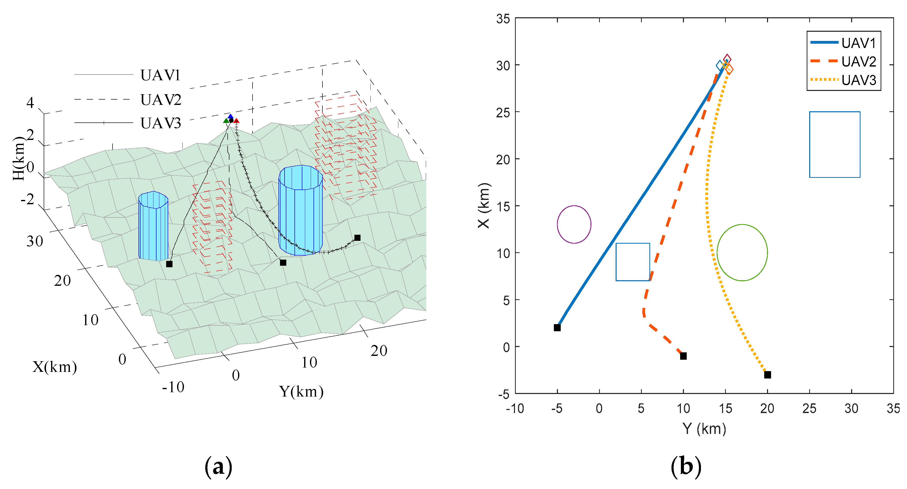
4.2. Path Planning for 3-D Formation Rendezvous

In the case of 3-D, obstacles are modeled as cylinders and no-fly zones are represented by rectangles with infinite heights. The initial poses of UAVs and the formation poses are given in Table 5. The desired formation configuration is the same as above. The maximum curvature and torsion of UAVs are κ max = τ max = 2 km 1 . The terrain is modeled using Equation (13). Other conditions and parameters are the same as above.
The paths of UAVs generated by the proposed DCPSO with cooperation in 3-D environments are shown in Figure 6. The curvature and torsion variations with respect to path length of each UAV are given in Figure 7. The length of three paths and their minimum separation distances are given in Table 6. Simulation results show that all three paths avoid the obstacles, no-fly zones, and the terrain. Both the curvature and torsion of the three paths change continuously while meeting the maximum-curvature and maximum-torsion constraints of UAVs. Meanwhile, the maximum difference of lengths is only 0.0081 km, which means simultaneous arrival of UAVs can be achieved and no collision happens between UAVs. Therefore, the algorithm proposed in this paper is also suitable in cooperative path-planning for UAV formation rendezvous in 3-D environments.

5. Conclusions

In this paper, a distributed cooperative particle swarm optimization (DCPSO) algorithm was proposed to generate a set of spatial paths for multi-UAVs that execute formation rendezvous missions. The quantic PH curve was used as the path because of its curvature continuity. In the DCPSO algorithm, the particles in each sub-swarm updated their positions and velocities separately, then they communicated with other sub-swarms to modify their fitness to realize simultaneous arrival under constraints. Some key points are illustrated as follows:
(1) Considering the kinematic constraints of UAV and collision avoidance, the proposed path planning method could generate simultaneous arrival paths for UAV formation rendezvous.
(2) Compared with the cooperative co-evolutionary algorithm (CCGA), the proposed algorithm could jump out of local optimum easily and had a better stability.

Author Contributions

Conceptualization, X.Z. and Z.Z.; methodology, Z.S.; software, Z.S.; formal analysis, Z.S.; writing—review and editing, Z.S. and F.Y.

Funding

This research was funded by Civil Aircraft Special Project (MJ-2015-F-009), National Key R&D Program in Shaanxi Province (2018ZDCXL-GY-03004).

Conflicts of Interest

The authors declare no conflict of interest.

References

  1. San Juan, V.; Santos, M.; Andujar, J.M. Intelligent UAV Map Generation and Discrete Path Planning for Search and Rescue Operations. Complexity 2018, 2018, 6879419. [Google Scholar] [CrossRef]
  2. Padro, J.C.; Munoz, F.J.; Planas, J.; Pons, X. Comparison of four UAV georeferencing methods for environmental monitoring purposes focusing on the combined use with airborne and satellite remote sensing platforms. Int. J. Appl. Earth Obs. Geoinf. 2019, 75, 130–140. [Google Scholar] [CrossRef]
  3. Zhen, Z.Y.; Xing, D.J.; Gao, C. Cooperative search-attack mission planning for multi-UAV based on intelligent self-organized algorithm. Aerosp. Sci. Technol. 2018, 76, 402–411. [Google Scholar] [CrossRef]
  4. Morganti, C.; Perdon, A.M.; Conte, G.; Scaradozzi, D. Multi-Agent System Theory for Modelling a Home Automation System. In International Work-Conference on Artificial Neural Networks; Springer: Berlin/Heidelberg, Germany, 2009; pp. 585–593. [Google Scholar]
  5. Friedrich, M.; Hofsaess, I.; Wekeck, S. Timetable-based transit assignment using branch and bound techniques. Transp. Res. Rec. 2001, 1752, 100–107. [Google Scholar] [CrossRef]
  6. Burlacu, A.; Kloetzer, M.; Mahulea, C. Numerical Evaluation of Sample Gathering Solutions for Mobile Robots. Appl. Sci. 2019, 9, 791. [Google Scholar] [CrossRef]
  7. Olfati-Saber, R. Flocking for multi-agent dynamic systems: Algorithms and theory. IEEE Trans. Autom. Control 2006, 51, 401–420. [Google Scholar] [CrossRef]
  8. Rezaee, H.; Abdollahi, F. Mobile robots cooperative control and obstacle avoidance using potential field. In Proceedings of the 2011 IEEE/ASME International Conference on Advanced Intelligent Mechatronics, Budapest, Hungary, 3 July 2011–7 July 2011; pp. 61–66. [Google Scholar]
  9. Rezaee, H.; Abdollahi, F. A decentralized cooperative control scheme with obstacle avoidance for a team of mobile robots. IEEE Trans. Ind. Electron. 2014, 61, 347–354. [Google Scholar] [CrossRef]
  10. Nguyen, T.; La, H.M.; Le, T.D.; Jafari, M. Formation control and obstacle avoidance of multiple rectangular agents with limited communication ranges. IEEE Trans. Control Netw. Syst. 2017, 4, 680–691. [Google Scholar] [CrossRef]
  11. Roberge, V.; Tarbouchi, M.; Labonte, G. Comparison of Parallel Genetic Algorithm and Particle Swarm Optimization for Real-Time UAV Path Planning. IEEE Trans. Ind. Inform. 2013, 9, 132–141. [Google Scholar] [CrossRef]
  12. Duguleana, M.; Mogan, G. Neural networks based reinforcement learning for mobile robots obstacle avoidance. Expert Syst. Appl. 2016, 62, 104–115. [Google Scholar] [CrossRef]
  13. LaValle, S.M. Planning Algorithms; Cambridge University Press: Cambridge, UK, 2006; pp. 1–826. [Google Scholar]
  14. Manathara, J.G.; Ghose, D. Rendezvous of multiple UAVs with collision avoidance using consensus. J. Aerosp. Eng. 2012, 25, 480–489. [Google Scholar] [CrossRef]
  15. Mclain, T.W.; Beard, R.W. Coordination Variables, Coordination Functions, and Cooperative Timing Missions. J. Guid. Control Dyn. 2005, 28, 150–161. [Google Scholar] [CrossRef]
  16. Choe, R.; Puignavarro, J.; Cichella, V.; Xargay, E.; Hovakimyan, N. Cooperative Trajectory Generation Using Pythagorean Hodograph Bézier Curves. J. Guid. Control Dyn. 2016, 39, 1–20. [Google Scholar] [CrossRef]
  17. Lin, Z.; Liu, H.T. Consensus based on learning game theory with a UAV rendezvous application. Chin. J. Aeronaut. 2015, 28, 191–199. [Google Scholar] [CrossRef] [Green Version]
  18. Yao, W.R.; Qi, N.M.; Liu, Y.F. Online Trajectory Generation with Rendezvous for UAVs Using Multistage Path Prediction. J. Aerosp. Eng. 2017, 30, 04016092. [Google Scholar] [CrossRef]
  19. Ismail, A.; Bagula, B.A.; Tuyishimire, E. Internet-Of-Things in Motion: A UAV Coalition Model for Remote Sensing in Smart Cities. Sensors 2018, 18, 2814. [Google Scholar] [CrossRef]
  20. Shanmugavel, M.; Tsourdos, A.; White, B.; Żbikowski, R. Co-operative path planning of multiple UAVs using Dubins paths with clothoid arcs. Control Eng. Pract. 2010, 18, 1084–1092. [Google Scholar] [CrossRef]
  21. Xing, Z.; Jie, C.; Xin, B.; Peng, Z. A memetic algorithm for path planning of curvature-constrained UAVs performing surveillance of multiple ground targets. Chin. J. Aeronaut. 2014, 27, 622–633. [Google Scholar] [Green Version]
  22. Tsourdos, A.; White, B.; Shanmugavel, M. Cooperative Path Planning of Unmanned Aerial Vehicles; John Wiley and Sons, Ltd.: Chichester, UK, 2010. [Google Scholar]
  23. Foo, J.L.; Knutzon, J.; Kalivarapu, V.; Oliver, J.; Winer, E. Path planning of unmanned aerial vehicles using B-splines and particle swarm optimization. J. Aerosp. Comput. Inf. Commun. 2009, 6, 271–290. [Google Scholar] [CrossRef]
  24. Alves Neto, A.; MacHaret, D.G.; Campos, M.F.M. On the generation of trajectories for multiple UAVS in environments with obstacles. J. Intell. Robot. Syst.Theory Appl. 2010, 57, 123–141. [Google Scholar] [CrossRef]
  25. Kang, S.; Choi, H.; Kim, Y. Formation flight and collision avoidance for multiple UAVs using concept of elastic weighting factor. Int. J. Aeronaut. Space Sci. 2013, 14, 75–84. [Google Scholar] [CrossRef]
  26. Farouki, R.T.; Sakkalis, I. Pythagorean hodographs. IBM J. Res. Dev. 1990, 34, 736–752. [Google Scholar] [CrossRef]
  27. Walton, D.J.; Meek, D.S. A pythagorean hodograph quintic spiral. Comput. Aided Des. 1996, 28, 943–950. [Google Scholar] [CrossRef]
  28. Walton, D.J.; Meek, D.S. Planar G 2 transition with a fair Pythagorean hodograph quintic curve. J. Comput. Appl. Math. 2002, 138, 109–126. [Google Scholar] [CrossRef]
  29. Farouki, R.T.; Al-Kandari, M.; Sakkalis, T. Hermite Interpolation by Rotation-Invariant Spatial Pythagorean-Hodograph Curves. Adv. Comput. Math. 2002, 17, 369–383. [Google Scholar] [CrossRef]
  30. Farouki, R.T.; Neff, C.A. Hermite interpolation by Pythagorean hodograph quintics. Math. Comput. 1995, 64, 1589–1609. [Google Scholar] [CrossRef]
  31. Farouki, R.T. Elastic bending energy of Pythagorean-hodograph curves. Comput. Aided Geom. Des. 1996, 13, 227–241. [Google Scholar] [CrossRef]
  32. Korayem, M.H.; Hoshiar, A.K.; Nazarahari, M. A hybrid co-evolutionary genetic algorithm for multiple nanoparticle assembly task path planning. Int. J. Adv. Manuf. Technol. 2016, 87, 3527–3543. [Google Scholar] [CrossRef]
  33. Qu, H.; Xing, K.; Alexander, T. An improved genetic algorithm with co-evolutionary strategy for global path planning of multiple mobile robots. Neurocomputing 2013, 120, 509–517. [Google Scholar] [CrossRef]
  34. Shorakaei, H.; Vahdani, M.; Imani, B.; Gholami, A. Optimal cooperative path planning of unmanned aerial vehicles by a parallel genetic algorithm. Robotica 2016, 34, 823–836. [Google Scholar] [CrossRef]
  35. Li, Y.H.; Zhan, Z.H.; Lin, S.J.; Zhang, J.; Luo, X.N. Competitive and cooperative particle swarm optimization with information sharing mechanism for global optimization problems. Inf. Sci. 2015, 293, 370–382. [Google Scholar] [CrossRef]
  36. Tian, D.; Shi, Z. MPSO: Modified particle swarm optimization and its applications. Swarm Evolut. Comput. 2018, 41, 49–68. [Google Scholar] [CrossRef]
  37. Suresh, K.; Kumarappan, N. Hybrid improved binary particle swarm optimization approach for generation maintenance scheduling problem. Swarm Evolut. Comput. 2013, 9, 69–89. [Google Scholar] [CrossRef]
  38. Tian, D.P. Particle Swarm Optimization with Chaos-based Initialization for Numerical Optimization. Intell. Autom. Soft Comput. 2018, 24, 331–342. [Google Scholar] [CrossRef]
  39. Fu, H.; Li, Z.; Liu, Z.; Wang, Z. Research on Big Data Digging of Hot Topics about Recycled Water Use on Micro-Blog Based on Particle Swarm Optimization. Sustainability 2018, 10, 15. [Google Scholar] [CrossRef]
  40. Liu, B.; Wang, L.; Jin, Y.H.; Tang, F.; Huang, D.X. Improved particle swarm optimization combined with chaos. Chaos Solitons Fractals 2005, 25, 1261–1271. [Google Scholar] [CrossRef]
Figure 1. Cooperative path-planning for unmanned aerial vehicle (UAV) formation rendezvous.
Applsci 09 02621 g001
Figure 2. Flow chart of distributed cooperative particle swarm optimization (DCPSO) with cooperation.
Applsci 09 02621 g002
Figure 3. Collision checking for two Pythagorean hodograph (PH) paths.
Applsci 09 02621 g003
Figure 4. Paths of UAVs for formation rendezvous. (a) Produced by DCPSO without cooperation; (b) produced by DCPSO with cooperation; (c) produced by CCGA.
Applsci 09 02621 g004
Figure 5. Curvature variations with respect to path length. (a) Produced by DCPSO without cooperation; (b) produced by DCPSO with cooperation; (c) produced by CCGA.
Applsci 09 02621 g005
Figure 6. Paths of UAVs for formation rendezvous in 3-D environments. (a) 3-D view; (b) top view.
Applsci 09 02621 g006
Figure 7. Curvature and torsion variations with respect to path length. (a) Curvature; (b) torsion.
Applsci 09 02621 g007
Table 1. Poses at UAVs’ starting points and rendezvous points (2-D).
UAVs/Rendezvous Point Pose   ( x , y , χ ) / ( km , km , rad )
UAV1 ( 2 , 5 , π / 6 )
UAV2 ( 1 , 10 , π / 4 )
UAV3 ( 3 , 20 , π / 5 )
Rendezvous point ( 35 , 15 , 0 )
Table 2. Desired formation configuration.
UAVs ( x f i , y f i ) / ( km , km )
UAV1(0.6, 0)
UAV2(–0.3, –0.6)
UAV3(–0.3, 0.6)
Table 3. Lengths of three paths and their minimum separation distances.
AlgorithmsL1 (km)L2 (km)L3 (km)dismin,12 (km)dismin,13 (km)dismin,23 (km)
DCPSO without cooperation35.061031.376034.34390.78631.08171.2000
DCPSO with cooperation35.061135.059035.06180.98681.08170.4879
Cooperative co-evolutionary genetic algorithms (CCGA)35.605435.520835.62080.95641.08170.3261
Table 4. Statistical results of 30 simulations.
Statistical ResultsDCPSO with CooperationCCGA
Amount of simulations3030
Number of success2713
Success rate0.90.433
Mean of L1 (km)35.061135.2982
Standard deviation of L1 (km)0.00010.1530
Mean of L2 (km)35.031035.1467
Standard deviation of L2 (km)0.06730.1413
Mean of L3 (km)35.059735.2329
Standard deviation of L3 (km)0.00540.1828
Average computation time(s)2.353.11
Table 5. Poses at UAV starting points and rendezvous point (3-D).
UAVs/Rendezvous Point Pose   ( x , y , z , χ , γ ) / ( km , km , km , rad , rad )
UAV1 ( 2 , 5 , 2.3 , π / 6 , π / 12 )
UAV2 ( 1 , 10 , 2 , π / 4 , π / 8 )
UAV3 ( 3 , 20 , 3.3 , π / 5 , π / 7 )
Rendezvous point ( 35 , 15 , 3 , π / 9 , 0 )
Table 6. Lengths of three paths and their minimum separation distances (3-D).
L1 (km)L2 (km)L3 (km)dismin,12 (km)dismin,13 (km)dismin,23 (km)
35.047035.043235.05130.95271.08171.2000

