3.1. Time-Invariant SISO TF Models
In
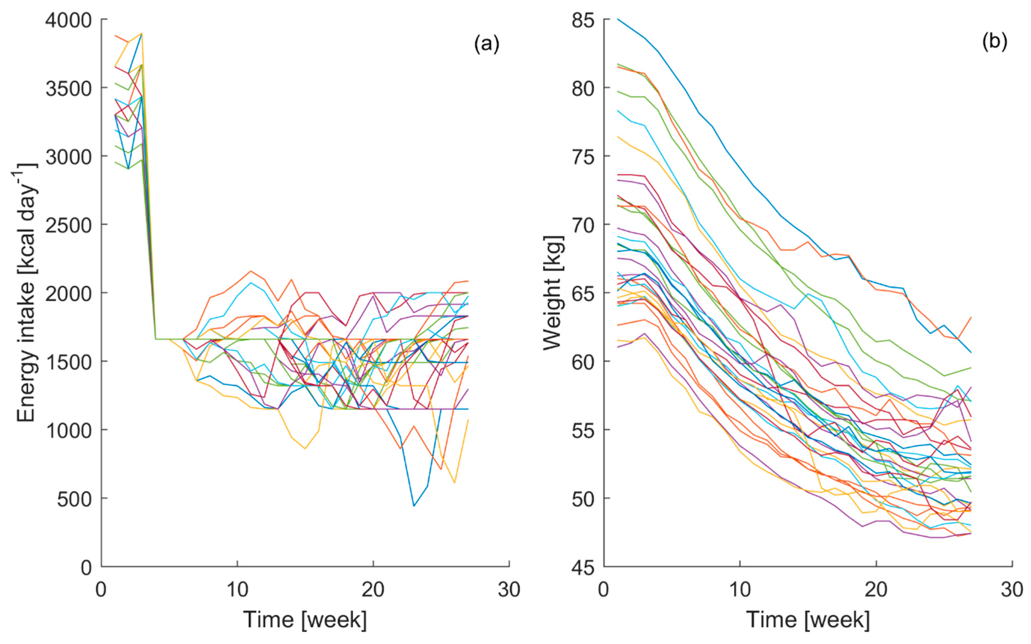
Figure 1, the gathered energy intake and bodyweight curves from the 32 participants are displayed.
The obtained data have shown clear interpersonal differences between participants in their energy intake and bodyweight curves during the course of the experiment. Even though during the control phase it is attempted to reduce the variability in the bodyweight among the participants, it can be seen that the individual variability in energy intake during the starvation stage of the experiment induced different responses in the bodyweight time course. Similar energy intake patterns lead to different bodyweight time courses, which highlights the individual characteristics of the biological process, emphasizing the importance of the aim of this study.
Therefore, using the Minnesota starvation experiment dataset, 32 sub-datasets are created using the bodyweight and energy intake from each individual participant. Using each sub-dataset, a system identification procedure is performed to define the best time-invariant parameters model structure needed to relate energy intake and bodyweight. In
Table 1, a summary is shown of the first and second order model performances in terms of
YIC and the goodness of fit,
.
Table 2 shows the Pearson correlation coefficients (
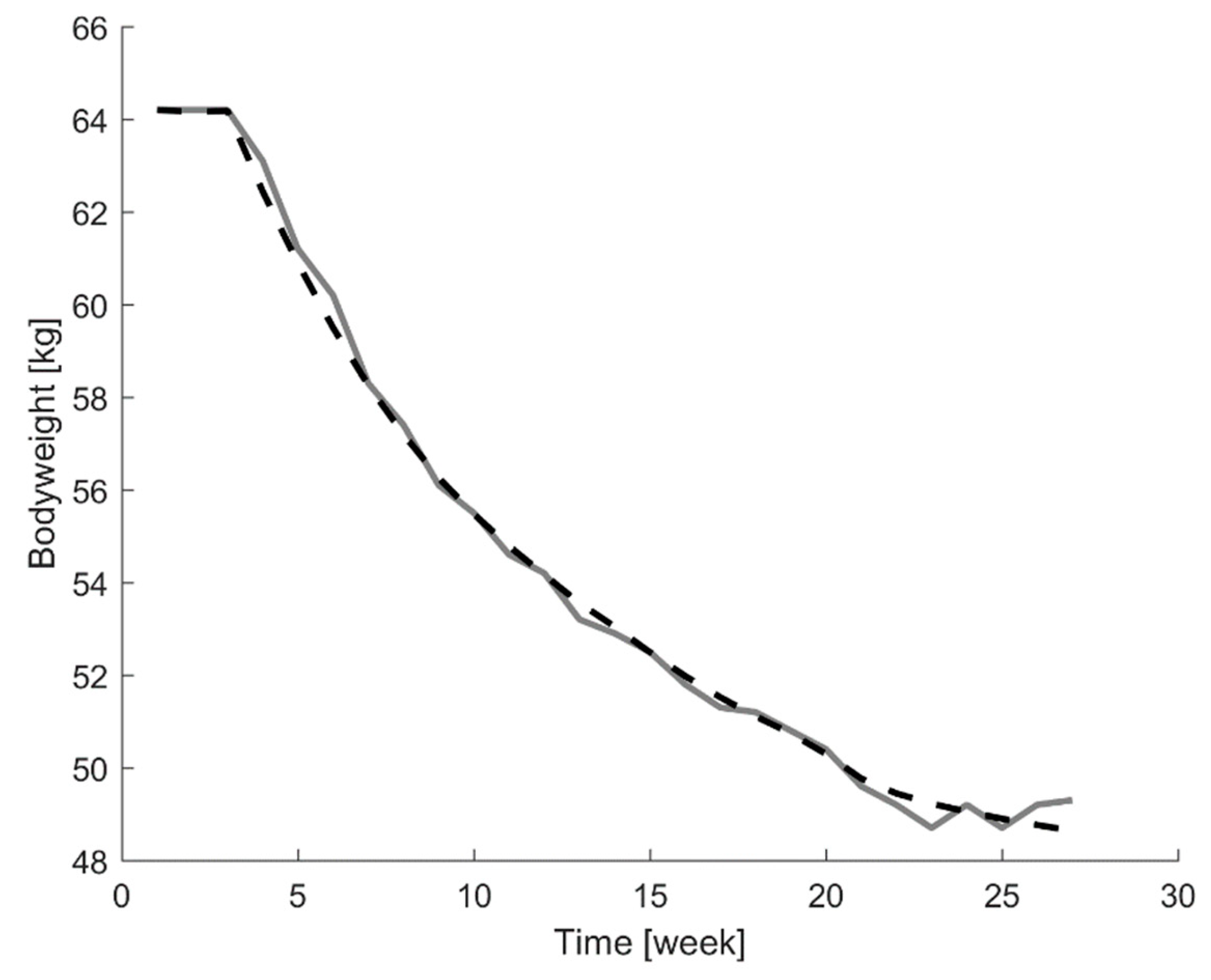
r), to assess the similarity between the model outputs and the weight curves from the participants. A representative example of the agreement between the measured and estimated bodyweight curves for one individual test participant (participant 8) in the Minnesota starvation experiment is displayed in
Figure 2.
The results have shown that a first order model is sufficient to characterize the impact of energy intake in bodyweight, as reflected by the superior
YIC,
, and a high Pearson correlation coefficient results (see
Table 1 and
Table 2). During the system identification process, the presence of delay was allowed, but the best results were always obtained when no delay (i.e.,
δ = 0) was present in the models. From a biological viewpoint this make sense, as metabolizing the ingested energy takes about 12 h, while the used time interval is one week (i.e., 168 h). Thus, the time delay between energy intake and bodyweight change reduces to nearly zero in terms of the used measurement interval of one week.
In addition, the YIC value also indicates that the parameters estimation when using a first order model is reliable. Ideally, it would be possible to define a first order model, using the average values of the different estimations of
a- and
b-parameters obtained for each subject, which would allow estimating the impact of bodyweight of a given energy intake. When the
a- and
b-parameters from the individual estimations are averaged together, the following model is obtained,
where
BW is bodyweight in kg,
EI is the energy intake in kcal day
−1 and
t is the time sample in weeks. It can be seen that the
b-parameter exhibits more variability than the
a-parameter. This is expected, taking into account the biological process under study. Translating the model to the biological process, it states that the bodyweight at time
t is the bodyweight of the time sample before plus a contribution of a certain percentage of the energy intake at time sample
t. Therefore, on one hand it is expected that the
a-parameter should be close to one and should not show too much variability between participants. On the other hand, the
b-parameter should resemble energy efficiency and thus it is expected to vary between the different individuals. From Equation (20), it can be the seen that the results matched perfectly this hypothesis. Running this average model in all datasets results in an average coefficient of determination of
= 0.3 ± 0.2. Therefore, by defining an average model in which an average
b-parameter value is set, the performance of the model drops drastically. In several previous studies [
24,
25,
26,
27,
28,
31,
32,
33], models were developed to estimate bodyweight changes in response to changes in the energy balance, taking into account energy intake and physical activity. These models are mechanistic models, using population-based average estimations of parameters to describe the energy balance equations. This explains the high standard deviation exhibited in the results of these models. The same is observed in this work, when an average time-invariant parameters model is developed. This clearly indicates the need for accurately estimating the proper
b-parameter value for each individual.
Therefore, from the system identification step it can be concluded that a first order transfer function model is sufficient to characterize the impact of energy intake on the bodyweight time course. However, it is necessary to use b-parameters that resemble the energy efficiency of the individual, and thus developing an average model is not a suitable approach. Moreover, it is expected that this energy efficiency would not only be individually different, but also change throughout the experimental period. Internal and external factors are expected to affect how a person translates the energy intake into a bodyweight change throughout the weight intervention process. Therefore, by including time-variant parameters in the model, it is expected to cope with these dynamic characteristic of the process. Thus, in the next section the results of the time-variant parameters modelling approach are described.
3.2. Time-Variant Parameters Models
By allowing the parameters to vary in time, it is expected to capture the changes induced in the energy efficiency by factors not taken explicitly into account in the model and, hence, obtain a more accurate estimation of bodyweight.
Firstly, the modelling accuracy is evaluated when modelling the complete experiment. In the previous section, it was shown that a first order transfer function model is sufficient to describe the relation between the energy intake and the bodyweight. Thus, a first order DARX model and a DLR model are tested. In
Table 3, the results from the modelling performance for the complete experiment, in terms of the
NRMSE and
r, are shown for both time-varying modelling approaches.
These results indicate that the DLR model provides a better and more consistent fitting agreement than the DARX model. Thus, from these results it seems that the DLR model outperforms the DARX approach. One of the reasons, which can explain this finding, could be the higher stochasticity behavior in the DLR model. Stochastic models can account for the variability among individuals in populations. Thus, a combination of deterministic and stochastic parts in the model allows quantifying both, the trend and the variability present in the process [
51]. Besides, in the work of [
2], weight loss is modelled by energy deficit, using energy flux balances. They found that when a stochastic component is added to the model the results improved. This is in line with the results obtained in this analysis. Allowing the time –variant model parameters to have a stochastic behavior, in order to characterize their time-evolution, improves the modelling performance. However, this analysis just confirms that a first order model with time-variant parameters allows characterizing the relation between energy intake and bodyweight time-course more accurately than using time-invariant parameters models, as expected. In order to develop a control system in the next phase, the model should not only describe the process accurately but also should exhibit suitable forecasting properties. Therefore, the forecasting capabilities of both time-variant parameters models are tested. In
Table 4 and
Table 5, the forecasting performance for the DLR and DARX models is displayed in terms of
MRPE.
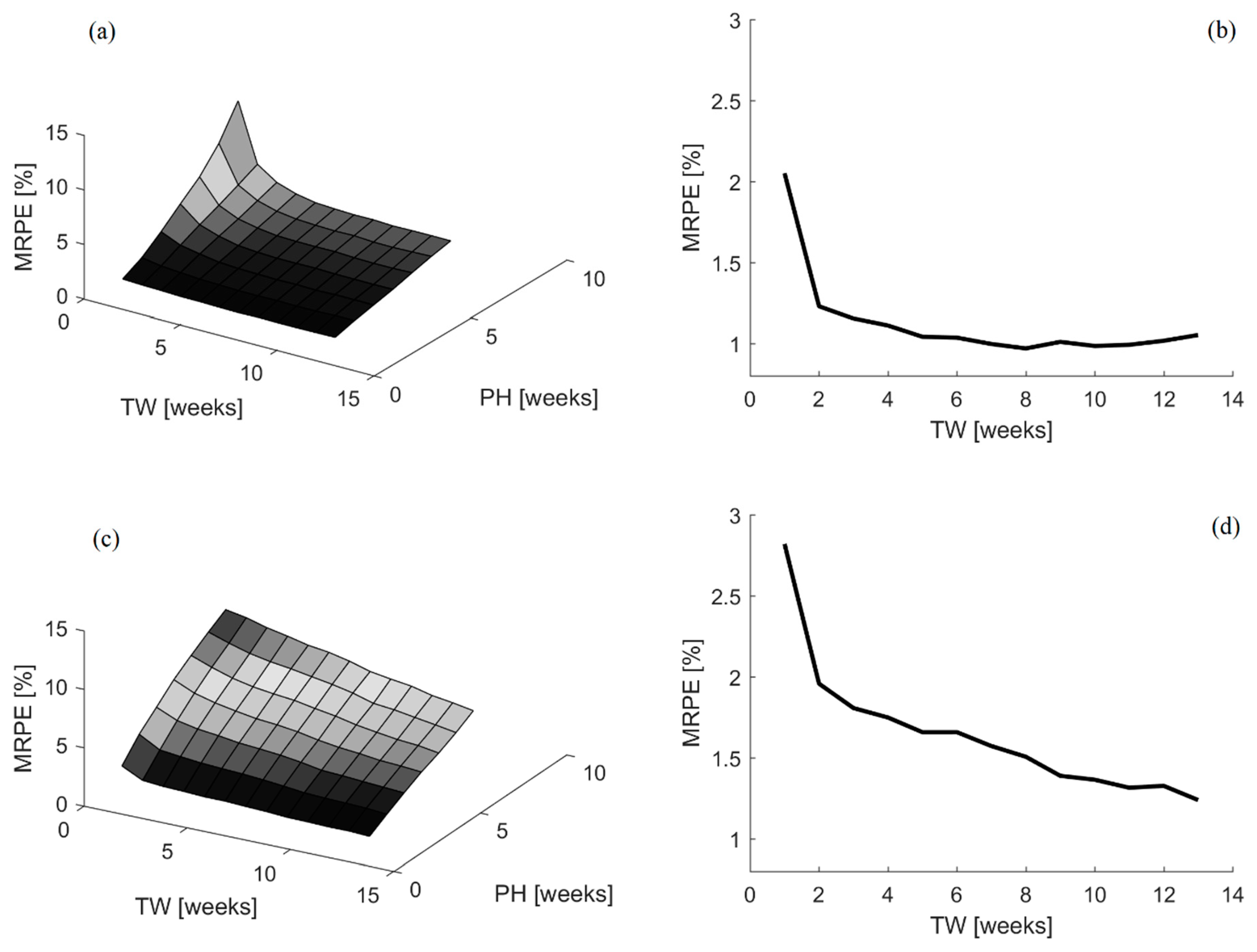
Besides, in
Figure 3, the results obtained for the different combinations of time window and prediction horizon sizes tested for both time-variant parameters models are displayed, together with a representative example for the one-week ahead prediction horizon forecasting results.
It is clear from the aforementioned results that the DARX model is able to achieve the best forecasting performance. Time window sizes ranging between 7 and 12 weeks lead to a MRPE of 1.01 ± 0.02%, on average, when using the DARX model. In the same range, the average MRPE for the DLR model is 1.53 ± 0.12%. Thus, there is a difference of 0.52% in favor of the DARX model prediction capabilities. Besides, the evolution of the MRPE among the different time window and prediction horizon sizes in the DLR model improves, as more data is included in the time window. Biologically, it is expected that the energy efficiency will vary with time and the current efficiency should be more relevant than the efficiency in past instances. Thus, it seems that the DLR model is not capturing fully the expected biological behavior of the process.
In contrast, the DARX model shows that increasing the window size improves the forecasting performance, but only until a certain range. Once this range is exceeded, the forecasting properties worsen again. This is expected, as the sliding time window with a fixed size should help in removing the impact of obsolete data in the model [
47]. Thus, this is more in line with what it is expected in terms of the biological process under study. Furthermore, it can be seen that the optimal time window size changes according to the prediction horizon size. For instance, if the prediction horizon is raised to 4–5 weeks, thus over a month time, the MRPE error ranges between 2.5–3% and the optimal time window size range increases to 10–14 weeks.
The prediction of bodyweight using a recursive linear regression approach based on time-variant parameters has been already tested on broiler chickens [
47]. In that study, the lowest
MRPE reaches a value of 1.4% for a prediction horizon of 1 day and the highest
MRPE is 4.1% for a prediction horizon of 7 days, when broiler chickens are fed ad libitum [
47]. These results illustrate that using time-variant parameters models to predict human bodyweight is highly accurate, improving the previous results.
Lastly, it is important to mention that because little information on energy expenditure is known, the bodyweight predictions are based solely on energy intake. The data from the Minnesota starvation experiment include merely estimations of the resting energy expenditure on the week prior to the starvation phase and at the end of the starvation phase. Thus, calculating the weekly energy balance is not possible. There are several models in literature that attempt to address this characteristic during a weight program intervention by using complex mechanistic models based on systems of one dimensional differential equations [
28,
29,
31,
32]. Although these theoretical models resemble accurately the dynamic process of bodyweight change, the large amount of model parameters are estimated based on averages from population studies [
32] and do not take into account the changes in the values of the model parameters throughout the experimental period [
11]. In the modelling framework proposed in this study, not only the dynamic evolution through time, but also the dynamics induced by the impact of internal and external factors in the model parameters are taken into account implicitly by the model. This allows designing more compact models, reducing greatly their complexity while capturing the most relevant dynamics of the process. In future, if both energy intake and expenditure would be available, a time-variant model in which both are used as inputs could be developed. Moreover, gathering regular information about the time course of fat body mass and lean body mass would allow developing a time-variant model, whose model parameters could be related to existing mechanistic equations describing bodyweight component changes in response to changes in energy intake and energy expenditure. On one hand, this would help dietitians to develop further the current mechanistic expressions to describe more accurately the bodyweight change process. On the other hand, it would enable them to evaluate and adapt in real-time the impact of the suggested dietary energy intake to achieve a desire bodyweight change at individualized patient level.
In summary, these results show that a time-variant parameters model allows characterizing accurately the dynamics of a body weight change induced by a change in dietary energy intake. Using a window size of seven weeks of dietary energy intake allows forecasting bodyweight one-week ahead with a MRPE of 1.04% and four-weeks ahead with a MRPE of 2.53%. Therefore, from this analysis with time-variant models, it seems that a first order DARX model is the best model choice when balancing fitting agreement and forecasting performance. Besides, it seems to describe more accurately the biological process under study. Therefore, this model is considered the best option to develop a model-predictive control to estimate the energy intake needed to achieve a desired bodyweight change. In the next section, the model predictive controller is developed and tested. When using the time-variant parameters model in the controller, the time window size of seven weeks is selected. It should be noted that even though in this study the time window size is fixed, it would be possible to perform a similar analysis as the one described in this section to estimate in real-time which would be the optimal time window size to be used in the controller’s model for each individual.
3.3. Simulation Model Predictive Control
Several MPC systems are developed using both the time-invariant and time-variant parameters transfer function models tested in the previous sub-sections. In order to test the capabilities of the controller for each individual participant, the bodyweight collected during the experiment is used as reference bodyweight curve and then the energy intake advised by the controller is compared with the measured energy intake. First, simulations are performed without any constraint to the system. Next, simulations with constraints are performed as well. In
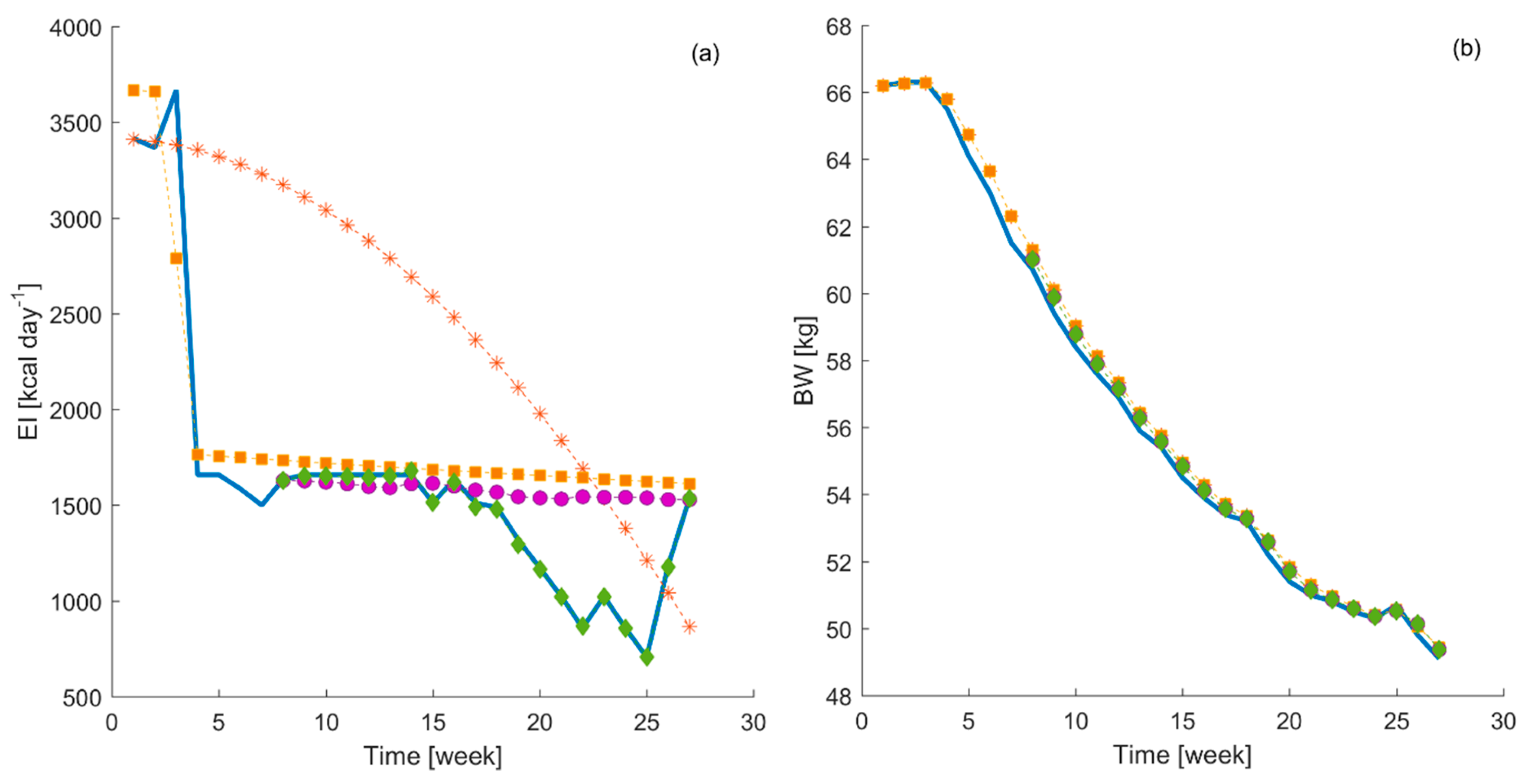
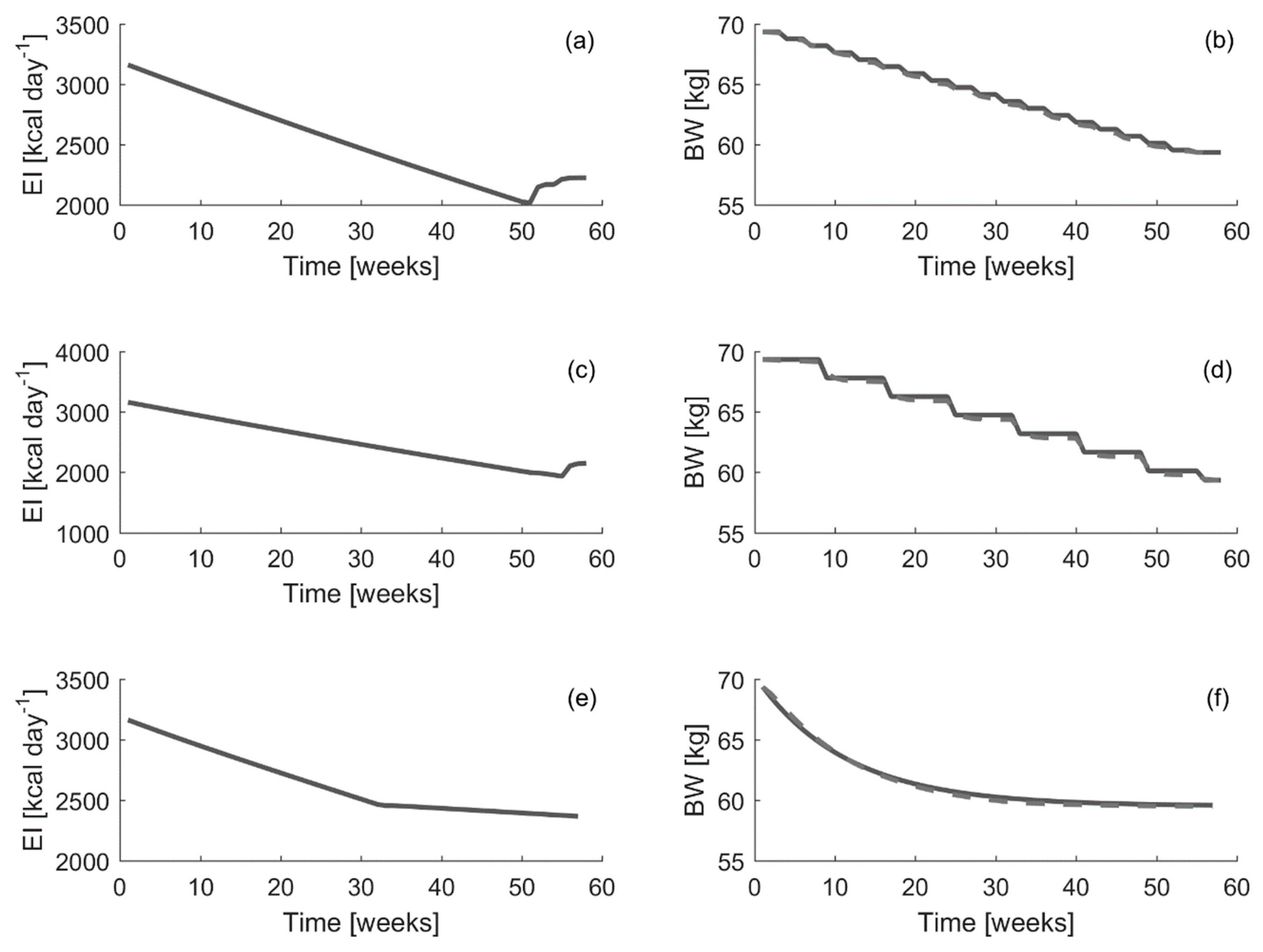
Figure 4, a comparison between the energy intake suggested by the different controllers and the energy intake collected during the experiments is displayed.
The results have shown that the developed MPC, using the time-variant parameters DARX model, suggested an energy intake which is closest (see
Table 6) to the actual energy intake collected during the experiment in comparison to that suggested by the MPC developed using time-invariant models. The MPC developed using the time-invariant model with constraints and the one using the DARX model without constraints perform similarly. Finally, the MPC developed using the time-invariant model and without constraints suggests an energy intake, which follows completely different dynamics. In addition, all MPC systems tested generate similar bodyweight curves, which follow closely the reference bodyweight curve. In order to quantify this visual inspection,
Table 6 shows a summary of the
NRMSE,
RMSE and
r values when comparing the measured energy intake and bodyweight curves with those estimated from the different controller simulations. Besides, the
RMSE between the final weight achieved by the participant and the final weight obtained in the different controller simulations is summarized in
Table 7.
It can be seen that the best performance is obtained when using the DARX model in the controller with constraints in the simulation. The RMSE for bodyweight and energy intake is only 260 g and 9 kcal day−1, respectively. Moreover, the difference between the final bodyweight and energy intake values from all MPC’s and the measured ones during the experiment are, on average, lower than 440 g and 12 kcal day−1, respectively.
These results highlight again the need to use individualized time-variant parameters models to develop a MPC capable to manage automatically the individualized advice of energy intake to achieve a desire bodyweight change. However, this does not necessarily mean that the other MPCs are suggesting completely wrong energy intake levels. As it can be seen in
Figure 4, all outcome bodyweight curves from the MPCs follows closely the reference one. Thus, these suggested energy intake curves should be understood as alternative possibilities that, in principle, would have taken the participant to similar end bodyweight without lowering suddenly the energy intake, but by lowering the energy intake following another pattern. When starting to lower the energy intake following one of these alternative curves, it would be still needed to develop a time-variant model to monitor the performance of the test subject in real-time and adapt the suggested curves to the new conditions. In this regard, these capabilities can be exploited by dietitians to determine which is the healthier alternative for an individual patient to achieve the desire bodyweight change according to its response to the initial treatment through time.
Thus, in order to test the MPC system capabilities to follow theoretical reference curves, three different theoretical bodyweight curves are defined according to the procedure described in
Section 2.3 of the Material and Methods section. In
Figure 5, the different energy intake curves suggested by the controller are displayed. In addition, the resulting estimated weight curves obtained when following these suggestions, compared with the defined theoretical ones, are displayed as well. In order to perform these simulations, the average time-invariant model obtained in
Section 3.1 of this section is used as model for the controller. This approach cannot be tested with the time-variant parameters DARX models, as there is no actual data collection from the participants following these theoretical curves.
It can be seen that the energy intake curves suggested by the controller are similar. The main difference is the energy intake change rate over consecutive weeks. Depending on the theoretical bodyweight curve used as reference, the energy intake suggested for an average individual decreases faster or slower in consecutive weeks. The
NRMSE,
RMSE and
r describing the differences between the reference bodyweight curve and the bodyweight curves achieved with the control simulation are summarized in
Table 8.
Table 9 shows the
RMSE between the final bodyweight value from the controllers and the one from the theoretical reference curve.
It can be seen that the RMSE errors, when comparing the complete curves or just the final values, are small, less than 200 g on average, in all cases. Thus, the MPC controller is able to follow closely a predefined theoretical bodyweight curve. Therefore, the MPC developed in this study may be used to set a theoretical bodyweight reference curve and evaluate the energy intake curve suggested to follow the given bodyweight curve in order to achieve the desired final weight.
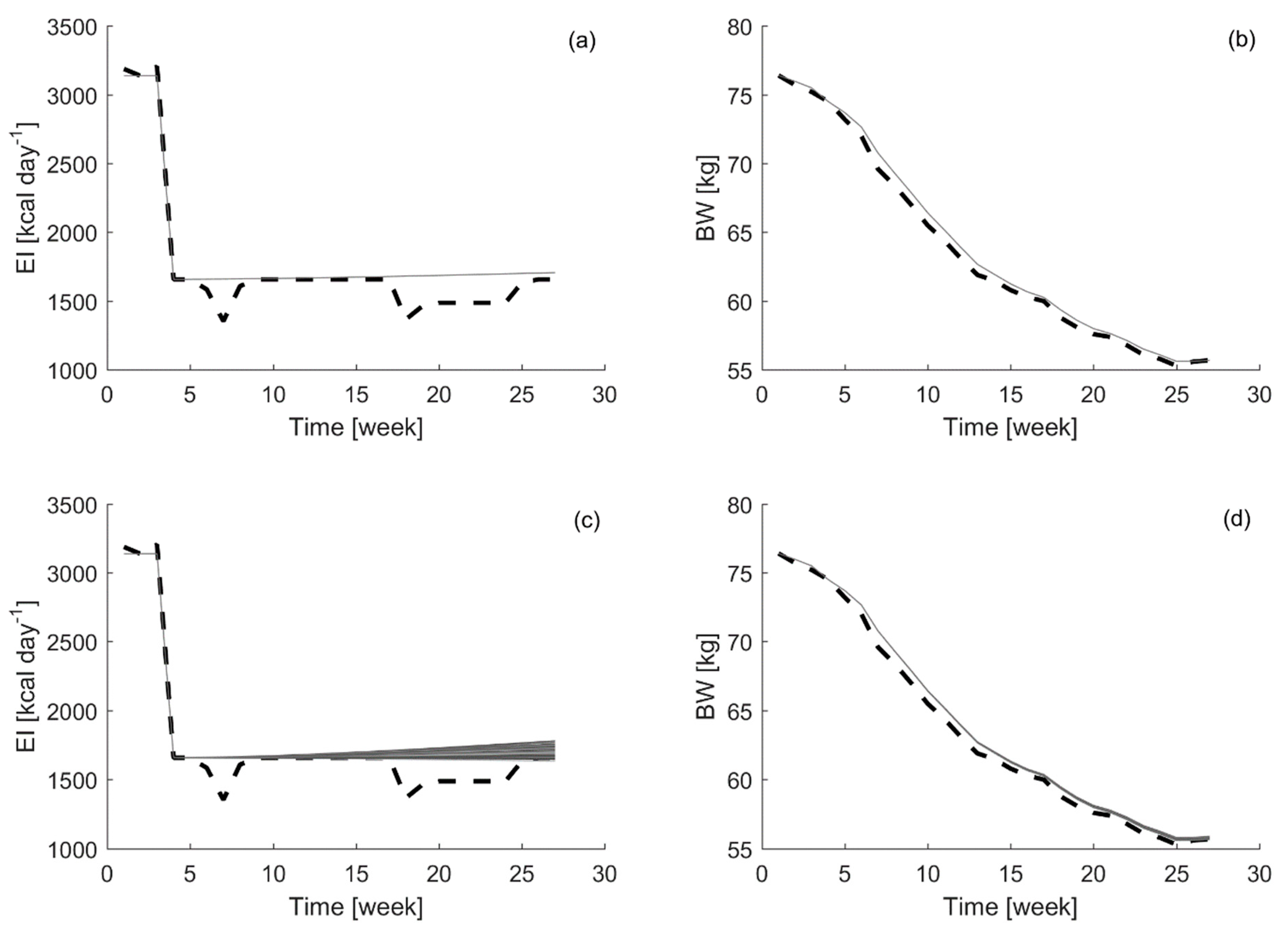
Finally, as the last part of the analysis, the robustness of the controller is tested. A random contribution, at the level of the standard error in the parameters estimations (10%), is added as uncertainty to the
a- and
b-parameters of the time-invariant model. Using Monte Carlo simulations, the robustness of the model is tested, generating 100 realizations varying
a- or
b-parameter estimations. In
Figure 6, examples of the suggested energy intake and bodyweight curves obtained from these 100 Monte Carlo simulations, adding uncertainty in the
a- and
b-parameters, respectively, are shown.
The results have shown how the controller’s suggestions for energy intake are much less sensitive to the uncertainty in the a-parameter than in the b-parameter. This is expected as the b-parameter represents the energy intake efficiency; thus, slight changes in this parameter induce changes in the energy required to achieve a target bodyweight. However, uncertainty in the a-parameter should be limited as well, because an increase in uncertainty may lead to an unstable model. Therefore, these results point out again towards the need to use time-variant parameters models, such the DARX model tested in this study, to obtain accurate estimations of the model parameters and their time evolution for individual participants. Accounting in the model parameters for this variability improves considerably the capabilities of the MPC to suggest energy intake levels which take the individuals variability into account, enabling it to get the closest possible to the targeted bodyweight.
In [
41], the growth trajectory of broiler chickens is controlled based on an adaptive dynamic model. Here, the performance of the MPC algorithm is quantified by calculating the mean relative error (MRE) between the actual and target weight trajectory of the broiler chickens. The MRE values ranged between 3.7% and 7.0%. For broiler chickens, it is important that the actual growth trajectory resembles the target trajectory, in order to suppress negative effects associated with fast growing broiler chickens. Examples of negative effects include decreased reproduction capacity of the breeder stock, increased body fat deposition and metabolic diseases, such as sudden death syndrome [
41]. In [
43], the MPC developed in [
41] was tested in commercial broiler settings. In this case, the MRE ranged between 6% and 11% under these conditions. Translating the NRMSE and RMSE results from this work to MRE values, obtains, on average, a MRE of 0.65 ± 0.07% and 0.34 ± 0.06% when comparing the experimental measured bodyweight curve for each participant and the bodyweight curve obtained following the suggestions from the MPC using time-invariant parameters and time-variant parameters models, respectively. Moreover, MRE of 0.12 ± 0.01%, 0.18 ± 0.02% and 0.15 ± 0.03% are obtained when comparing the theoretical bodyweight reference trajectory curves and those obtained when following the MPC suggestions for the theoretical reference trajectories 1, 2 and 3, respectively. Therefore, the MPC’s developed in this work show that they are capable of following different bodyweight reference trajectories accurately. Similarly as in the case of the time-variant parameters models, the MPC’s developed in this work exhibit a high accuracy when compared with the ones developed for livestock applications. Thus, this enables dietitians to develop a theoretical bodyweight curve and test the energy intake suggested to fulfill this goal in an individualized manner for their patients. Besides, taking advantage of the adaptive capabilities of the MPC, it is possible to modify in real-time this bodyweight reference trajectory according to the performance of the patient and health considerations.
In [
11,
34], dynamic models are developed to control bodyweight dynamics. These models are dynamic in the sense of accounting for the time evolution of the bodyweight and energy processes. However, these models do not account for the time evolution of the model parameters or the individualized estimation of those parameters working in real-time. These dynamic models still rely on average mechanistic descriptions of the bodyweight and energy flux dynamics. Thus, these approaches lack the adaptability characteristics of the MPC developed in this work. However, a MPC as developed in this work has still some drawbacks to be taken into account in the future. No information on the ratio of carbohydrates, lipids and proteins with respect to the total energy intake is provided. In addition to the total energy intake, further optimization of the MPC algorithm can include suggestions on the ratio of carbohydrates, lipids and proteins based on the recommended dietary allowances. An important factor influencing the dietary behavior is the degree of saturation. Food with a high energy density usually ensures a low degree of satiety. Therefore, food with a low energy density is usually recommended, as it provides a longer period of satiety [
52]. In [
12], it is shown that combining current methods to deal with bodyweight changes with mHealth applications may enhance the performance of the first ones. Therefore, on the one hand, the current applications may benefit from including such a MPC as developed in this work. By providing more individual accurate estimations of energy intake and bodyweight change levels, it is expected to enhance the engagement to the mHealth technology and the adhesion to its suggestions, improving weight management [
33]. On the other hand, if further development of apps and wearables enhance the characterization of the energy intake, physical activity and other related physiological variables, the MPC developed in this work can be extended to manage more accurately the metabolization and energy flux balances processes. In such a situation, a comparison with the existing mechanistic models would allow extracting more biological and physical information while keeping the real-time and automatic properties of the controller.
To sum up, it can be seen that such a MPC system may help people to manage and control their bodyweight in real time. Taking advantage of the new possibilities offered by wearables and smartphones, an individual can gather real-time information about their energy intake, bodyweight and activity. Then, mHealth applications may exploit such compact and accurate MPC algorithms to manage body weight change taking advantage of the data gathered. This enables a target bodyweight or bodyweight reference curve to be defined and suggestions for the energy intake needed to achieve this goal to be made. Besides, the MPC system may be a useful tool for dietitians as well. They can develop theoretical bodyweight curves for losing weight using biological and medical information and simulate the energy intake suggested to follow this curve at individual patient level as close as possible. Moreover, at certain points in the treatment, this theoretical curve can be adapted according to the performance of the patient and medical considerations. Thus, the MPC system can be used not only to simulate an energy intake pattern according to a predefined bodyweight curve, but also to monitor the impact of the strategy in individual patients and adapt the strategy accordingly throughout the bodyweight change process.
3.4. Current Limitations and Future Perspectives
The Minnesota starvation experiment was performed in 1944 to investigate the psychological and physiological effects of severe dietary restriction [
53]. The experiment was designed to mimic the dietary conditions of prisoners during World War II. Therefore, due to both the period in which the experiment was performed and the focus, only male participants were selected. This restriction in energy intake is not a recommended method to lose weight, as the energy intake is lower than the minimum requirements. However, this abrupt change in energy intake presents the perfect conditions to perform an analysis of the system’s dynamics and the modelling of body weight in response to energy intake. Unfortunately, the experiment has some limitations with respect to age, gender, size of the study population, and BMI category. The population of the Minnesota starvation experiment counted 32 male participants. The size of the population was small and the population did not represent differences in gender, BMI category and age. A study, performed on male and female mice, showed that the metabolic processes during bodyweight dynamics are gender-dependent [
54]. Therefore, it is necessary to verify and model the body weight dynamics of both males and females. The age of the participants varied between a limited range of 20 and 33 years. Metabolic processes are not only dependent on the gender but also on the age. To estimate the basal metabolic rate (BMR), the equations in [
49] are often used and are different depending on gender and age. Calculation of BMR is based on height and weight. In the Minnesota starvation experiment, the average body weight and BMI of the participants prior to the starvation phase were 69.36 kg and 21.7, respectively. All participants apart from one had a BMI in the normal category. Only one subject was slightly overweight with a BMI of 25.4. The aim of this study is to make a first step towards designing a controller to help overweight or obese people lose body weight. However, the constructed controller is based on data of 32 male participants within the normal BMI category. Regardless of the limited subject variation, the controller should eventually depend on time-variant parameters opposed to time-invariant parameters. The benefit of using time-variant parameters is that if the underlying metabolic processes are changed due to unknown factors, the parameters are updated in order to predict future body weight more accurately.
The modelling framework also has certain limitations. It is known that the weight loss intervention strategies will be affected by external factors [
55], such as psychological [
56,
57,
58,
59], occupational [
60,
61,
62,
63], and metabolic factors [
64,
65], besides their combined effects [
66,
67]. These external factors will affect the weight loss intervention, as well as its maintenance in the long term [
68,
69]. Besides, there is a high degree of heterogeneity in the impact of these factors both, during and after a weight intervention [
70]. In principle, the modelling framework developed in this study cannot provide directly any information about this matter during its application throughout the weight intervention. However, there is an aspect in the proposed modelling approach, which can actually allow getting some insight in this regard. One of the reasons for allowing the parameters to vary with time is to capture the contribution of external factors, which impact the process under study but which are not taken explicitly into account in the model. Therefore, the time evolution of the model parameters can be understood as a summary of the contribution of each individual external factor, besides the inherent time evolution related to the process input (energy intake in this study). This is the reason why, although we use a simple compact model based solely on energy intake and bodyweight, this allows describing accurately the weight loss intervention.
This, at first sight, model limitation actually provides one of the most interesting aspects for future improvement and development of the modelling approach. More specifically, it opens the possibility to use the time evolution of the model parameters as data-based reference to describe the impact of these external factors. If experiments, in which in a controlled manner a weight intervention is taking place and only one or a limited number of its external factors are allowed to vary, then the output from the current mechanistic expression can be tested against the time-variant model parameters. This would allow not only quantifying the impact of one or several of these external factors, but also gaining insight in how to refine the proposed mechanistic relations assumed for them. Yet, the validity of the proposed model could be validated too. Finally, the development of novel features in smartphone and wearable technologies continues growing exponentially. Therefore, it is expected that soon it will become possible to have available real-time measurements of more variables playing a role in the weight intervention. Thus, the model and controller proposed in this study could be expanded and refined in order to describe more accurately and gain more insight in the weight intervention.

 ,
, 


