Abstract
Since pipelines experience the largest deformation during lowering-in, structural analysis for this construction sequence should be performed to ensure structural safety. In this study, a new analytical model named the “segmental pipeline model” was developed to predict the structural behavior of the pipeline. This analytical model consists of several segmental elements to represent various boundary and contact conditions. Therefore, the segmental pipeline model can consider the geometric configuration and characteristics of pipelines that appear during lowering-in. Adopting the Euler-Bernoulli beam and two-parameter beam on elastic foundation theory, the new model takes the effect of the soil and axial forces acting on the pipelines into account. This paper compares the displacements, sectional bending moments and shear forces of the pipeline obtained from the analytical model and finite element (FE) analysis, where good agreement was demonstrated. Also, the paper presents three examples to demonstrate the applicability of the analytical model.
1. Introduction
A pipeline experiences large deformation and high stress during the construction process, especially during lowering-in. API STANDARD 1104–Appendix A limits the maximum stress during the construction sequence to 75% of the yield stress and defines it as the Specified Minimum Yield Strength (SMYS). In addition, this standard encourages a pipeline stress level check accompanied by construction procedure analysis, defined as an Engineering Critical Assessment (ECA) [1]. The finite element (FE) model, which has a strictly implemented boundary condition, can provide accurate analysis results but it requires large model preparation and computational times. On the other hand, the analytical model can offer a considerably shortened analysis time while providing appropriate response results, even though the analytical model has somewhat less accuracy than the FE model.
An elastic beam model partitioned or segmented according to the geometric deformation and loading condition was proposed by Scott et al. [2] and Duan et al. [3]. However, the proposed model has a limitation since the factors adopted for the analysis are determined by experience. Furthermore, the demand for continuity of the rotational angle at the boundary between each beam element is not satisfied since the boundaries are simplified into free or fixed ends. The proposed models are inconvenient as the factors adopted for the analysis were determined by construction conditions based on experience. Therefore, these models are unable to simulate various states of lowering-in.
Most analytical models for the structural behavior of buried pipelines mainly deal with the soil-pipeline interaction and stresses on pipeline. The simplest analytical modeling of a buried pipeline was proposed by Newmark and Rosenblueth [4] and Hall and Newmark [5]. In this model, the pipeline is assumed to be dominated by the deformation of the ground, so soil pipeline interactions cannot be considered. Wang et al. [6] and Nelson and Weidlinger [7] have proposed an analytical model for a quasi-static analysis considering the soil-pipeline interaction. This model is based on a spring supported beam to simulate buried pipelines. Although the analytical model can be estimated the axial deformation but the cross-section response of a pipeline may not be expressed in the model. To overcome this drawback, a shell models for pipelines have been developed [8,9,10]. Subsequently, Wong et al. [11], Datta et al. [12] and Takada and Tanabe [13] have proposed the soil-pipeline interaction using a plane strain model for the 3-D analysis of a pipeline. The cross sectional buckling and radial displacement can be evaluated using these models. However, in this shell modeling approach, it is difficult to consider the complete soil-pipeline interaction. Also the analysis procedures involve a series of equations, which in turn require intensive computational effort [14].
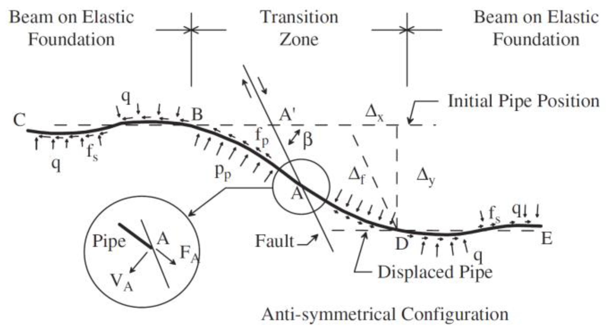
Another analytical model for the structural performance assessment of a pipeline buried in a fault zone was proposed by Kennedy et al. [15]. This model is assembled with both the beam on an elastic foundation (BOEF) and a cable element. However, this model does not correctly assume the maximum bending stress in an actual fault zone. Wang and Yeh [16], Karamitros et al. [17] and Trifonov and Cherniy [18] tried to overcome this shortcoming by modeling the pipeline partitioned with BOEF and a Euler-Bernoulli beam, as shown in Figure 1. In these models, the axial force of the pipeline due to fault displacement is appropriately considered but the axial forces are absent in the BOEF zone. Also, in the fault zone, the pipeline is modeled with the specified deformation and partitioning points. Due to its features, it is difficult to apply these models for the analysis of the lowering-in phase.

Figure 1.
Analytical model for the pipeline proposed by Wang [16] (as cited from Karamitros et al. [17]).
Dixon and Rutledge [19] developed natural catenary theory, forming the stiffened catenary theory to solve the pipeline laying problem. Catenary method is ordinary techniques to analyze pipelines and is used in pipeline modeling for offshore installations. However, this methodology is insufficient for analyzing the structural behavior of the dominant pipeline to the bending in the lowering phase. In the model developed by Lenci and Callegari [20], a combination of a rigid seabed or BOEF for the seabed and ‘cable or cable and elastic beam’ for a pipeline is considered in the modeling of the construction process and the model is applied for two-dimensional plane behavior. The applied semi-infinite boundary used for the seabed is not suitable for analyzing the initial step of J-lay and is not able to achieve the double curvature of the pipeline present during lowering-in. These previous analytical models use the semi-infinite boundary condition in the BOEF, which cannot effectively deal with finite contact and lift-off problems for the pipeline.
In this study, a new analytical model of a pipeline applicable to various construction sequences were developed, especially for lowering-in. By adopting existing methodologies in the new model, the pipeline is partitioned with several elements considering geometric deformation and boundary conditions. Two parameters, BOEF and a Euler-Bernoulli beam with axial force, are used for the new analytical model to consider both the pipeline-soil interaction and the sectional forces of a pipeline during lowering-in. More details are presented in the following sections and the validity of the new model was evaluated through comparison with finite element (FE) analysis. Finally, three examples representing various construction steps during lowering-in are presented at the end of this paper.
2. Modeling of a Pipeline During Lowering-in
2.1. Segmental Pipeline Model Elements
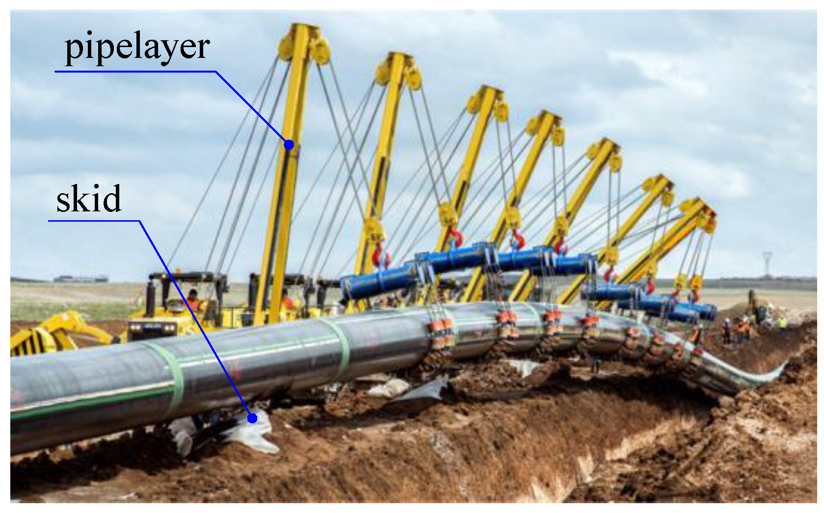
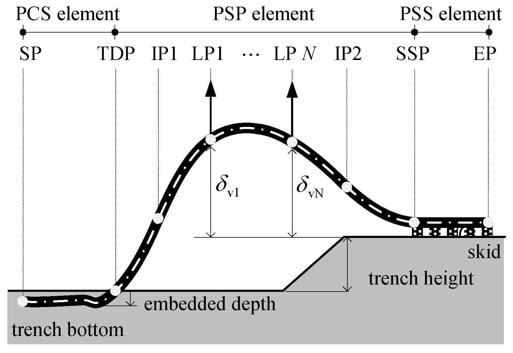
Figure 2 [21] shows the construction procedure of the lowering-in of a pipeline. The pipelayers lift the pipeline from the ground surface and pull it down on the centerline of the trench bottom. The gravity loads from the self-weight of the pipeline activate as a force to lower the pipeline into the trench. After one end of the pipeline is lowered into the trench, all the pipelayers subsequently drive along the pipeline at the same speed in the direction away from the lowered end, such that the remainder of the pipeline is lowered into the trench. This lowering-in subjects the pipeline to large deformations and bending loads, producing significant curvature between two zones of the pipeline, the above ground and the bottom of the trench zone [22].
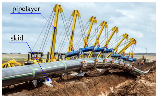
Figure 2.
Pipeline during lowering-in [21].
During this process, the pipeline experiences three-dimensional behavior with variable contact boundary conditions at the trench bottom. Therefore, to analyze the structural behaviors of the pipeline during lowering-in, the characteristics described above should be implemented in the analytical model. However, previous analytical models can consider specific loading points and deformations only, without reflecting variable loading and boundary conditions [2,3,4,5,6,7,8,9,10,11,12,13,14,15,16,17,18,19,20]. The 3-D behaviors of the pipeline can be simulated by superposition of the vertical plane (x-y plane) and lateral plane (x-z plane) behaviors. The pipeline in each plane can be partitioned into three zones: (i) contacting soil, (ii) supported by the skid and (iii) suspended by pipelayers. Herein, the geometry continuity and load transfer mechanism for each adjacent zone should be established. The torsional effects on the structural behavior of the pipeline during lowering-in were ignored. The axial forces applied to the pipeline were considered but the deformation corresponding to that forces was not considered. Also, axial forces are assumed to be consistently distributed over the entire pipeline.
For the zone contacting soil, the pipeline may be modeled as a Winkler foundation to simplify the pipeline-soil interaction. However, this model, which consists of independent discrete springs, fails to consider the interactions of adjacent spring elements and traction forces at the contact surface between the pipeline and soil. To clearly consider the pipeline and soil interaction, the pipeline contacted with soil can be modeled with a two-parameter beam on an elastic foundation (BOEF, [23,24,25,26,27,28,29,30]); in this study, pipeline model contacted with soil is referred to as a PCS (Pipeline Contacted with Soil) element.
For the zone supported by the skid placed on the ground along the sideline of the trench—as shown in Figure 2—the spacing of the skids is very small compared to the entire length of the pipeline. Consequently, the effect of the skid on the structural behavior of pipeline is negligible. Therefore, this zone is modeled as a series of springs with a single material property representing the skids. Thus, this model is effectively the same as the PCS element and is named a PSS (Pipeline Supported Skid) element. In the lowering-in phase, the lateral displacement of the pipeline is constrained to prevent the pipeline from leaving the skid and the centerline of the trench bottom. Therefore, the dislocations and deformations of the pipeline in the lateral plane are negligibly small in these zones. On the other hand, at the locations where the pipeline is separated from the skid and touches soil, the pipeline has a rotational angle in the lateral direction. Therefore, the pipeline in the lateral plane of both zones can be modeled as a rigid beam.
Finally, in the zone where the pipeline is suspended by pipelayers, discontinuity of the shear force is developed due to the pipelayer suspending forces and the inflection point appears due to the double bending moments. The pipeline is partitioned into several elements for each discontinuity and inflection point. Each element is modeled by a Euler-Bernoulli beam. These elements are named a PSP (Pipeline Suspended by Pipelayers) element.
2.2. Mathematical Formulations for Segmental Pipeline Models
The partitioned points and elements in the vertical plane are schematically shown in Figure 3. Here, SP(Start Point) and EP(End Point) are the starting and ending points of the pipeline, respectively. TDP(Touch Down Point) and SSP(Separated from Skid Point) indicate the points where the pipeline touches the soil and is separated from the skid, respectively.

Figure 3.
Segmental pipeline model in the vertical(x-y) plane.
LP1 through LPN are the lifting points by the pipelayers. Also, IP1 and IP2 are the inflection points of the pipeline. The PCS and PSS elements representing the pipeline contacted with soil and supported by a skid in the vertical plane are formulated by the following equation:
where is the constant load per unit length of the pipeline, is the soil stiffness in the vertical direction and is a constant traction on the laid pipeline. The two parameters of the foundation— and —are evaluated from the soil properties including the elastic modulus, , Poisson’s ratio, and vertical deformation parameter within the subsoil, , defined as and by Vlasov and Leont’ev formulations [30], respectively. Typically, the range of is from to [29]. For this reason, the was assumed to be in this study.
Upon solving the characteristic equation of Equation (1), there are three combinations of solutions depending on the relationship between and . Generally, is satisfied in most engineering problems [29,30], so that the behavior of PCS and PSS elements can be defined as follows:
where, , , and are integral constants,
, ,
, ,
, .
As in previous analytical models with two parameters, BOEF assumes that the boundary condition as semi-infinite. This condition provides a convenient calculation but has limitations when considering the separation length increase of the pipeline from the soil or skid. Thus, the semi-infinite boundary condition is invalid to reflect the beginning and final phase of lowering-in due to the small contact surface between the pipeline and the soil or skid. Therefore, a model of the shear layer is necessary to adequately consider the contact problem between the pipeline and the soil or skid beneath the lowering-in phase. The soil pressure applied to the pipeline is defined as in the PCS and PSS elements. The governing equation of the shear layer can be obtained by solving the homogeneous equation of the soil pressure. By substituting boundary conditions at (), the governing equation of the shear layer is as follows:
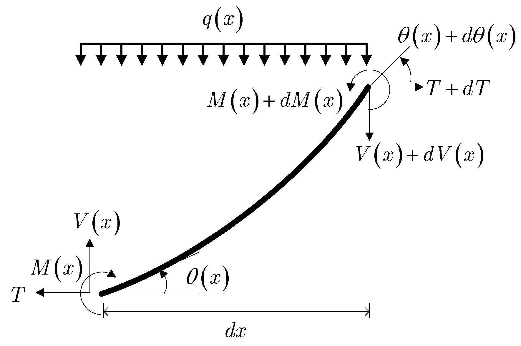
where and is an integral constant. The deflected infinitesimal element of the pipeline suspended by pipelayers (PSP element) in the vertical plane is shown in Figure 4. Using the equilibrium equations and the moment-curvature relationship, the PSP element is expressed by the following equation:
where is the vertical displacement of the pipeline, is the axial force applied to the pipeline and is defined in Equation (1). By solving Equation (4), the general solution can be obtained as follows:
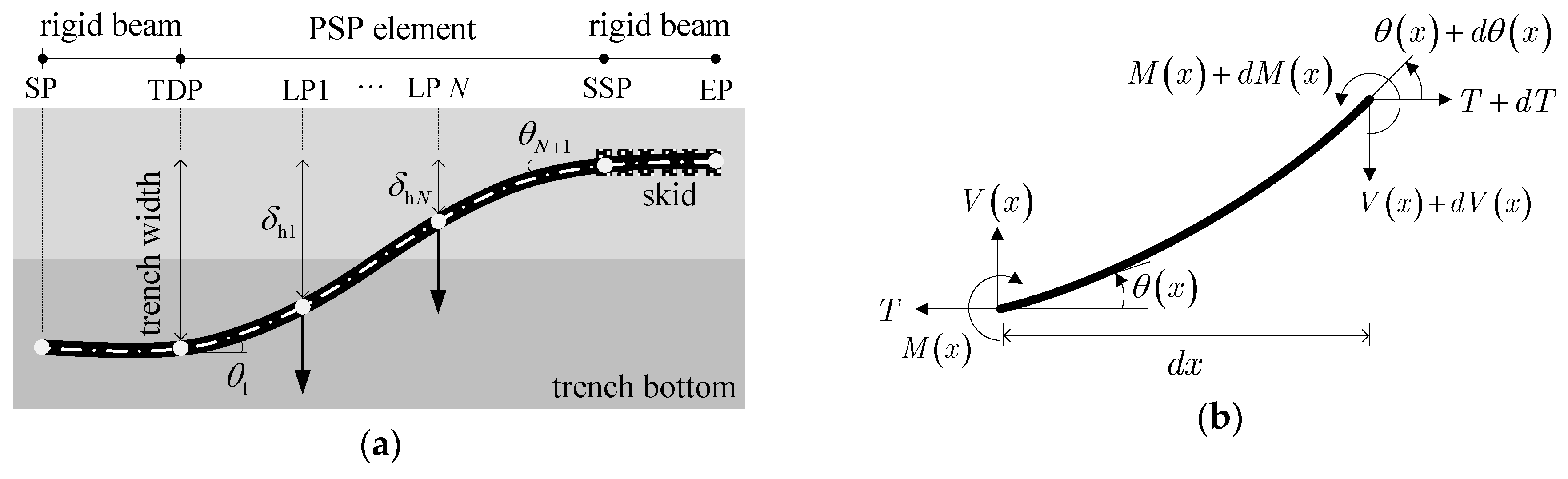
where , , and are integral constants. In the lateral plane, the pipeline suspended by the pipelayers is subjected to lateral displacement, as shown in Figure 5a. By applying the equilibrium equations and the moment-curvature relationship to the deflected element, as shown in Figure 5b, the governing equation of the PSP element can be expressed as follows.
where, is the lateral deflection of the pipeline, while the other parameters are the same as defined in Equation (4). is the axial force applied to the pipeline. The general solution corresponding to the PSP element for the lateral plane is shown in Equation (7).
where, is the same as that defined in Equation (5) and , , and are the integral constants. To analyze the structural behavior of the pipeline during lowering-in, the PCS, PSS and PSP elements are combined into segmental pipeline models, which are defined in Section 3.2. The three-dimensional (3-D) structural behavior of the pipeline can be implemented by superposing the segmental models in each plane. When the elements are combined, the geometry continuity at the boundaries between adjacent elements should be satisfied. However, the shear force discontinuities need to be considered at the lifting points of the pipelayers.

Figure 4.
Deflected infinitesimal element of a Euler-Bernoulli beam.

Figure 5.
Segmental pipeline model in the lateral (x-z) plane: (a) pipeline model using a pipeline suspended by pipelayers (PSP) model element; (b) deflected element of a Euler-Bernoulli beam.
3. Validation of Segmental Pipeline Models
3.1. Lowering-in Process and Configuration of Pipeline
Three phases in the entire lowering-in process can be considered: Phase (1) lifting the pipeline from the skid; Phase (2) laterally moving the lifted pipeline toward the trench; and Phase (3) lowering the pipeline into the trench bottom. Among the three phases, the phase that is investigated is first selected for use of the segmental pipeline model. Based on the specific phase, the pipeline is partitioned by considering the geometry and boundary conditions.
In Phase 1, the pipeline can be partitioned into PCS or PSS and PSP elements. The PSP element can be re-partitioned by considering the operations of the pipelayers such as the number of the pipelayers and their distances. In Phase 2 and Phase 3, the pipeline is divided into the vertical and lateral planes and both planes are superposed because the pipeline has a three-dimensional behavior. In the Phase 3 details, if the pipelayers are located around the central zone of the entire pipeline (TDP–SSP), both end regions (SP to TDP, SSP to EP) of the segmental pipeline model, where the pipeline contacts with soil and is supported by the skid, are modeled with PSS and PCS elements, respectively. The TDP to SSP region is modeled with a PSP element.
For all elements, the segmental length of each element in the vertical plane is unknown, except for the spacing between each pipelayer. These unknowns can be determined through the approach of the boundary value problems. In the lateral plane, the pipeline is modeled with a PSP element without inflection points due to the moment direction of the pipeline. The segmental length of the PSP element in the lateral plane is determined based on the segmental length of each element obtained in the vertical plane. The details of the segmental pipeline model for the lowering-in phase are addressed in the next section.
3.2. Model 1 and 2 for the Lowering-in Phase
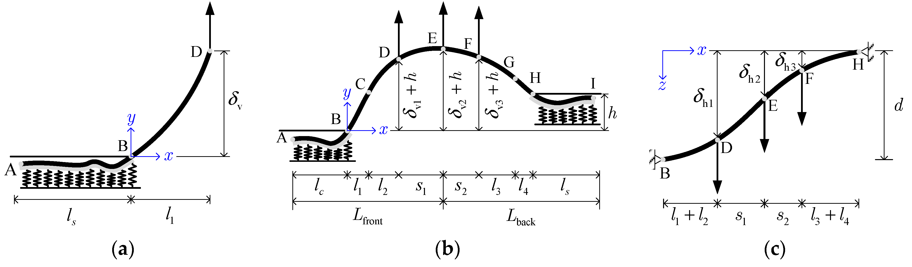
Model 1 and Model 2 depending on the configurations of the pipelayer are defined as shown in Figure 6a,b, respectively. Figure 6c shows the lateral plane of Model 2. Model 1 is composed of each single PSS and PSP element and it includes a shear layer in the PSS element. The solutions of Model 1 are presented in Equation (3).
where, is the deformation of the shear layer and and are the deformations of the PSS and PSP elements in the vertical plane, respectively. The entire length of the pipeline is known, while the segmental lengths of each element are unknowns. The unknown lengths and integral constants depending on the construction conditions can be obtained by using the following boundary conditions:
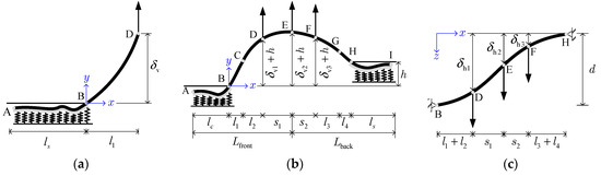
Figure 6.
Segmental pipeline model during lowering-in (a) Model 1; (b) Model 2; (c) lateral plane of Model 2 (A:SP, B:TDP, C:IP1, D:LP1, E:LP2, F:LP3, G:IP2, H:SSP, I:EP).
The integral constants are function of the segmental lengths, which are obtained by substituting Equation (9) except for the boundary condition of into Equation (8). Considering the total length of the pipeline, the segmental lengths presented in Figure 6 are determined by substituting the integral constants into the boundary condition of . The results are expressed with a system in Equation (10).
where, and are the length of each element for Model 1. This nonlinear algebraic system can be solved using the Newton-Raphson method and so forth.
Model 2 is defined in Figure 6b,c, which present the behavior of the vertical and lateral planes. If three pipelayers are applied, Model 2 has three discontinuity points of shear forces and two inflection points in the vertical plane and three discontinuity points of shear forces in lateral plane. Therefore, in the vertical plane, Model 2 is assembled with each single PSS and PCS element and six PSP elements. Thus, 10 equations for the vertical displacements of the elements including the shear layer are applied, as shown in Equation (11).
where, for the case of three pipelayers, and are the deflections of the shear layer, and are the deflections of the PCS and PSS element in the vertical plane, respectively. There are 34 integral constants and 6 unknown lengths (, , , , and ) in Equations (11). All unknown parameters can be obtained by applying the following boundary conditions:
As shown in Figure 6b, the lengths of SP to LP2 and LP2 to EP are and , respectively. Similar to Model 1, the boundary conditions except for the end displacements of each PSP element, which are , , and , are substituted into Equation (11). Then, the integral constants can be defined as a function of the segmental lengths of the elements. Through substituting these integral constants into the excepted boundary conditions, the nonlinear system related to the end displacements of the PSP elements is defined as shown in Equation (13).
In this equation, the integral constants – are functions of and and – are functions of , and . Also, the integral constants – are functions of , and . This nonlinear system can be solved with the Newton-Raphson method.
Model 2 in the lateral plane is assembled with four PSP elements if three pipelayers are applied. Thus, the 4 equations for the horizontal displacements of the elements are shown below.
The segmental length of each PSP element in the lateral plane can be determined by adopting the results of each element length calculated by Equation (13). The boundary conditions to obtain the integral constants in Equation (14) are defined in Equation (15).
Through the above processes, the sectional force of the segmental pipeline model can be evaluated using the elastic theory with and . Using the segmental pipeline model, the assessment for the 3-D behavior of a pipeline is performed on the sectional force and Von-Mises stress by root means square (RMS). Details for analyzing the Models 1 and 2 are included in Appendix A.
3.3. Finite Element Analysis for the Lowering-in Phase
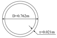
The segmental pipeline model for Models 1 and 2 was verified by finite element (FE) analysis using ABAQUS [31]. In the FE model, the pipeline is modeled with a 3-D beam element (B31) to simulate the bending behavior in the vertical and lateral plane. Also, the pipeline was assumed to behave in the elastic range. Its diameter and thickness were applied as 0.762 m and 0.021 m, respectively. The trench was modeled using 3-D shell elements (S4) and the geometry of the trench was determined considering the standard of SP 42-102-2004 [32] and the diameter of the pipeline. The deformable depth of a soil was assumed to be 1 m, considering the depth of the active layer and the freezing layer in common soil. This depth is reflected with the thickness of the shell element. The plastic behavior of the soil was ignored and considered as an elastic material. The material and geometric properties of the pipeline and trench are summarized in Table 1. The grade of the pipeline is X70 and considering the stiff soil condition, an elastic modulus and Poisson’s ratio were 40 MPa and 0.32, respectively. The skid had the same material properties as the trench and its height was the initial position of the pipeline. The pipelayers control the displacement only to support the pipeline. A general contact option in ABAQUS was used to implement the contact boundary condition between the pipeline and the trench. The general contact was applied to provide interactions such as traction on the surface between the pipeline and the trench. Before the lowering-in, the boundary conditions of displacement for the pipeline were free but the displacement on all sides of the trench was fixed. The pipeline was placed by self-weight at the top of trench, assumed as a skid and the general contact was accommodated between the pipeline and the trench. During lowering-in, the pipeline was lowered into the trench bottom by the displacement loads at the lifting point of pipelayers. In this process, the surfaces between the pipeline and trench contacted with each other were applied as general contact. A hard contact condition and friction coefficient of 0.3 were considered for the normal and tangential behaviors of the contact surfaces, respectively. Typically, the frictional coefficients between the steel and soil have a range of 0.14 to 0.26. To prevent slippage between the pipeline and the soil, the frictional coefficient of the soil used was as 0.3, which is slightly larger than typical values.

Table 1.
Material and geometric properties for the finite element (FE) models.
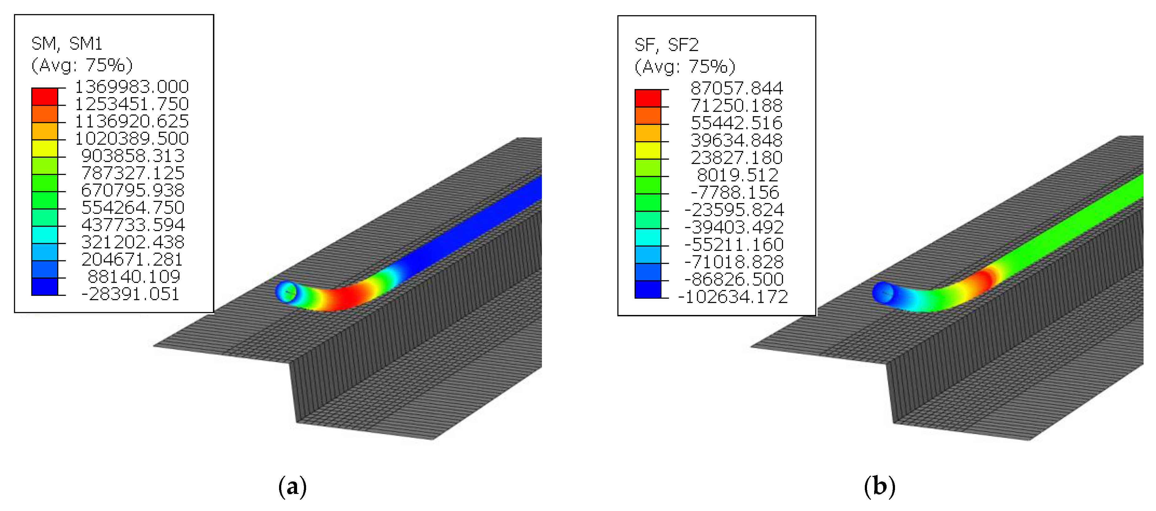
The static analysis was performed discretely for each phase of the lowering-in. The bending moments in the vertical and lateral plane were carried out from SM 1 and 2 in the output of Abaqus, respectively. Also, the output variables corresponding to the shear forces in the vertical and lateral plane are SF2 and 3. The results of FE analysis for Model 1 and Model 2 represented as shown in Figure 7.

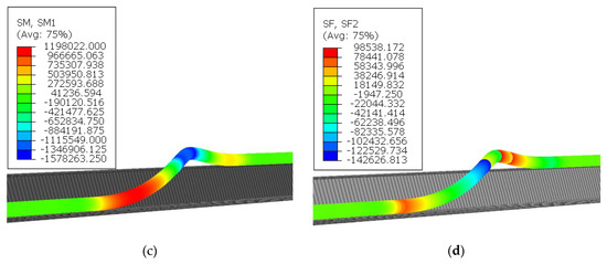
Figure 7.
Sectional forces of FE model (rendering contour): (a) bending moments for Model 1 (unit : N·m); (b) shear forces for Model 1 (unit : N); (c) bending moments for Model 2 (unit : N·m); (d) shear forces for Model 2 (unit : N).
3.4. Comparison of the Analytical and FE Analysis Results
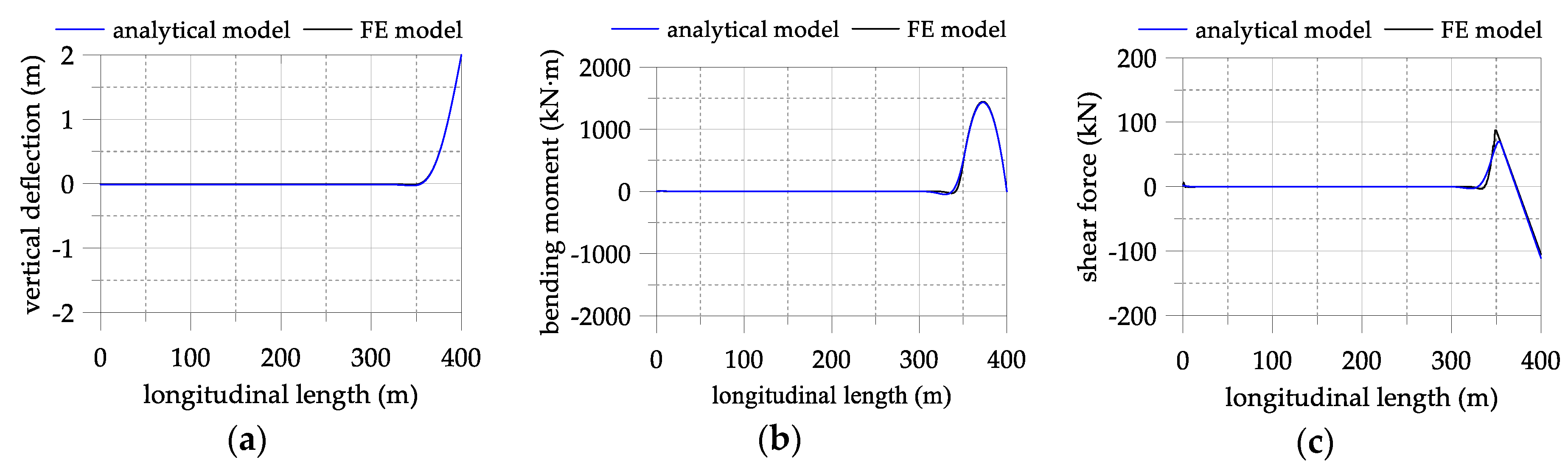
The analysis results for the vertical deflections, bending moments and shear forces of Model 1 are shown in Figure 8. Compared to the results of FE model, the deflections show good agreement, where the bending moments and shear forces are only slightly different near the TDP and SSP.
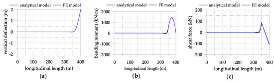
Figure 8.
Comparison of Model 1 to the FE analysis results during lowering-in: (a) deflection; (b) bending moment; (c) shear force.
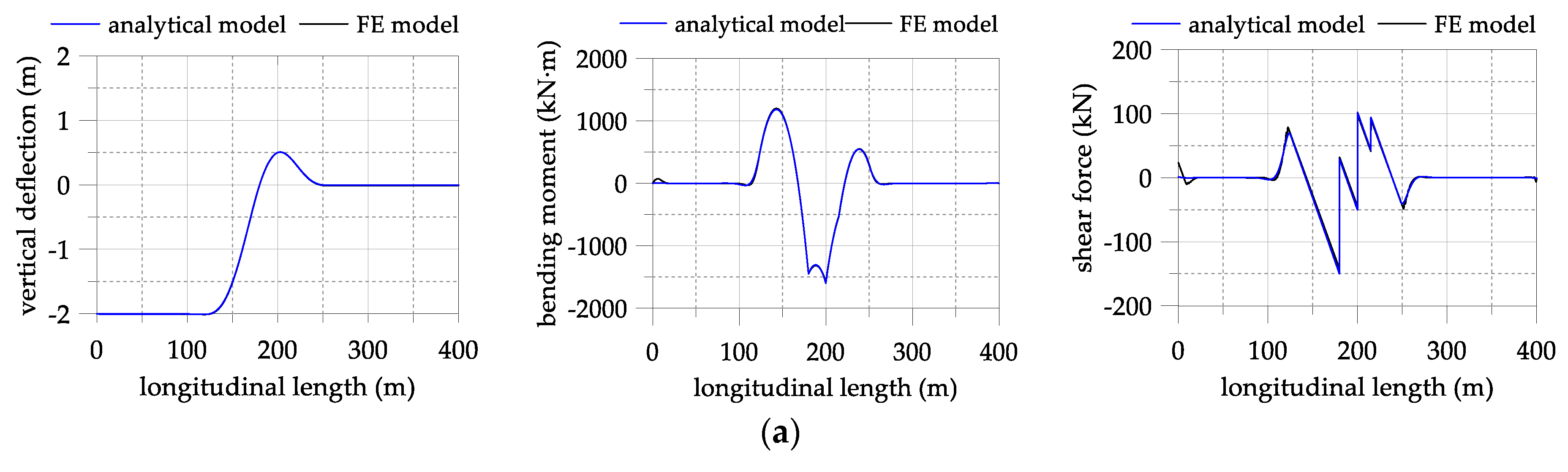
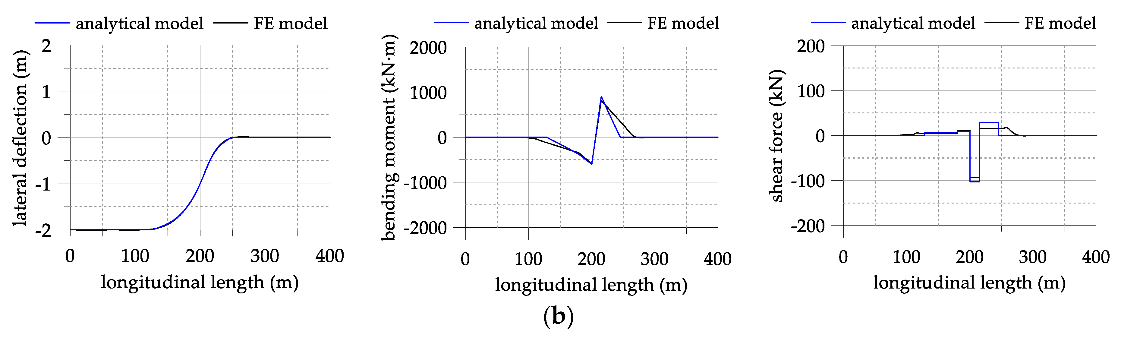
Figure 9a,b show the structural behavior of Model 2 compared to the FE model results. It should be noted that the analytical model provides better accuracy in the vertical plane than the lateral plane. For the lateral plane, the deformation of the pipeline is almost the same as in the FE analysis. However, the maximum and minimum bending moments and shear forces are somewhat different form the results of the FE analysis. Further, a difference appeared near the TDP and SSP.
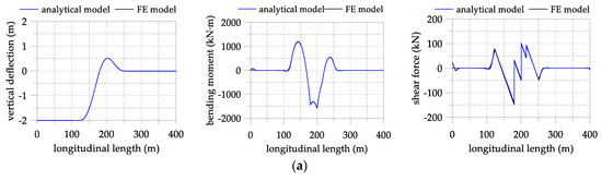
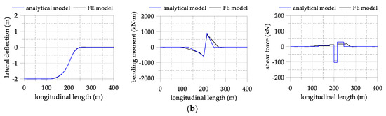
Figure 9.
Comparison of Model 2 to FE analysis results during lowering-in: (a) vertical plane (x-y plane); (b) lateral plane (x-z plane).
The segmental pipeline model simulates the interaction of the pipeline and the support layer (e.g. soil or skid) by applying vertical springs and shear layers. In the lateral plane, the TDP and SSP of the segmental pipeline model were simplified to pin-supported conditions and the pipeline supported by the skid and contacted with the soil was assumed to be a rigid beam. In addition, the effects of the soil and skid on the pipeline behavior in the lateral plane were assumed to be negligible. In the segmental pipeline model, the axial force of the pipeline was assumed to be constant and the deformation corresponding to the axial force was ignored. In contrast, for the FE analysis the interaction between the pipeline and the support layer was rigorously implemented by considering the material properties in addition to the normal and tangential behaviors of the contact surface. In particular, the TDP and SSP of the FE model were affected by the interaction between the trench and the pipeline in the lateral plane. Therefore, it seems that simple modeling of the interactions between the pipeline-trench and simplified boundary conditions of the segmental pipeline model lead to some difference, compared to the results of the FE analysis.
However, for the sectional force in the pipeline, the absolute value of the differences was very small compared to the overall values. Moreover, during lowering-in, the vertical displacement of the pipeline should be carefully controlled and investigated for structural safety. This means that the vertical plane behavior of the segmental pipeline model is more important and the model performance is dependent on the accuracy of the vertical plane results.
4. Application of the Segmental Pipeline Model
The number of pipelayers and their locations are key parameters to identifying the structural behavior of the pipeline during lowering-in. Equation (8) represents the vertical displacements of Model 1. Note that Model 1 simulates the pipeline behavior during the lifting construction sequence and it considers only one pipelayer. However, several pipelayers can be added in Model 1 to simulate different construction sequences, which are presented in Table 2. Case 1 considers two pipelayers during lifting construction sequence (Phase 1) and Case 2 considers three pipelayers for the same construction sequence of Case 1. Additionally, Case 3 considers three pipelayers and the construction sequence is the placing the pipeline down into the trench bottom, which is Phase 3 during lowering-in. In Case 3, the lateral behavior of the pipeline should be depicted. In Table 2, LP1 to LP3 are the first to third pipelayer and their locations are presented in Table 2. For Case 1, the segmental pipeline model is modeled with three PSP elements due to the presence of one inflection point and one additional lifting point. For Case 2, the segmental pipeline model is modeled with four PSP elements due to the additional lifting point compared to Case 1. For Case 3, the segmental pipeline model is modeled with six PSP elements due to one more inflection point, compared to Case 2. For all cases one PSS element is considered.
Table 2.
Case examples of the segmental pipeline model.
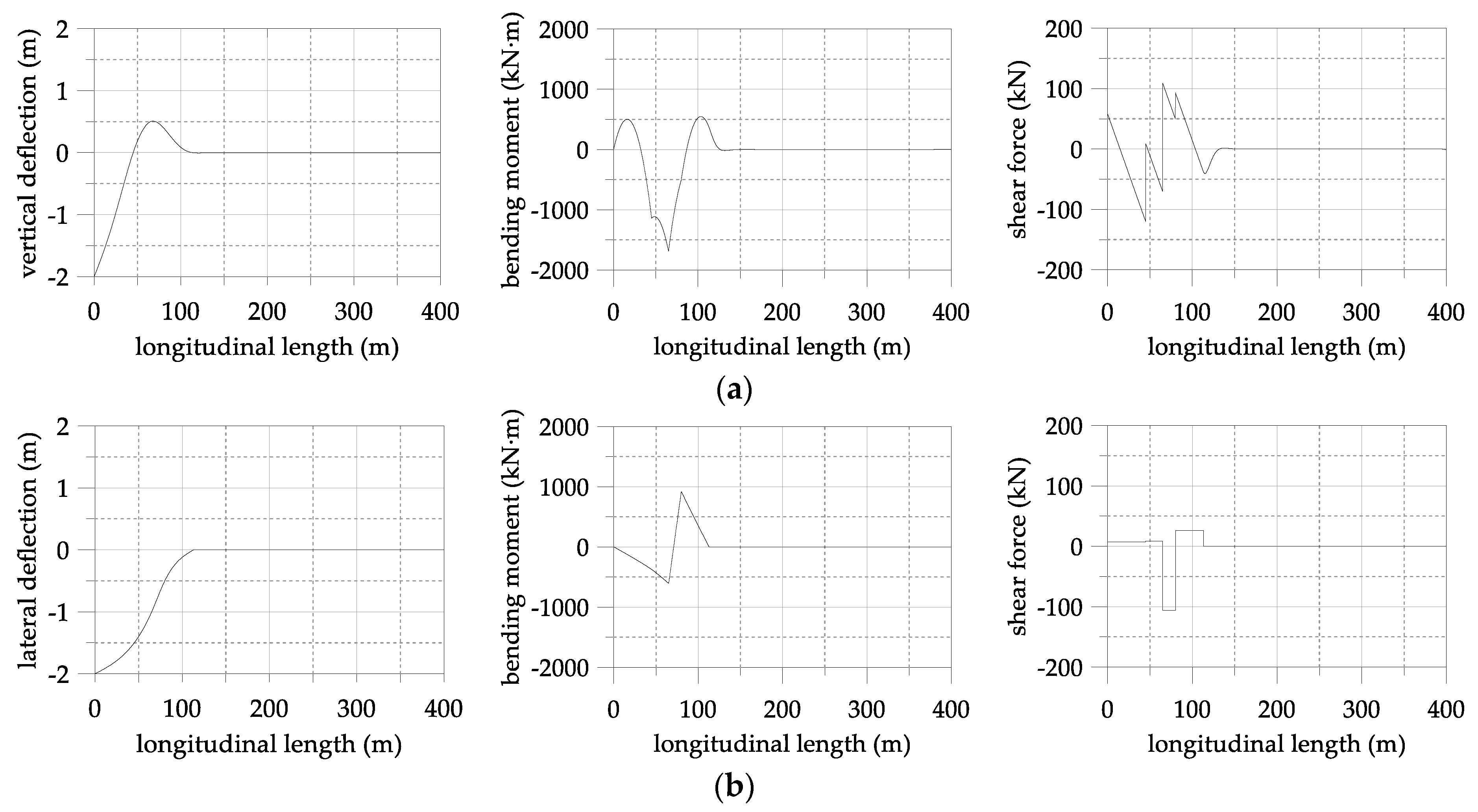
The analysis results for Case 1 and Case 2 are shown in Figure 10a,b, respectively. The zero-vertical deflection is the initial elevation of the skids. The vertical deflections remain negative up to about a pipeline length of 300 m and the amounts of the vertical deflections are almost identical to the initial deflections caused by the pipeline self-weight. For the range showing positive deflection values, the bending moment increases significantly but becomes zero at the final location of the pipelayers (for instance, LP2 for Case 1 and LP3 for Case 3). The maximum shear force resulting from Case 2 is slightly larger than for Case 1 but the difference is very small.
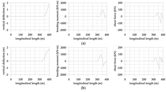
Figure 10.
Analysis results of the segmental pipeline model during lowering-in for (a) Case 1; (b) Case 2.
The sectional forces of Case 3 in the vertical plane are larger than those in the lateral plane, as shown in Figure 11. The ratios of the absolute maximum force for Case 1 to Case 2 are about 0.91 for the bending moment and 1.17 for the shear force, respectively. This shows that evaluation of the shear force is needed when the addition of a pipelayer is required for safety. The ratios of absolute maximum force in the lateral direction to the vertical direction are about 0.56 for the bending moment and 0.68 for the shear force, respectively. This indicates that it is necessary to evaluate the sectional forces of pipeline in the lateral direction as well to ensure safety under construction.
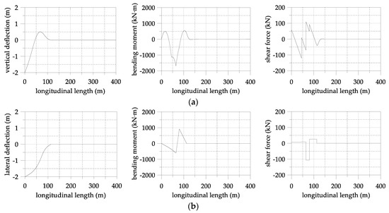
Figure 11.
Analysis results of Case 3: (a) vertical plane (x-y plane); (b) lateral plane (x-z plane).
The case examples show the extension of the segmental pipeline model with increasing pipelayers for both pipeline-lifting and putting construction sequences (lowering-in). In this extension process, it is convenient to build the segmental model by reflecting the locations of the pipelayers and adding proper elements corresponding to the boundary conditions.
5. Discussion
The load and boundary conditions applied to the pipeline which depend on the construction conditions during lowering-in are continuously changing. Therefore, to analyze the structural behavior of a pipeline, these characteristics should be considered. The previous analytical models are well established but they are limited with respect to formalized conditions such as the geometric, load and boundary conditions. The aims of the segmental pipeline model are to properly consider the formalized conditions, especially for the lowering-in conditions of a pipeline and to obtain numerical accuracy, applicability and convenience in the structural analysis. The segmental pipeline model was verified through FE analysis. In addition, assessment of the applicability and convenience was performed with 5 examples, including Models 1 and 2. The segmental model provides a good accuracy and can accommodate the construction features of lowering-in.
Torsions as well as bending moments are parameters that effect on the three-dimensional behavior of the pipeline. The proposed model and FE model, which based on the beam elements, are ignored the torsional effect on the structural behavior of pipeline. The pipeline-soil interaction of the FE model is implemented by the tangential and normal direction parameters in the surface between the pipeline and the soil as well as the material properties of the soil. Thus, the interaction between the pipeline and the soil, such as the lateral traction force, is considered in FE model. On the other hand, the pipeline-soil interaction of the segmental pipeline model is simplified to a vertical spring and shear layer with Vlasov and Leont’ev formulas. In addition, the proposed model was modeled without pipeline-soil interaction in the lateral plane. The pipeline of proposed model contacted with both the soil and skid in the lateral plane was assumed as a rigid beam. These rigid beams were not modeled in proposed model but the pipeline except for these rigid beams was modeled as Euler-Bernoulli beams. And then, the adjacent boundaries between the rigid beam and the Euler-Bernoulli beam (TDP and SSP in Figure 3) were pin-supported. In addition, the proposed model was assumed to have constant axial force in all cross sections. Such a simplification of the pipeline-soil interaction and lateral plane model lead to main difference from FE model.
The segmental pipeline model consists of PCS, PSS and PSP elements and each element can be combined to simulate various construction sequences in lowering-in. With these elements, the requirement of continuity in the geometry and sectional forces should be satisfied in the boundaries between each element. In the TDP and SSP positions, the segmental model has a small error in the sectional forces, compared to the FE analysis results. The error of the sectional forces is larger in the lateral plane than in the vertical plane. The boundary conditions suitable for the segmental model are limited to the translation and rotational displacements only. Also, the pipeline-soil interaction in the segmental model is simply considered with vertical springs and shear layers. If the limitation and simplification are implemented strictly into the model, the analysis results become more accurate. However, a rigorous model will be very complicated.
6. Conclusions
A segmental pipeline model was proposed to analyze the structural behavior of the pipeline during lowering-in, considering geometric and boundary conditions. The segmental pipeline model was formulated based on the two parameter BOEF and Euler-Bernoulli beam theory. The conclusions obtained from this study are as follows.
- The structural behavior resulting from the segmental pipeline model and the FE analysis showed good agreement, except for being slightly different in terms of the bending moments and shear forces near the TDP and SSP positions. The small difference is caused due to the limitation of applicable boundary conditions and simplification of the modeling of pipeline-soil interaction.
- During lowering-in, the boundary conditions of the pipeline are continuously changed due to the use of pipelayers. The segmental pipeline model can simulate variable boundary conditions, combining several PCS, PSP and PSS elements. This makes it more convenient to expand the segmental model to cover various construction sequences during lowering-in.
- The necessary elements in the modeling process can be intuitively selected by considering the geometric deformations and boundary conditions. The segmental pipeline model is built by combining the necessary elements and the final system equations of the segmental model are nonlinear, which can be solved easily through a numerical approach.
- The ratios of the absolute maximum bending moment and shear force in Case 2 to Case 1 were about 0.91 and about 1.17, respectively. Additionally, the ratios of the absolute maximum bending moment and shear force in the transverse direction to the vertical direction were about 0.56 and 0.68, respectively. This indicates that it is necessary to consider the sectional forces of pipeline in the lateral direction and the shear forces for an increase of pipelayers when analyzing the structural behavior of pipelines.
Author Contributions
Conceptualization, development of analytical model and verification, FE analysis, original draft preparation, data curation; W.H.; writing, review and editing, supervision, project administration, preparing the final version of this manuscript; J.S.L.
Funding
The National Research Foundation of Korea (NRF) grant funded by the Korean government grant number NRF-2017M2B2B1072890.
Acknowledgments
This work was supported by the National Research Foundation of Korea (NRF) grant funded by the Korean government (MSIP: Ministry of Science, ICT and Future Planning) (No. NRF-2017M2B2B1072890).
Conflicts of Interest
The authors declare no conflict of interest.
Appendix A
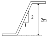
As shown in Figure A1, an example for segmental pipeline model is a lowering phase applied three pipelayers. Each of spacing between pipelayers is 20 m (LP1 to LP2) and 15 m (LP2 to LP3), respectively. The lifting heights at LP1, LP2 and LP3 measured from the trench bottom are assumed to be 2 m, 2.5 m and 2.4 m, respectively. Also, the height from the trench bottom to the skid is assumed to be 2 m.
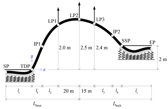
Figure A1.
Schematic representation of the lowering-in phase with 3 of pipelayers.
Figure A1.
Schematic representation of the lowering-in phase with 3 of pipelayers.
The equations for each element of the segmental pipeline model are summarized in Table A1. The material and geometric properties of the pipeline and trench are the same as in Table 1 in the Section 3.3. Also the variables in the equations for each element such as , , and are calculated according to the assumptions and model settings of this paper.
Table A1.
The equations for each element of the segmental pipeline model.
Table A1.
The equations for each element of the segmental pipeline model.
| Equations for Each Element | ||
|---|---|---|
| shear layer of PCS | ||
| SP to TDP | PCS | |
| TDP to IP1 | PSP 1 | |
| IP1 to LP1 | PSP 2 | |
| LP1 to LP2 | PSP 3 | |
| LP2 to LP3 | PSP 4 | |
| LP3 to IP2 | PSP 5 | |
| IP2 to SSP | PSP 6 | |
| SSP to EP | PSS | |
| shear layer of PSS | ||
In order to analyze behavior of pipeline in the vertical plane, the integral constants and unknown lengths of the equations for each element should be obtained firstly. The boundary conditions at the partitioning points to obtain the unknown variables are represented in Equation (A1).
By approaching the boundary value problem using equations for elements, summarized in Table A1 and Equation (A1), all integral constants can be obtained as a function of elemental lengths. The displacement of the PSP elements of LP1, LP2, LP3 and SSP to estimate the unknown variables can be obtained as follows.
Substituting the integral constants, which are the function of the elemental length, into Equation (A2) then the following nonlinear system is obtained:
Two additional equations are needed to calculate the unknown the elemental length of the segmental pipeline model. If the length of the pipeline from SP to LP 2 is defined as and the length from LP 2 to EP is defined as , the two additional equations required to solve Equation (A3) are obtained as follows.
A combination of Equations (A3) and (A4) yields a 6 by 6 nonlinear system, which can be solved with the Newton-Raphson method. The unknowns such as the elemental lengths and integral constants obtained through this calculation procedure are summarized in Table A2.
Table A2.
The unknown lengths of each element.
Table A2.
The unknown lengths of each element.
| Front Side of LP2 | Back Side of LP2 | ||
|---|---|---|---|
| elements | Length of elements | elements | Length of elements |
| PCS () | 128.249 m | PSP 4 () | 15 m |
| PSP 1 () | 39.606 m | PSP 5 () | 23.223 m |
| PSP 2 () | 12.145 m | PSP 6 () | 6.855 m |
| PSP 3 () | 20 m | PSS () | 154.922 m |
In the lateral plane, the pipeline contacted with the soil and supported by the skid is assumed to be a rigid beam. Also, since the pipeline does not have inflection point and is only partitioned at the lifting point of the pipelayer. Therefore, the pipeline in the lateral plane can be described as shown in Figure A2.
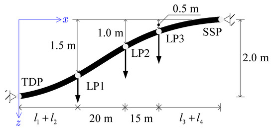
Figure A2.
Segmental pipeline model in the lateral plane with 3 pipelayers.
Figure A2.
Segmental pipeline model in the lateral plane with 3 pipelayers.
The locations of TDP, LP1, LP2, LP3 and SSP were assumed to be the same as both the vertical and lateral plane. Therefore, the elemental length of the model in the lateral plane can be calculated as the sum of and , the sum of and , respectively. The equations and lengths for each element are summarized in Table A3.
Table A3.
The equations for each element of the segmental pipeline model in the lateral plane.
Table A3.
The equations for each element of the segmental pipeline model in the lateral plane.
| Equations for Each Element | Elemental Length | ||
|---|---|---|---|
| TDP to LP1 | PSP 1 | 51.752 m | |
| LP1 to LP2 | PSP 2 | 20 m | |
| LP2 to LP3 | PSP 3 | 15 m | |
| LP3 to SSP | PSP 4 | 30.078 m | |
The integral constants of the equations for each element in Table A3 can be obtained by using the following boundary conditions.
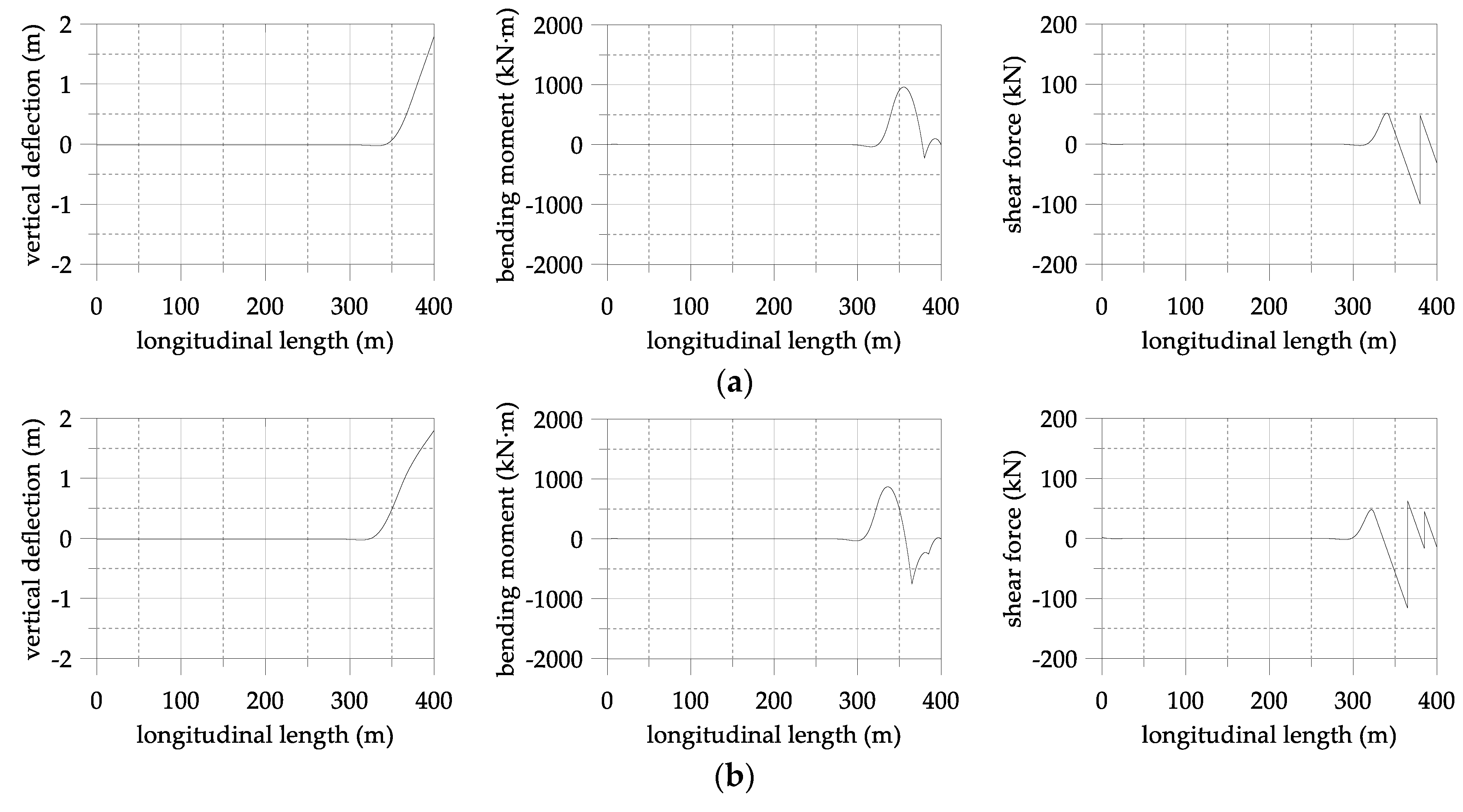
By substituting the integral constants obtained through the above procedure into the equations for each element, the behavior of the pipeline in the lateral plane can be analyzed. The sectional force of the segmental pipeline model can be evaluated using the elastic theory with and . Figure A3 and Figure A4 show the analysis result for the segmental pipeline model in the vertical plane and the lateral plane.
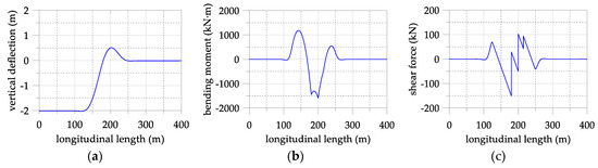
Figure A3.
Analysis results of the segmental pipeline model in the vertical plane: (a) deflections; (b) bending moments; (c) shear forces.
Figure A3.
Analysis results of the segmental pipeline model in the vertical plane: (a) deflections; (b) bending moments; (c) shear forces.
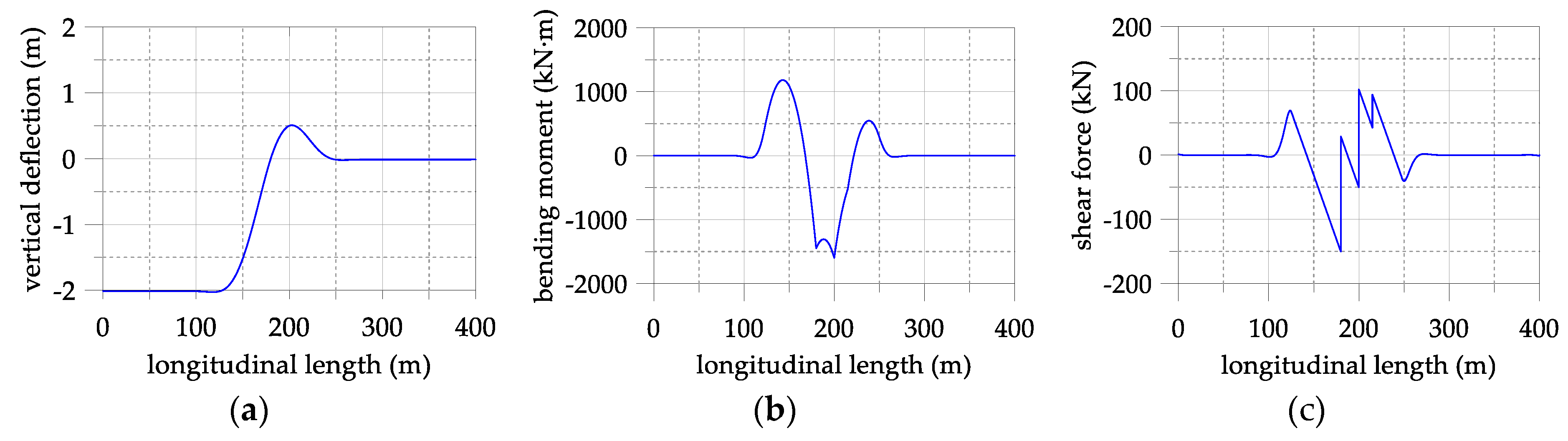
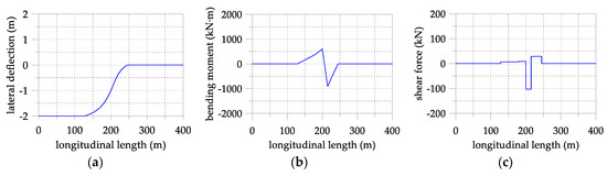
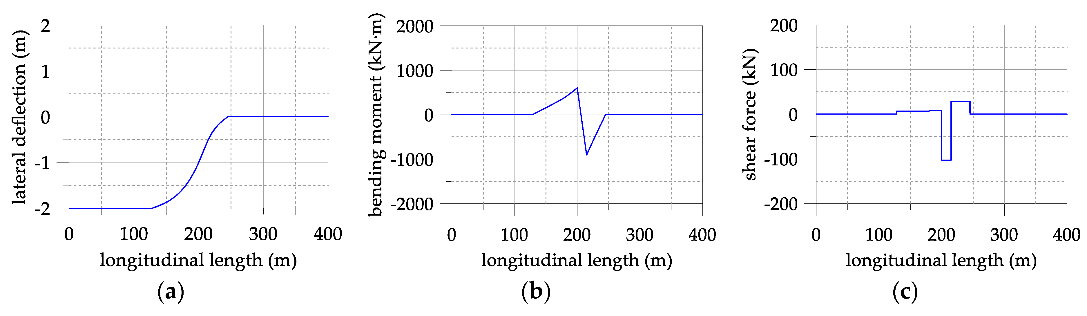
Figure A4.
Analysis results of the segmental pipeline model in the lateral plane: (a) deflections; (b) bending moments; (c) shear forces.
Figure A4.
Analysis results of the segmental pipeline model in the lateral plane: (a) deflections; (b) bending moments; (c) shear forces.
Using the segmental pipeline model, the assessment for the 3-D behavior of a pipeline is performed on the sectional force and Von-Mises stress by root means square (RMS). The 3-D deflections, sectional forces (bending moments and shear forces) obtained by using RMS and Von-Mises stress of segmental pipeline model are represented as shown in Figure A5.
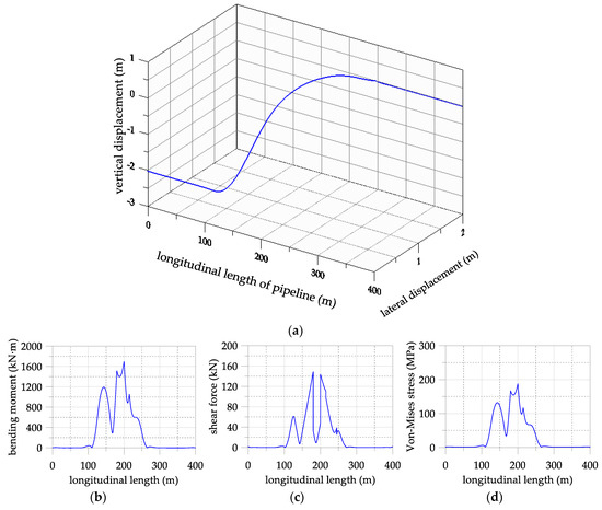
Figure A5.
The 3-D analysis results of the segmental pipeline model: (a) deflections; (b) bending moments obtained by using RMS; (c) shear forces obtained by using RMS; (d) Von-Mises stress.
Figure A5.
The 3-D analysis results of the segmental pipeline model: (a) deflections; (b) bending moments obtained by using RMS; (c) shear forces obtained by using RMS; (d) Von-Mises stress.
References
- Pipeline Research Council International, Inc. Best Practices in Applying API 1104 Appendix A; API Publishing Services: Washington, DC, USA, 2014. [Google Scholar]
- Scott, C.; Etheridge, B.; Vieth, P. An analysis of the stresses incurred in pipe during laying operations. In Proceedings of the 7th International Pipeline Conference (IPC 2008), Calgary, AB, Canada, 29 September–3 October 2008. [Google Scholar]
- Duan, D.M.; Jurca, T.; Zhou, C. A stress check procedure for pipe lowering-in process during pipeline construction. In Proceedings of the IPC, 10th International Pipeline Conference, Calgary, AB, Canada, 29 September–3 October 2014. [Google Scholar]
- Newmark, N.M.; Rosenblueth, E. Fundamentals of Earthquake Engineering; Prentice-Hall: Englewood Cliffs, NJ, USA, 1971. [Google Scholar]
- Hall, W.J.; Newmark, N.M. Seismic design criteria for pipelines and facilities, the current state of knowledge of lifeline Earthquake engineering. J. Struct. Eng. ASCE 1977, 103, 18–34. [Google Scholar]
- Wang, L.R.L.; O’Rourke, M.J.; Pikul, R.R. Seismic response behavior of buried pipelines. J. Press. Vessel Technol. ASME 1979, 101, 21–30. [Google Scholar] [CrossRef]
- Nelson, I.; Weidlinger, P. Dynamic seismic analysis of long segmented lifelines. J. Press. Vessel Technol. ASME 1979, 101, 10–20. [Google Scholar] [CrossRef]
- Muleski, G.E.; Ariman, T.; Aumen, C.P. A shell model for buried pipes in earthquakes. Int. J. Soil Dyn. Earthq. Eng. 1985, 4, 43–51. [Google Scholar] [CrossRef]
- O’Leary, P.M.; Datta, S.K. Dynamics of buried pipelines. Int. J. Soil Dyn. Earthq. Eng. 1985, 4, 151–159. [Google Scholar]
- Luco, J.E.; Barnes, F.C.P. Seismic response of cylindrical shell embedded in layered visco elastic half space. Earthq. Eng. Struct. Dyn. 1994, 23, 553–580. [Google Scholar] [CrossRef]
- Wong, K.C.; Shah, A.H.; Datta, S.K. Three dimensional motion of buried pipeline. J. Eng. Mech. ASME 1986, 112, 1319–1348. [Google Scholar] [CrossRef]
- Datta, S.K.; Shah, A.H.; Wong, K.C. Dynamic stresses and displacements in buried pipe. J. Eng. Mech. ASME 1984, 110, 1451–1465. [Google Scholar] [CrossRef]
- Takada, S.; Tanabe, K. Three dimensional seismic response analysis of buried continuous or jointed pipelines. J. Press. Vessel Technol. ASME 1987, 109, 80–87. [Google Scholar] [CrossRef]
- Lee, D.H.; Kim, B.H.; Lee, H.; Kong, J.S. Seismic behavior of a buried gas pipeline under earthquake excitations. Eng. Struct. 2009, 31, 1011–1023. [Google Scholar] [CrossRef]
- Kennedy, R.P.; Chow, A.W.; Williamson, R.A. Fault movement effects on buried oil pipeline. Transp. Eng. J. ASCE 1977, 103, 617–633. [Google Scholar]
- Wang, L.R.L.; Yeh, Y. A refined seismic analysis and design of buried pipeline for fault movement. Earthq. Eng. Struct. Dyn. 1985, 13, 75–96. [Google Scholar] [CrossRef]
- Karamitros, D.K.; Bouckovalas, G.D.; Kouretzis, G.P. Stress analysis of buried steel pipelines at strike-slip fault crossings. Soil Dyn. Earthq. Eng. 2007, 27, 200–211. [Google Scholar] [CrossRef]
- Trifonov, O.V.; Cherniy, V.P. A semi-analytical approach to a nonlinear stress–strain analysis of buried steel pipelines crossing active faults. Earthq. Eng. Struct. Dyn. 2010, 30, 1298–1308. [Google Scholar] [CrossRef]
- Dixon, D.A.; Rutledge, D.R. Stiffened catenary calculations in pipeline laying problem. J. Eng. Ind. ASME 1968, 90, 153–160. [Google Scholar] [CrossRef]
- Lenci, S.; Callegari, M. Simple analytical models for the J-lay problem. Acta Mech. 2005, 178, 23–39. [Google Scholar] [CrossRef]
- Maats Pipeline Professionals. Available online: https://www. maats.com/higher-lifting-capacity-roller-cradles (accessed on 3 December 2018).
- Sen, M.; Zhou, J. Evaluation of pipeline stresses during line lowering. In Proceedings of the 7th International Pipeline Conference (IPC 2008), Calgary, AB, Canada, 29 September–3 October 2008. [Google Scholar]
- Hetenyi, M. Beams on Elastic Foundation; University of Michigan Press: Ann Arbor, MI, USA, 1946. [Google Scholar]
- Filonenko-Borodich, M.M. Some Approximate Theories of the Elastic Foundation; No. 46; Uchenyie Zapiski Moskovskogo Gosudarstuennogo Universiteta Mechanika: Moscow, Russia, 1940; pp. 3–18. (In Russian) [Google Scholar]
- Pasternak, P.L. On a New Method of Analysis of an Elastic Foundation by Means of Two Foundation Constants; Gosudarsrvennoe Izdatelstvo Literaturi po Stroitelstvu i Arkhitekture: Moscow, Russia, 1954. (In Russian) [Google Scholar]
- Reissner, E. A note on deflection of plates on a viscoelastic foundation. J. Appl. Mech. 1958, 25, 144–145. [Google Scholar]
- Kerr, A.D. Elastic and viscoelastic foundation models. J. Appl. Mech. 1964, 31, 491–498. [Google Scholar] [CrossRef]
- Vlasov, V.Z.; Leont’ev, U.N. Beams, Plates and Shells on Elastic Foundations; Israel Program for Scientific Translation: Jerusalem, Israel, 1966; (Translated from Russian). [Google Scholar]
- Scott, R.F. Foundation Analysis; Prentice-Hall: Englewood Cliffs, NJ, USA, 1981. [Google Scholar]
- Zhaohua, F.; Cook, R.D. Beam element on two-parameter elastic foundations. J. Eng. Mech. ASCE 1986, 109, 1390–140220. [Google Scholar] [CrossRef]
- Simulia, D.S. Abaqus 6.16 Theory Manual; DS Simulia Corp: Providence, RI, USA, 2015. [Google Scholar]
- The Ministry of Fuel and Power Industry of the Russian Federation. Design and Construction of Gas Pipelines from Metal Pipes SP 42-102-2004; The Ministry of Fuel and Power Industry of the Russian Federation: Moscow, Russia, 2004.

© 2019 by the authors. Licensee MDPI, Basel, Switzerland. This article is an open access article distributed under the terms and conditions of the Creative Commons Attribution (CC BY) license (http://creativecommons.org/licenses/by/4.0/).