Article

A Probabilistic Hyperspectral Imagery Restoration Method

1
School of Computer Science, Northwestern Polytechnical University, Xi’an 710072, China
2
School of Electronic Engineering, Xidian University, Xi’an 710071, China
*
Author to whom correspondence should be addressed.
Appl. Sci. 2019, 9(12), 2529; https://doi.org/10.3390/app9122529
Submission received: 4 May 2019 / Revised: 10 June 2019 / Accepted: 19 June 2019 / Published: 21 June 2019
(This article belongs to the Special Issue Remote Sensing and Health Problems)

Abstract

:
Hyperspectral image (HSI) restoration is an important task of hyperspectral imagery processing, which aims to improve the performance of the subsequent HSI interpretation and applications. Considering HSI is always influenced by multiple factors—such as Gaussian noise, stripes, dead pixels, etc.—we propose an HSI-oriented probabilistic low-rank restoration method to address this problem. Specifically, we treat the expected clean HSI as a low-rank matrix. We assume the distribution of complex noise obeys a mixture of Gaussian distributions. Then, the HSI restoration problem is casted into solving the clean HSI from its counterpart with complex noise. In addition, considering the rank number need to be assigned manually for existing low-rank based HSI restoration method, we propose to automatically determine the rank number of the low-rank matrix by taking advantage of hyperspectral unmixing. Experimental results demonstrate HSI image can be well restored with the proposed method.

1. Introduction

Hyperspectral imagery (HSI) is 3D data containing both spatial and spectral information, which is widely used for lots of remote sensing related applications [1,2,3,4,5,6,7]. However, HSI is unavoidably influenced by multiple kinds of factors—including noise, stripe corruption, etc.—during imaging and acquisition [8], which decrease the image quality. Thus, it increases the difficulty for people interpretation or machine understanding [9,10,11,12], which makes HSI restoration an essential step for HSI processing and analysis.
To date, lots of methods have been proposed for HSI denoising. According to the way how noise and signal combines, typical HSI denoising methods can be categorized as signal-dependent-noise and signal-independent-noise methods. As indicated by the name, signal-independent-noise method assumes the generation of noise is independent of signals, while the generation of noise is related with signals for signal-dependent-noise method. These two kinds of methods are proposed for different HSI imaging mechanisms. For example, signal-independent-noise method is suitable to sensors where the noise is mainly determined by electronic components, while signal-dependent-noise method can be applied to the sensors where photon noise is dominated [13,14]. Both methods are research focuses of HSI denoising. Thus, lots of algorithms are proposed in recent years [11,13]. We mainly focus on signal-independent-noise method in this study. For signal-dependent-noise methods, we refer the readers to [13].
For signal-independent-noise HSI denoising methods, the existing focuses are original-space based methods, which includes total variation (TV) based, tensor based, local patch based, and low-rank based methods, etc. Low-rank based method has advantages to deal with missing data, which complies with the fact that HSI is also influenced by deadlines. Thus, low-rank based method has garnered significant attention in recent years for HSI denoising, which is also our focus in this paper. The detailed description of signal-independent-noise method is given in Section 2.
Though some low-rank based methods have been proposed, the following two deficiencies limit the usage of existing low-rank based methods. (1) In real applications, hyperspectral images will be influenced by multiple kinds of noise such as Gaussian noise, sparse noise, stripe, dead lines, and their combinations, which beyond the capability of the existing low-rank based methods. (2) The rank numbers of all existing low-rank based methods need to be assigned manually, and an automatic method to determine the rank number is desired.
To address those issues, we propose an HSI-oriented low-rank denoising method. Firstly, considering the mixture of Gaussian distribution has advantage of depicting different kinds of distributions, we propose to model noise with the mixture of Gaussian distributions. Thus, a probabilistic low-rank model is proposed for HSI denoising, where the clean HSI to be estimated is still considered as a low-rank matrix. Secondly, we find hyperspectral unmixing can provide prior information for rank number initialization. However, it is neglected by existing low-rank methods. In this paper, we propose to automatically determine the rank number via hyperspectral unmixing. In summary, the proposed HSI-oriented low-rank denoising method can deal with multiple kinds of noise as well as automatically determine the rank number. As a result, the proposed method has better HSI restoration results compared with other methods. Experimental results on both simulated and real datasets verify the effectiveness of the proposed method.
The paper is structured as follows. In Section 2, we briefly review the related work of HSI denoising. In Section 3, we analyze how to cast HSI denoising into a low rank matrix analysis (LRMA) problem and discuss how to initialize the rank number. In Section 4, we present the probabilistic low-rank based HSI restoration method. In Section 5, the experimental setup and results are summarized. Finally, we discuss the proposed method and conclude the paper in Section 6 and Section 7.

2. Related Work

We mainly focus on HSI denoising method where noise is independent with signal. The related works can be roughly divided into a transformation-space based method and an original-space based one [15,16].
Transformation-space based method is adopted for HSI denoising in the early stage. The basic idea of transformation-space based method is that the signal differs from the noise greatly when we transform the HSI from spatial/spectral space into a new space. For example, in the wavelet transformation space, the signal is sparse while the noise is non-sparse. Thus, signal can be separated from the noise by exploiting such difference. [17,18,19]. Except wavelet transformation, other transformation methods such as curvelet [20,21] can also be used for this purpose. The advantage of transformation-based method is that it does not need to assign noise a specific category (e.g., Gaussian noise). However, artifacts such as edge ringing and low-frequency noise are prone to be generated when using transformation-space based methods [16].
In contrast, original-space (image space or spectral space) based methods denoise HSI directly on spatial/spectral space. Since those methods do not influenced by artifacts and low-frequency noise, they begin to the dominate HSI denoising methods in recent years.
Considering the HSI image is a data cube composing a set of 2D band images, a direct strategy for original-space based method is to denoise each band image independently, which promotes some 2D denoising method directly used for hyperspectral image denoising. However, HSI contains both spatial and spectral information. Directly using 2D denoising methods for each band neglects the correlation among images from different bands. Thus, one trend of the original-space based method is to utilize both spectral and spatial information. Among those methods, total variation (TV) based [22,23,24], tensor based [25,26,27], local patch based methods, and low-rank based methods are representative approaches.
For TV based methods, considering the variations among neighboring pixels or spectra are smooth, TV based HSI denoising methods are proposed by exploiting such kind of smoothness [22,23,24]. Since the noise intensity of different bands may differ, spectral–spatial TV based methods consider the spectral noise differences as well as the spatial information differences simultaneously [24]. Considering HSI is a 3D data which can be naturally represented by 3D tensor, some tensor-based methods are proposed accordingly. It is noticeable that commonly used tensor decomposition strategy includes Tucker decomposition and PARAFAC decomposition [25,26,27]. For local patch-based method, it first divides HSI into a group of overlapping (or non-overlapping) 2D patches or 3D blocks, and then generates noiseless 2D patches or 3D blocks using collaborative filtering. Finally, it assembles those denoised 2D patches or 3D blocks to obtain the desired HIS [28,29,30,31]. Among which, video block-matching and 3D filtering (VBM3D) is a representative local patch/voxel based method. Though the advantages of above introduced spectral–spatial TV based, tensor based and local patch-based methods have been testified over traditional 2D approaches for HSI denoising, it is found that those methods are proposed for complete HSI data. If the HSI is incomplete—e.g., dead lines or dead pixels appear in HSI—the above methods cannot generate a complete HSI and their restoration results will be influenced greatly.
In recent years, low-rank based methods have been proposed for HSI denoising, which have the merit to deal with incomplete data. The representative method is a LRMA method [11], which assumes clean HSI is a low-rank matrix. Then, HSI restoration problem cast into recovering low-rank matrix from original noisy HSI data, which is solved by Go Decomposition (Godec) approach [11]. Based on [11], some other low-rank based methods are proposed by utilizing other characteristics of HSI for denoising. He et al. combine the TV-regularization term with low-rank matrix representation [32]. Wang et al. combine the non-local similarity with LRMR and thus proposed a method named group low-rank representation [33]. Superpixel segmentation is used together with low-rank representation to improve the performance of image denoising results [34]. Wei et al. propose a structured low-rank representation, which achieves the state-of-the-art denoising performance by utilizing the structure among low-rank matrix [35].
Though these low-rank based methods have been proposed, two deficiencies limit the their usage. 1) In real applications, hyperspectral image will be influenced by multiple kinds of noise such as Gaussian noise, sparse noise, stripe, dead lines, and their combinations. However, above mentioned methods model noise deterministically, which can only handle one to two kinds of noise and lose flexibility to handle complex noise. 2) The rank number of all existing low-rank based method need to be assigned manually, and automatically method to determine the rank number is desired. To deal with these two problems, we propose a new HSI-oriented denoising method in this paper.

3. Revisited Low-Rank based HSI Denoising from Linear Mixed Model Perspective

In this study, noisy HSI is denoted as X R n r × n c × n b . n r , n c , and n b represent the height, width, and bands of X , respectively. By vectorizing the image of each band of X we obtain a 2D matrix X R n b × n p , where n p = n r × n c denotes the number of pixels. In X , each row represents the spectrum of one pixel, while each column denotes the reflectance values of all pixels in one specific spectral band.
Suppose a noisy image X is consisted of a clean/noise-free image L R n b × n p and multiple kinds of noise S R n b × n p , i.e.,
X = L + S ,
HSI restoration is to recover L from X .
Due to the low spatial resolution and materials mixture in remote sensing, the spectrum of each pixel is always considered as the mixture of some spectral signatures of pure materials. The spectral signatures of pure materials are termed as endmembers, while the proportion of each endmember for mixing is termed as abundance. Thus, L can be decomposed into endmembers with an abundance matrix as
L = M H T ,
where M R n b × n e is an endmember matrix, H R n p × n e is an abundance matrix and n e is the number of endmembers. Figure 1 illustrates above representation. Based on the abovementioned issues, we first analyze why HSI denoising can be formulated as a LRMA problem. Then, we analyze how to use the provided prior knowledge LMM to initialize the rank number of LRMA.

3.1. Analyze HSI Restoration as a LRMA Problem

We use rank(•) to denote the rank number of a given matrix. It is realized that noise, i.e. r a n k ( S ) , is always a full matrix [29]. Since the row and column dimensionalities of S are n p and n b , r a n k ( S ) = min ( n b , n p ) .
Since L = M H T , the rank of noise-free HSI L , denoted as r a n k ( L ) , is min ( r a n k ( M ) , r a n k ( H ) ) . n e represents the number of endmembers, which is related with the materials captured in the HSI image. Since there are always several materials in the HSI image [29], n e is far smaller than the number of spectral bands n b or n p , which is always more than one hundred or ten thousand for an HSI image. Thus, r a n k ( L ) min ( r a n k ( M ) , r a n k ( H ) ) n e .
The rank of X , denoted as r a n k ( X ) , is no larger than r a n k ( L ) + r a n k ( S ) since X = L + S . According to the fact that n e is far smaller than n p and n b , r a n k ( L ) « min ( n p , n b ) = r a n k ( S ) , which makes r a n k ( L ) « r a n k ( X ) r a n k ( S ) .
According to above analysis and the fact that only several endmembers are always contained in one HSI in reality [29], HSI denoising can be casted into recovery a low-rank matrix L from X .

3.2. Analysis on the Rank Initialization for LRMA

Zhang et al. [11] first use the LRMA model for HSI restoration, which divides HSI into some fixed-size subcubes, then adopt LRMA method to restore each subcube and assemble those restored subcubes to obtain the final result. Rank number is manually initialized as the same value in [11] for each subcube. Though this kind of initialization is simple, it ignores the rank difference among different fixed-size subcubes in HSI. In other words, because the materials/endmembers falling into a fixed-size subcube are related with its content, the number of endmembers is always varied with different subcubes. Thus, the rank number should be varied according to r a n k ( L ) n e to fit the data better. However, this characteristic has not been considered in [11] and its follow-up methods.
Based on the data structure of HSI, we analyze and find two kinds of rank number initialization methods. Taking advantage of the number of endmembers, n e is an apparent clue/(prior knowledge) for rank number initialization. The first method is a whole HSI entity-based method, i.e., all pixels in HSI are used to estimate the rank number. The second method is a local region-based method. Similar to Zhang et al in [11], homogeneous regions are adopted instead of using fixed-size subcubes [11].
(1) Initialize the rank number using whole HSI entity
Since determining the number of endmembers in HSI is an important issue for hyperspectral unmixing, the relative methods can be directly introduced for rank number initialization. Without dividing HSI into some subcubes as Zhang et al in [11] does, those methods are based on all pixels in HSI. The reason using all pixels to determine the number of endmembers is partially because the parameters of those methods can be estimated more accurately with more pixels. Thus, we use whole HSI entity to estimate the number of endmembers, and then use the estimated number to initialize the rank number.
Information theoretic criteria including Akaike’s information criterion, minimum description length can be used to determine the number of endmembers, which is based on the data log-likelihood [35,36,37]. However, the prior knowledge of data log-likelihood function needs to be provided. Incorrect prior knowledge will influence the accuracy of estimated number of endmembers. On the contrary, geometry-based approaches can estimate the number of endmembers without knowing the prior knowledge of likelihood function. GENE-AH [38], a typical geometry-based approach, was proposed to estimate the number of endmembers. Since it assumes the observed pixels lie in the affine hull of endmembers, GENE-AH has an advantage in estimating the number of endmembers in the presence of noise, which promotes adopting GENE-AH to estimate the number of endmembers in this study.
(2) Initialize the rank number with homogeneous regions in HSI
Dividing HSI into fixed-size subcubes will lead to variation of the rank number with different subcubes [11]. Thus, assigning each subcube the same rank number is inappropriate. However, from the perspective of segmentation, an image can be divided into many of homogeneous regions. For hyperspectral image, the rank of the homogeneous region approximately equals to one because those homogeneous regions are always defined as the combination of pixels with similar spectral. It motivates us first segment/over-segment HSI into some local regions, then restore those local regions with LRMA method.

4. Probabilistic LRMA Model for HSI Restoration

From above analysis, we can see that HSI restoration is to estimate low-rank matrix L from X inversely in Equation (1). In this section, we first introduce how traditional methods estimate L from X , and then give the details of how we solve this problem with the probabilistic model.
Without any prior knowledge on S , estimating L from X is ill-posed. Certain constraints or priors on S are then needed to make L efficiently solvable. The original LRMA model assumes L and S are low-rank matrix and sparse matrix, respectively, with which the estimation of L is modeled as
min L , S r a n k ( L ) + λ S 0 s . t .    X = L + S .
The above formula is a nonlinear optimization problem, which is hard to solve. To make it tractable optimized, Formula (3) is converted into
min L , S L + λ S 1 s . t .    X = L + S
by replacing L0 norm with L1 norm and replacing the rank with the nuclear norm. λ is a weight to balance the importance of L and S [39,40].
Though the original LRMA model is suitable for incomplete data restoration, from the constraint on S , we can see that the original LRMA model is only suitable for noise in a sparse form.
However, the degradation factors such as multiple kinds of noise, stripe corruption, and missing data coexist in HSI, among which only few kinds of noise are sparse. This characteristic makes Equation (4) inappropriate to represent such kind of degradation in reality. In [11], the LRMA model is remodeled as
X = L + S + N ,
where the new supplemented item N is a Gaussian-distributed noise. Then, L can be solved by
min L , S L + λ S 1 s . t .    X L S F δ ,
where δ is a constant [41].
Though [11] can deal with more kinds of noise by dividing the noise item into S and N , from Equation (6) we can see the noise that [11] can essentially deal with is only Gaussian noise, sparse noise, and their combinations, which is still insufficient for real applications.

4.1. Framework

Since modeling noise deterministically as Equation (1) or Equation (2) can only represent some kinds of noise, we propose to model noise probabilistically. The basic assumption is that though S is difficult to be modeled deterministically for multiple kinds of noise, it will be easier and more flexible to be modeled from the probabilistic perspective. In addition, we can further initialize the rank number by taking advantage of the linearly mixed model, as we analyzed in Section 3. With these considerations, we propose a probabilistic LRMA based HSI restoration method, whose framework is shown in Figure 2.
It is commonly realized that mixture of Gaussian distribution can depict any continuous distribution. Thus, we probabilistically model noise S in HSI with mixture of Gaussian as
s i j k = 1 K ω k N ( s i j | μ k , τ k 1 ) .
s i j is the value in the j-th column and i-th row of S . K represents the number of Gaussian components. Given the mean value μ and precision τ as μ = μ k and τ = τ k , respectively, N ( s i j | μ k , τ k 1 ) depicts the adopted k-th Gaussian distribution. ω k is the mixing proportion weight which satisfies ω k 0 and k = 1 K ω k = 1 .
With such representation for S , likelihood between X and L obeys
p ( X | L , ω , μ , τ ) = ( i , j ) Ω ( k = 1 K ω k N ( x i j | l i j + μ k , τ k 1 ) ) ,
where l i j and x i j represent the element in the i-th row and the j-th column of L and X , respectively. Since K Gaussian distributions are adopted, ω = ( ω 1 , ω 2 , , ω K ) has K elements. Similarly, the mean value μ = ( μ 1 , μ 2 , , μ K ) and the precision value τ = ( τ 1 , τ 2 , , τ K ) also have K elements. ( i , j ) Ω is a subset composed by all possible values of ( i , j ) .
Denote θ as the parameter which controls the distribution of L R n b × n p . Choosing proper distribution and parameter θ can guarantee that p ( L | θ ) is a low-rank matrix [42,43]. For a probabilistic LRMA model, if ω , μ , τ , and θ are known in advance, restoration task turns to recover L from X as
L opt = arg max L p ( L | X ) p ( X | L , ω , μ , τ ) p ( L | θ ) .
However, ω , μ , τ and θ are all unknown in reality. To make those parameters data-dependent, they need to be estimated jointly with L as p ( L , ω , μ , τ , θ | X ) , which can be seen from Section 4.2.

4.2. Clean HSI Estimation Method

Considering matrix decomposition has the advantage to represent a low-rank matrix both in speed and scalability, it can be adopted to represent L . Specifically,
L = M H T = r = 1 R m . r h . r T .
The r-th column of M and H is denoted as m . r and h . r , respectively. θ = ( θ 1 , θ 2 , , θ R ) is precision parameter. To guarantee the generated matrix L a low-rank matrix, M and H can be probabilistically represented by Gaussian distributions [42] as
p ( M | θ ) r = 1 R N ( m . r | 0 , θ r 1 I n b ) p ( H | θ ) r = 1 R N ( h . r | 0 , θ r 1 I n p )
where I n p is an identity matrix in the size of n p × n p . θ r obeys Gamma distribution with hyperparameters a 0 and b 0 , viz. p ( θ r ) = Gamma ( θ r | a 0 , b 0 ) . With such a matrix decomposition L = M H T , p ( X | L , ω , μ , τ ) in Equation (9) turns to be
p ( X | M , H , ω , μ , τ ) = ( i , j ) Ω ( k = 1 K ω k N ( x i j | m i . h j . T + μ k , τ k 1 ) ) ,
and p ( L , ω , μ , τ , θ | X ) turns to be p ( M , H , ω , μ , τ , θ | X ) . It means instead of estimating L directly, we need to estimate M and H first, and then obtain L using L = M H T .
According to the Bayesian rule, p ( M , H , ω , μ , τ , θ | X ) is proportional to p ( M , H , ω , μ , τ , θ , X ) , which can be further factorized into some simple distributions to guarantee the easier estimation from the perspective of generative model. The above analysis on p ( M , H , ω , μ , τ , θ | X ) can be represented by
p ( M , H , ω , μ , τ , θ | X ) p ( M , H , ω , μ , τ , θ , X ) = p ( X | M , H , ω , μ , τ ) p ( ω ) p ( μ | τ ) p ( τ ) p ( M | θ ) p ( H | θ ) p ( θ )
Though the factorized items such as p ( M | θ ) and p ( H | θ ) , etc., can facilitate the estimation of unknown parameters { M , H , ω , μ , τ , θ } , directly estimating M and H using p ( M , H , ω , μ , τ , θ , X ) is still intractable. To address this problem effectively, variational method or sampling-based method can be used to calculate M and H . In this study, the variational method proposed in [42] is used for this purpose. The basic idea of this method is given as follows.
First, an intermediate variable t i j = ( t i j 1 , , t i j K ) { 0 , 1 } K , which satisfies a multinomial distribution parameterized by ω , is introduced to represent S as
s i j k = 1 K N ( s i j | μ k , τ k 1 ) t i j k .
Second, to guarantee Equation (12) tractable, we represent μ k , τ k and ω using the following conjugate priors
p ( τ k ) Gam ( τ k | c 0 , d 0 ) p ( μ k ) N ( μ k | μ 0 , ( β 0 τ k ) 1 ) p ( ω ) Dir ( ω | α 0 )
where c 0 , d 0 , and α 0 = ( α 01 , , α 0 K ) are the parameters of above distributions [42].
With above representations, we build a full probabilistic low-rank model, which is tractable. Thus, the estimated parameters are transformed into { M , H , t , ω , μ , τ , θ } from { M , H , ω , μ , τ , θ } , where t = { t i j } . For simplicity, we use Θ to denote all variables of { M , H , t , ω , μ , τ , θ } in the following.
Third, a new simple distribution q ( Θ ) is introduced to approximate p ( Θ | X ) as
KL ( q | | p ) = q ( Θ ) ln { p ( Θ | X ) q ( Θ ) } d Θ ,
where KL ( q | | p ) denotes the KL divergence between q ( Θ ) and p ( Θ | X ) . Since minimizing KL divergence between q ( Θ ) and p ( Θ | X ) can guarantee the estimation of Θ from q ( Θ ) is close to the one learned from p ( Θ | X ) , we estimate M , H together with other parameters by minimizing KL ( q | | p ) iteratively. The details can be seen from [42]. Here we only give the updating equation for m i . (the i-th row of M ) and h j . (the j-th row of H ). By defining q ( m i . ) = N ( m i . | μ m i . , Σ m i . ) and q ( h j . ) = N ( h j . | μ h j . , Σ h j . ) , the parameters related with m i . and h j . can be inferred. μ m i . T = Σ m i . { k τ k j t i j k ( x i j μ k ) h j } T and μ h j . T = Σ h j . { k τ k i t i j k ( x i j μ k ) m i } T are the mean vectors for m i . and h j . , while Σ m i . = { k τ k j t i j k h j T h j + Γ } 1 and Σ h j . = { k τ k i t i j k m i T m i + Γ } 1 are the covariance matrices for m i . and h j . . Γ = diag ( θ ) .
When the stop criterion is satisfied, the optimized m i . and h j . are denoted as m i . and h j . . Then each element in the denoised HSI image L can be calculated by l i j = m i . × ( h j . ) T .

4.3. Initialization of the Rank Number

Though the above introduced probabilistic low-rank method can represent the complex noise with the mixture of Gaussian strategy, one of the most important parameters, rank number R , has to be assigned manually. Fortunately, as we analyzed in Section 3, the number of endmembers n e can be used to determine R . Thus, we use an affine hull based method (named as GENE-AH [38]) to estimate the number of endmembers in this study, which can be used to initialize the rank number.
Suppose HSI X R n b × n p has n p pixels. Each pixel is denoted as x n R n b , where 1 n n p . It is assumed that the spectral of all pixels lie in an affine hull for GENE-AH method. We denote the estimated noise covariance matrix as D ^ N c . The parameter of affine set fitting parameter ( d ^ A f , C ^ A f ) can be represented by
d ^ A f = 1 n p n = 1 n p x n ,   C ^ A f = [ q 1 ( A f ) ( U A f U A f T n p D ^ N c ) , , q N max 1 ( A f ) ( U A f U A f T n p D ^ N c ) ] .
U A f = [ x 1 d ^ A f , , x n p d ^ A f ] R n b × n p is the mean removed data matrix, q i ( A f ) ( U A f U A f T n p D ^ N c ) represents the unit-norm eigenvector related with the i-th principal eigenvalue of the matrix ( U A f U A f T n p D ^ N c ) , N max denotes the maximum number of endmembers.
With above defined ( d ^ A f , C ^ A f ), the method determines the number of endmembers as follows.
Step 1: Calculate d ^ A f and C ^ A f from all n p pixels in X .
Step 2: Obtain the first pixel index u [ 1 ] from all pixels in X using p-norm based pure pixel identification (TRI-P) method [38]. Then, normalize the corresponding pixel using d ^ A f and C ^ A f .
Step 3: Obtain the second pixel index u [ 2 ] from the remaining pixels in X using p-norm based pure pixel identification (TRI-P) method [38]. Then, normalize the corresponding pixel using d ^ A f and C ^ A f , and assemble all obtained normalized pixels into a new matrix.
Step 4: Fit all obtained normalized pixels into affine hull model with a constraint least squares strategy. If the fitting error is larger than a predefined false alarm probability P FA , we sequentially repeat the same operation as Step 3 and Step 4 do to select the next pixel.
Once the fitting error is smaller than P FA , the pixel selection process is stopped. The number of chosen pixels is exactly the number of endmembers. We refer the readers to [38] for details.

5. Experimental Results and Analysis

5.1. Experimental Setup

Data sets: In this study, Washington DC Mall dataset, urban image dataset and terrain dataset are utilized to verify the effectiveness of the proposed method. Washington DC Mall dataset has 191 spectral bands and 1208 × 307 pixels. In the experiment, we crop a sub-image in size of 256 × 256 × 191 for validation, which is same as [11] does. The urban image has 307 × 307 pixels and 210 bands. A sub-image of size 307 × 180 × 210 is cropped for the experiment. The terrain dataset contains 307 × 500 pixels and 210 bands. The entire image of terrain dataset is used for the experiment.
Comparison methods and parameter setup: We term the proposed method as ‘low-rank’ in this study. We compare it with several spectral–spatial methods including video block matching 3-D filtering (VBM3D) based method (a representative local patch-based method), and two low-rank based methods. One low-rank based method is Godec the (low-rank based method proposed in [11]). The other low-rank based method is structured low-rank based method (termed as SLrank for simplification [35]), which is recently proposed and obtains the state-of-the-art performance compared with other competing low-rank based method for HSI denoising. In the experiments, the noise variation is set as 15 for VBM3D method. The parameter is optimally assigned according to [11,41] for Godec method. For the proposed low-rank method, we set μ 0 as 0. Other parameters including a 0 , b 0 , c 0 , d 0 in addition with the component of α 0 are set as 10−5.
Evaluation measures: We adopt two commonly used measures including peak signal-to-noise ratio (PSNR) and structure similarity (SSIM) to measure the quality of the denoising effect.
Given two images A and B whose sizes are M × N, PSNR can be calculated by
PSNR = 10 × log 10 M × N x = 1 M y = 1 N [ A ( x , y ) B ( x , y ) ] 2 .
A ( x , y ) represents the elements in image A . Denote the mean value and variance of A as μ A and σ A , respectively. Similar, μ B and σ B is the mean value and variance of B , respectively. C 1 and C 2 are two small numbers which ensure the denominator is not equal to 0. SSIM can be calculated as
SSIM = ( 2 μ A μ B + C 1 ) ( 2 σ A σ B + C 1 ) ( μ A 2 + μ B 2 + C 1 ) ( σ A 2 + σ B 2 + C 1 ) .

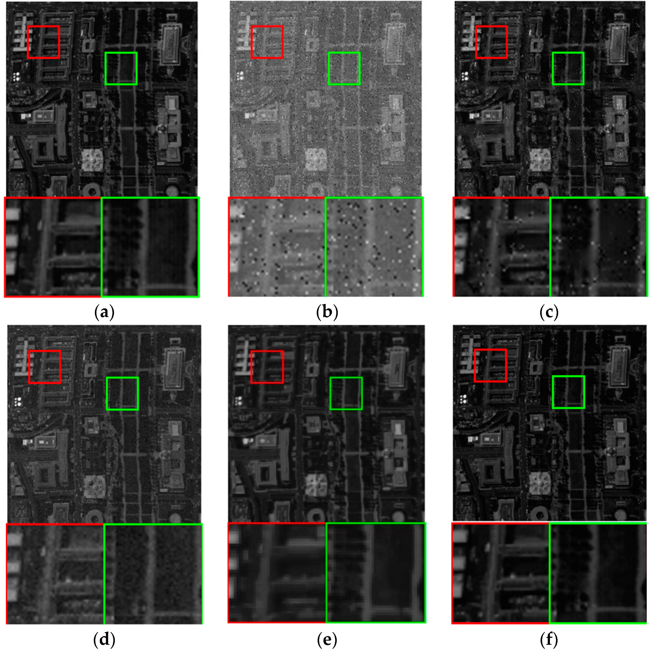
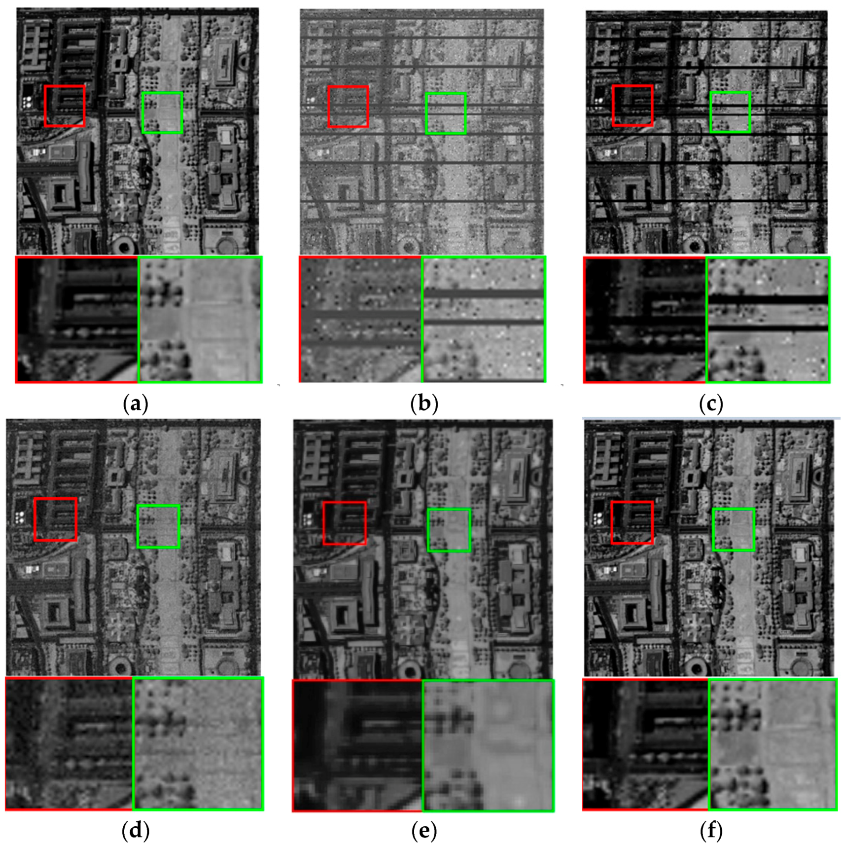
5.2. Performance Evaluation on Simulated Noisy Dataset

When we apply HSI restoration methods on real noisy data, we can only evaluate the performance qualitatively since the noise-free images are always absent in reality, i.e., we evaluate the restoration results by the visual effect.
To obtain both the quantitative and qualitative results, we use the simulate dataset Washington DC Mall as the simulated noise-free image in this study as [11] does. For evaluation purpose, three kinds of common noise are added into this dataset. First, zero-mean Gaussian noise is added into all bands of HSI. Considering the intensity of noise is varied for different bands, we add different bands with different noise intensities. The SNR of the resulted band is ranging from 10db and 20db. Second, we added into HSI uniform noise. Third, we add dead lines, whose width varied from two to three lines, into the bands of 70th to 73rd. For fair comparison, before adding noise into the original HSI, we normalize the gray values of each band between (0, 1)first. Then, we add noise into the normalized image. Finally, the gray values of the denoised image are stretched to the level of original HSI.
Figure 3 and Figure 4 illustrate the experimental results on bands 2 and 100, where two areas of interest are zoomed for a detailed comparison. Those two bands are influenced by Gaussian noise as well as uniform noise. Original clean/noise-free band and the noisy band are shown in (a) and (b). The restoration results via VBM3D, Godec, SLrank, and low-rank methods are given in (c)–(f). By comparing the visual results, it can be seen that the proposed low-rank method has best restoration result among those four methods. The results of Godec based and SLrank based method are oversmoothed and some noise still exists in the denoised image by VBM3D method. This demonstrates that the proposed method functions well for the noisy image. For SLrank based method, its denoising performance is inferior to the proposed method. The reason is given as follows. SLrank based method pays attention on how to accurately recovery image from Gaussian noise or sparse noise polluted images, while the proposed method focuses on a totally new perspective (i.e., how to deal with more kinds of noise) of HSI denoising, which is seldom considered but different with the conditions that SLrank obeys.
Figure 5 and Figure 6 illustrate the restoration results of incomplete bands 70 and 72, which is influenced by uniform noise, Gaussian noise, and dead pixels. The restoration results via VBM3D, Godec, SLrank, and low-rank method are given in (c)–(f). In these figures, two areas of interest are zoomed for a detailed comparison. From the visual results of different methods, it can be seen the results on those two noisy incomplete bands are similar to those in Figure 3 and Figure 4. Noise still obviously exists in the results of VBM3D method. Though Godec based method has comparable restoration results with the proposed low-rank method, some band (band 70) is oversmoothed. Since low-rank matrix analysis is capable of handling the missing data, it can be seen that Godec based, SLrank based, and the proposed low-rank methods simultaneously fill the missing values as well as remove the noise. On the contrary, the dead lines still exist for VBM3D based methods.
Table 1 and Figure 7 give the PSNR and SSIM values. Those values are calculated with all original clean image band and the noisy image band. Figure 7 illustrates the PSNR and SSIM values varied with different bands for different restoration methods, where the vertical axis denotes the PSNR/SSIM values and the horizontal axis denote the band number. In Figure 7, the curves colored with red, blue, green, and black represent the results of VBM3D, Godec, SLrank, and the proposed low-rank, respectively. It can be seen from Figure 7 that the proposed low-rank method has highest PSNR and SSIM value among all competing methods in most bands. The average PSNR and SSIM for all bands are given in Table 1, from which we can see the proposed method obtains better PSNR/SSIM compared with any other competing methods.

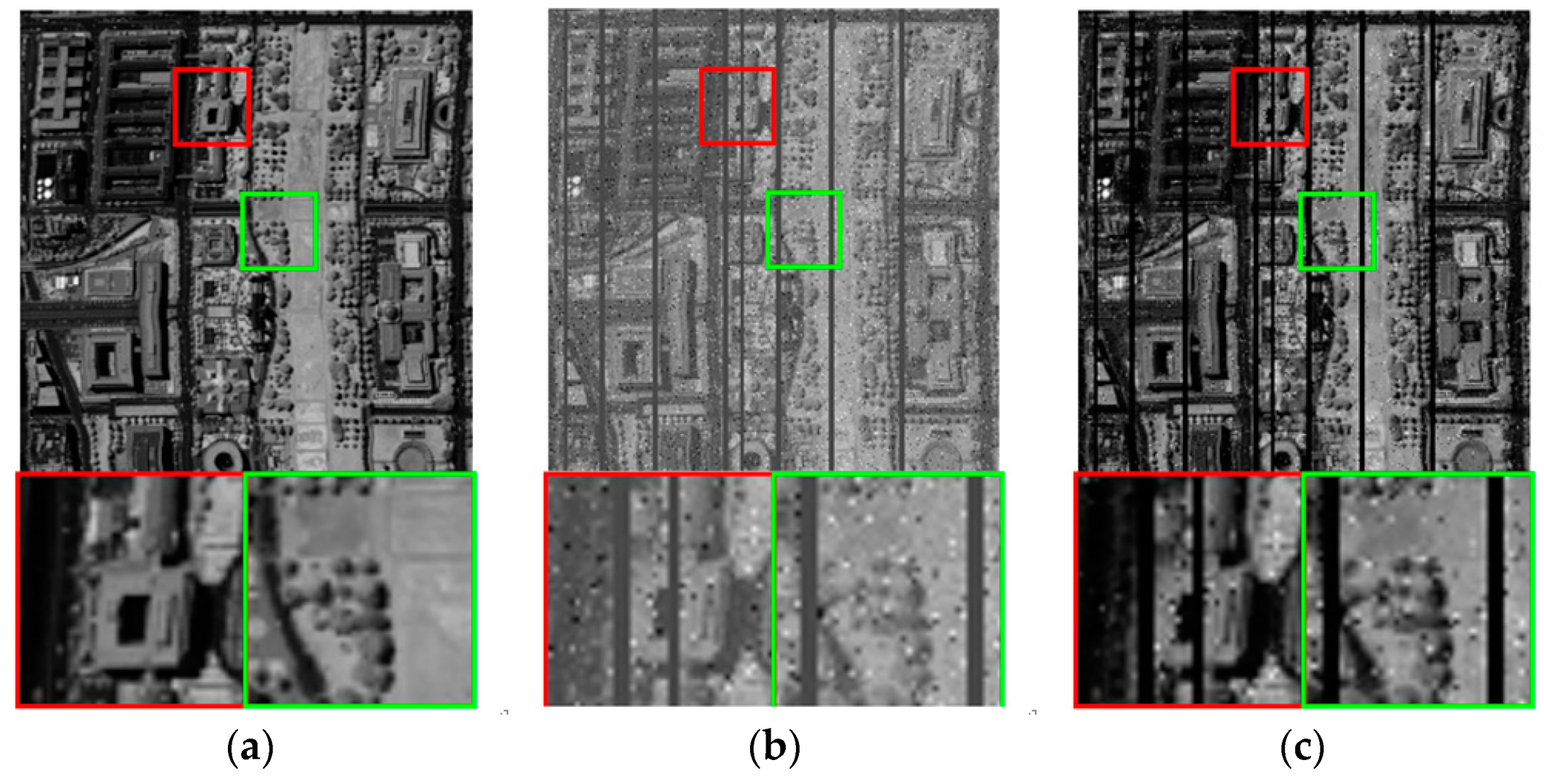
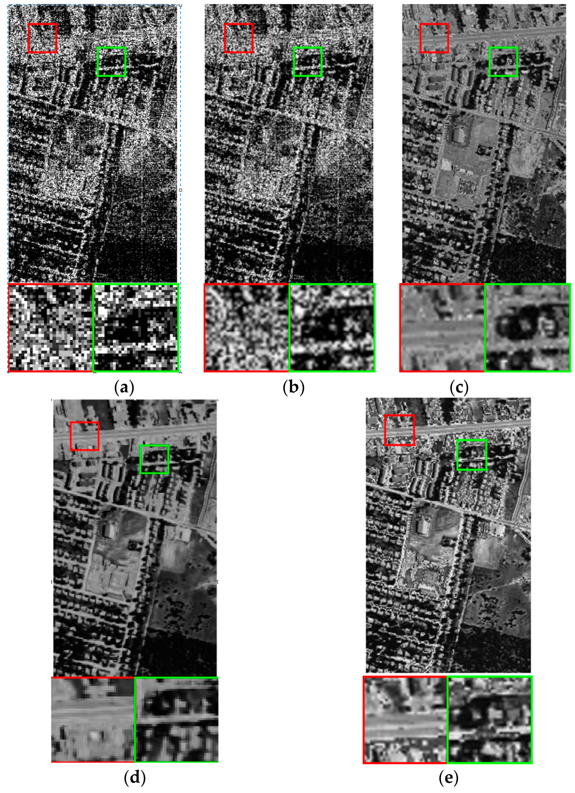
5.3. Evaluation on Real Dataset

We further verify the proposed method on real data. Specifically, we use terrain and urban datasets in the experiments, which can be downloaded from http://www.tec.army.mil/hypercube.
We restore terrain data on all bands with VBM3D, Godec, SLrank, and the proposed low-rank based method. Figure 8 and Figure 9 illustrate the experimental results on bands 1 and 4, where two areas of interest are zoomed. These bands are influenced by Gaussian noise, stripes and dead lines. The real image band is given in (a). The restoration results of VBM3D, Godec, SLrank, and the proposed method are illustrated in (b)–(e). It can be seen that the proposed low-rank method has better performance compared with other competing methods. The stripes and dead lines are well addressed and the details of HSI are well preserved. The dead lines and stripes still remains for VBM3D based method.

6. Discussion

In this paper, an HSI-oriented low-rank denoising method is proposed. According to the experimental results, we can see that:
(1) Low-rank based methods including the proposed, Godec based and SLrank based ones can function better compared with VBM3D based method, especially when confronting with missing values (e.g., dead lines or dead pixels, see from Figure 5 to Figure 6 and Figure 8, Figure 9, Figure 10 and Figure 11). This phenomenon implies that low-rank property is a powerful constraint for HSI restoration. In addition, the result is consistent with the fact that clean/noise-free HSI is a low-rank matrix but the noisy and incomplete HSI is not, thus low-rank property can be used to remove the noise as well as fill in the missing values.
(2) Compared with Godec based method which uses a sparsity item and a Gaussian item to represent noise, mixture of Gaussian distribution introduced in the proposed method is more powerful to represent complex noise since it models each pixel independently. Thus, it guarantees the proposed method is more suitable for HSI restoration (e.g., noise varies across band) and obtains better restoration performance, which can be seen from Figure 3, Figure 4, Figure 5, Figure 6, Figure 7, Figure 8, Figure 9, Figure 10 and Figure 11 and Table 1.
(3) Considering the clean image can be decomposed into the multiplication of two matrices which has lower dimensionality than the original clean image, an endmember determination method is used to automatically determine the rank. It can facilitate the parameter initialization of the low-rank based method, whereas Godec based and SLrank methods need to assign the rank number manually.

7. Conclusions

We propose an HSI-oriented low-rank denoising method in this paper. Considering the clean/noisy-free HSI has a low-rank property and HSI is degraded by multiple kinds of noise, HSI restoration is modeled as a low-rank matrix analysis problem. Specifically, we use the mixture of Gaussian to represent multiple kinds of noise and treat clean HSI as a low-rank matrix. A Bayesian low-rank matrix recovery method is then introduced to infer the low-rank denoised HSI from multi-factor affected incomplete HSI. Considering endmember is an important clue to determine the rank number, a geometry-based endmember determination method is further used to initialize the rank number. The proposed method can address complex noise well and restore the missing data effectively. Experimental results verify the superiority of the proposed method on both simulated and real data.

Author Contributions

W.W. and C.T. designed the algorithm and wrote the manuscript together, W.W. and J.N. conduct the experiment.

Funding

This work is supported by the National Natural Science Foundation of China (no. 61671385, no. 61571354).

Conflicts of Interest

The authors declare no conflict of interest.

References

  1. Ghamisi, P.; Yokoya, N.; Li, J.; Li, W.; Liu, S.; Plaza, J.; Rasti, B.; Plaza, A. Advances in Hyperspectral Image and Signal Processing: A Comprehensive Overview of the State of the Art. IEEE Geosci. Remote Sens. Mag. 2018, 5, 34–78. [Google Scholar] [CrossRef]
  2. Peng, J.; Sun, W.; Du, Q. Self-paced joint sparse representation for the classification of hyperspectral images. IEEE Trans. Geosci. Remote Sens. 2019, 57, 1183–1194. [Google Scholar] [CrossRef]
  3. Bioucas-Dias, J.M.; Plaza, A.; Camps-Valls, G.; Scheunders, P.; Nasabadi, N.; Chanussot, J. Hyperspectral remote sensing data analysis and future challenges. IEEE Geosci. Remote Sens. Mag. 2013, 1, 6–36. [Google Scholar] [CrossRef]
  4. Sun, W.; Du, Q. Graph-regularized fast and robust principal component analysis for hyperspectral band selection. IEEE Trans. Geosci. Remote Sens. 2018, 56, 3185–3195. [Google Scholar] [CrossRef]
  5. Lara, M.Á.; Diezma, B.; Lleó, L.; Roger, J.M.; Garrido, Y.; Gil, M.I.; Ruiz-Altisent, M. Hyperspectral Imaging to Evaluate the Effect of Irrigation Water Salinity in Lettuce. Appl. Sci. 2016, 6, 412. [Google Scholar] [CrossRef]
  6. Sun, W.; Ma, J.; Yang, G.; Du, B.; Zhang, L. A Poisson nonnegative matrix factorization method with parameter subspace clustering constraint for endmember extraction in hyperspectral imagery. ISPRS J. Photogramm. Remote Sens. 2017, 128, 27–39. [Google Scholar] [CrossRef]
  7. Djokam, M.; Sandasi, M.; Chen, W.; Viljoen, A.; Vermaak, I. Hyperspectral Imaging as a Rapid Quality Control Method for Herbal Tea Blends. Appl. Sci. 2017, 7, 268. [Google Scholar] [CrossRef]
  8. Rizkinia, M.; Baba, T.; Shirai, K.; Okuda, M. Local spectral component decomposition for multi-channel image denoising. IEEE Trans. Image Process. 2016, 25, 3208–3218. [Google Scholar] [CrossRef]
  9. Dhuppe, A.; Gaikwad, S.P. Denoising Of Hyperspectral Image. Int. J. Eng. Res. Appl. 2014, 4, 1–10. [Google Scholar]
  10. Wei, W.; Zhang, L.; Tian, C.; Zhang, Y.; Plaza, A. Structured Sparse Coding based Hyperspectral Imagery Denoising with Intra-cluster Filtering. IEEE Trans. Geosci. Remote Sens. 2017, 55, 6860–6876. [Google Scholar] [CrossRef]
  11. Zhang, H.; He, W.; Zhang, L.; Shen, H.; Yuan, Q. Hyperspectral image restoration using low-rank matrix recovery. IEEE Trans. Geosci. Remote Sens. 2014, 52, 4729–4743. [Google Scholar] [CrossRef]
  12. Sun, W.; Yang, G.; Wu, K.; Li, W.; Zhang, D. Pure endmember extraction using robust kernel archetypoid analysis for hyperspectral imagery. ISPRS J. Photogramm. Remote Sens. 2017, 131, 147–159. [Google Scholar] [CrossRef]
  13. Acito, N.; Diani, M.; Corsini, G. Signal-dependent noise modeling and model parameter estimation in hyperspectral images. IEEE Trans. Geosci. Remote Sens. 2011, 48, 2957–2971. [Google Scholar] [CrossRef]
  14. Acito, N.; Diani, M.; Corsini, G. Hyperspectral signal subspace identification in the presence of rare vectors and signal-dependence noise. IEEE Trans. Geosci. Remote Sens. 2013, 51, 283–299. [Google Scholar] [CrossRef]
  15. Caselles, V. Total Variation Based Image Denoising and Restoration. In Proceedings of the International Congress of Mathematicians, Madrid, Spain, 22–30 August 2006. [Google Scholar]
  16. Yu, H.; Zhao, L.; Wang, H. Image denoising using trivariate shrinkage filter in the wavelet domain and joint bilateral filter in the spatial domain. IEEE Trans. Image Process. 2009, 18, 2364–2369. [Google Scholar] [PubMed]
  17. Donoho, D.L.; Johnstone, I.M. Adapting to unknown smoothness via wavelet shrinkage. J. Am. Stat. Assoc. 1995, 90, 1200–1224. [Google Scholar] [CrossRef]
  18. Zelinski, A.C.; Goyal, V.K. Denoising Hyperspectral Imagery and Recovering Junk Bands Using Wavelets and Sparse Approximation. In Proceedings of the International Conference on Geoscience and Remote Sensing Symposium, Denver, CO, USA, 31 July–4 August 2006. [Google Scholar]
  19. Rasti, B.; Sveinsson, J.R.; Ulfarsson, M.O.; Benediktsson, J.A. Hyperspectral Image Denoising Using 3D Wavelets. In Proceedings of the International Conference on Geoscience and Remote Sensing Symposium, Munich, Germany, 22–27 July 2012. [Google Scholar]
  20. Starck, J.-L.; Candes, E.J.; Donoho, D.L. The curvelet transform for image denoising. IEEE Trans. Image Process. 2002, 11, 670–684. [Google Scholar] [CrossRef] [PubMed]
  21. Xu, D.; Sun, L.; Luo, J.; Liu, Z. Analysis and denoising of hyperspectral remote sensing image in the curvelet domain. Math. Probl. Eng. 2013, 2013, 1–11. [Google Scholar] [CrossRef]
  22. Chopra, A.; Lian, H. Total variation, adaptive total variation and nonconvex smoothly clipped absolute deviation penalty for denoising blocky images. Pattern Recognit. 2010, 43, 2609–2619. [Google Scholar] [CrossRef] [Green Version]
  23. Yanovsky, I.; Dragomiretskiy, K. Variational destriping in remote sensing imagery: Total variation with L1 fidelity. Remote Sens. 2018, 10, 300. [Google Scholar] [CrossRef]
  24. Yuan, Q.; Zhang, L.; Shen, H. Hyperspectral image denoising employing a spectral–spatial adaptive total variation model. IEEE Trans. Geosci. Remote Sens. 2012, 50, 3660–3677. [Google Scholar] [CrossRef]
  25. Maboudi, M.; Amini, J.; Hahn, M.; Saati, M. Road Network Extraction from VHR Satellite Images Using Context Aware Object Feature Integration and Tensor Voting. Remote Sens. 2016, 8, 637. [Google Scholar] [CrossRef]
  26. Lin, T.; Bourennane, S. Survey of hyperspectral image denoising methods based on tensor decompositions. EURASIP J. Adv. Signal Process. 2013, 2013, 1–11. [Google Scholar] [CrossRef]
  27. Du, B.; Zhang, M.; Zhang, L.; Hu, R.; Tao, D. PLTD: Patch-Based Low-Rank Tensor Decomposition for Hyperspectral Images. IEEE Trans. Multimed. 2017, 19, 67–79. [Google Scholar] [CrossRef]
  28. Dabov, K.; Foi, A.; Egiazarian, K. Video Denoising by Sparse 3D Transform-Domain Collaborative Filtering. In Proceedings of the European Signal Processing Conference, Poznan, Poland, 3–7 September 2007. [Google Scholar]
  29. Zhao, Y.; Yang, J. Hyperspectral image denoising via sparse representation and low-rank constraint. IEEE Trans. Geosci. Remote Sens. 2015, 53, 296–308. [Google Scholar] [CrossRef]
  30. Danielyan, A.; Katkovnik, V.; Egiazarian, K. BM3D Frames and Variational Image Deblurring. IEEE Trans. Image Process. 2012, 21, 1715–1728. [Google Scholar] [CrossRef] [PubMed]
  31. Zhang, L.; Wei, W.; Tian, C.; Li, F.; Zhang, Y. Exploring structured sparsity by a reweighted laplace prior for hyperspectral compressive sensing. IEEE Trans. Image Process. 2016, 25, 4974–4988. [Google Scholar] [CrossRef]
  32. He, W.; Zhang, H.; Zhang, L.; Shen, H. Total-variation-regularized low-rank matrix factorization for hyperspectral image restoration. IEEE Trans. Geosci. Remote Sens. 2016, 54, 178–188. [Google Scholar] [CrossRef]
  33. Wang, M.; Yu, J.; Xue, J.H.; Sun, W. Denoising of hyperspectral images using group low-rank representation. IEEE J. Sel. Top. Appl. Earth Obs. Remote Sens. 2016, 9, 4420–4427. [Google Scholar] [CrossRef]
  34. Fan, F.; Ma, Y.; Li, C.; Mei, X.; Huang, J.; Ma, J. Hyperspectral image denoising with superpixel segmentation and low-rank representation. Inf. Sci. 2017, 397–398, 48–68. [Google Scholar] [CrossRef]
  35. Wei, W.; Zhang, L.; Jiao, Y.; Tian, C.; Wang, C.; Zhang, Y. Intracluster structured low-rank matrix analysis method for hyperspectral denoising. IEEE Trans. Geosci. Remote Sens. 2019, 57, 866–880. [Google Scholar] [CrossRef]
  36. Li, J.; Bioucas-Dias, J.M.; Plaza, A.; Liu, L. Robust Collaborative Nonnegative Matrix Factorization for Hyperspectral Unmixing. IEEE Trans. Geosci. Remote Sens. 2016, 54, 6076–6090. [Google Scholar] [Green Version]
  37. Bioucas-Dias, J.M.; Nascimento, J. Hyperspectral subspace identification. IEEE Trans. Geosci. Remote Sens. 2008, 46, 2435–2445. [Google Scholar] [CrossRef]
  38. Ambikapathi, A.; Chan, T.H.; Chi, C.Y.; Keizer, K. Hyperspectral Data Geometry-Based Estimation of Number of Endmembers Using p-Norm-Based Pure Pixel Identification Algorithm. IEEE Trans. Geosci. Remote Sens. 2012, 51, 2753–2769. [Google Scholar] [CrossRef]
  39. Candes, E.J.; Li, X.; Ma, Y.; Wright, J. Robust principal component analysis? J. ACM 2011, 58, 1–39. [Google Scholar] [CrossRef]
  40. Wright, J.; Ganesh, A.; Rao, S.; Peng, Y.; Ma, Y. Robust Principal Component Analysis: Exact Recovery of Corrupted low-Rank Matrices Via Convex Optimization. In Proceedings of the Neural Information Processing Systems, Vancouver, BC, Canada, 7–10 December 2009. [Google Scholar]
  41. Zhou, T.; Tao, D. Godec: Randomized Low-Rank & Sparse Matrix Decomposition in Noisy Case. In Proceedings of the International Conference on Machine Learning, Bellevue, Washington, DC, USA, 28 June–2 July 2011. [Google Scholar]
  42. Zhao, Q.; Meng, D.; Xu, Z.; Zuo, W.; Zhang, L. Robust Principal Component Analysis with Complex Noise. In Proceedings of the International Conference on Machine Learning, Beijing, China, 22–24 June 2014. [Google Scholar]
  43. Babacan, S.D.; Luessi, M.; Molina, R.; Katsaggelos, A.K. Sparse bayesian methods for low-rank matrix estimation. IEEE Trans. Signal Process. 2012, 60, 3964–3977. [Google Scholar] [CrossRef]
Figure 1. Illustration of the hyperspectral linear mixed model.
Applsci 09 02529 g001
Figure 2. Framework of the proposed method.
Applsci 09 02529 g002
Figure 3. Visual comparison on band 2 of Washington dataset: (a) Clean/noise-free image band, (b) Noisy band, (c) Restoration result from VBM3D, (d) Restoration result from Godec, (e) Restoration result from SLrank, (f) Restoration result from the proposed method.
Applsci 09 02529 g003
Figure 4. Visual comparison on band 100 of Washington dataset: (a) Clean/noise-free image band, (b) Noisy band, (c) Restoration result from VBM3D, (d) Restoration result from Godec, (e) Restoration result from SLrank, (f) Restoration result from the proposed method.
Applsci 09 02529 g004
Figure 5. Visual comparison on band 70 of Washington dataset: (a) Clean/noise-free image band, (b) Noisy band, (c) Restoration result from VBM3D, (d) Restoration result from Godec, (e) Restoration result from SLrank, (f) Restoration result from the proposed method.
Applsci 09 02529 g005
Figure 6. Visual comparison on band 72 of Washington dataset: (a) Clean/noise-free image band, (b) Noisy band, (c) Restoration result from VBM3D, (d) Restoration result from Godec, (e) Restoration result from SLrank, (f) Restoration result from the proposed method.
Applsci 09 02529 g006aApplsci 09 02529 g006b
Figure 7. PSNR and SSIM values varied with different bands for different restoration methods.
Applsci 09 02529 g007
Figure 8. Visual results on band 1 of terrain dataset: (a) Captured actual band, (b) Restoration results of VBM3D based method, (c) Restoration results of Godec based method, (d) Restoration results of SLrank based method, (e) Restoration results of the proposed method.
Applsci 09 02529 g008
Figure 9. Visual results on band 4 of terrain dataset: (a) Captured actual band, (b) Restoration results of VBM3D based method, (c) Restoration results of Godec based method, (d) Restoration results of SLrank based method, (e) Restoration results of the proposed method.
Applsci 09 02529 g009
Figure 10. Visual results on band 2 of urban dataset: (a) Captured actual band, (b) Restoration results of VBM3D based method, (c) Restoration results of Godec based method, (d) Restoration results of SLrank based method, (e) Restoration results of the proposed method.
Applsci 09 02529 g010
Figure 11. Visual results on band 188 of urban dataset: (a) Captured actual band, (b) Restoration results of VBM3D based method, (c) Restoration results of Godec based method, (d) Restoration results of SLrank based method, (e) Restoration results of the proposed method.
Applsci 09 02529 g011
Table 1. Average peak signal-to-noise ratio (PSNR) and structure similarity (SSIM)for different restoration methods.
VBM3DGodecSLrankLow-Rank
PSNR13.5711.8713.1216.13
SSIM0.770.790.830.95

