Abstract
The quality of positioning services based on Global Navigation Satellite Systems (GNSS) is improving at a fast pace, driven by the strict requirements of a plethora of new applications on accuracy, precision and reliability of the services. Nevertheless, ionospheric errors still bound the achievable performance and better mitigation techniques must be devised. In particular, the harmful effect due to non-uniform distribution of the electron density that causes amplitude and phase variation of the GNSS signal, usually named as scintillation effects. For many high-accuracy applications, this is a threat to accuracy and reliability, and the presence of scintillation effect needs to be constantly monitored. To this purpose, traditional receivers employ closed-loop tracking architectures. In this paper, we investigate an alternative architecture and a related metric based on the statistical processing of the received signal, after a code-wipe off and a noise reduction phase. The new metric is based on the analysis of the statistical features of the conditioned signal, and it brings the same information of the index, normally estimated by means of closed-loop receivers. This new metric can be obtained at a higher rate as well as in the case of strong scintillations when a closed-loop receiver would fail the tracking of the GNSS signals.
1. Introduction
The modernisation of the Global Navigation Satellite System (GNSS) and the constant improvement of their performance is driving the design of a plethora of applications with strict requirements on accuracy, precision and reliability of the estimated position [1]. Despite the impressive improvement of the quality of the broadcast signals and new processing techniques, the propagation of the signal through the ionosphere is still one of the limiting factors for precise positioning. In fact, it is well known that the GNSS signals while travelling through the upper layers of the athmosphere are affected in terms of delay, amplitude and phase, which turn out to be different with respect to the assumed propagation in free-space. Compensation of the ionospheric delay is applied by now in any GNSS receiver, either using models or external assistance for single frequency receivers, and it can be compensated by means of the iono-free combination of the measured pseudoranges in multi-frequency receivers [2]. However, due to the presence of a non-uniform distribution of the electron density in some layers of the ionosphere, electromagnetic signals are scattered in random directions, thus reaching the Earth through multiple paths. Signals on each path add in a phase-wise sense and interfere with each other, so that the received signal is then affected by deep amplitude fading and phase fluctuations.
GNSS signals are indeed affected by scintillation effects, and their quality at the receiver might be strongly degraded. While moderate scintillations only increase noise in code and phase measurements, strong scintillation events severely disrupt the capabilities of GNSS receivers. Amplitude fading and rapid phase changes impact the receivers’ tracking loops capabilities to follow the signal dynamics, resulting in cycle slips and Loss-of-Lock (LoL) in the tracking stage of the receiver [3]. Phase range measurements errors can be from 3 to 10 times larger [4], whereas, in the most severe situations, when more than one satellite-receiver link is concerned and the satellite visibility is poor, the receiver might completely fail [5]. At the same time, thanks to their global coverage and continuous availability, GNSS signals provide an excellent means to monitor the activity of the ionosphere. With multiple satellites from multiple constellations, the physical effects can be simultaneously measured through many pierce points. GNSS receivers have then become a convenient, cheap and widespread tool to study such phenomena [6,7].
In this paper, we propose a technique to assess the intensity of scintillation on the signal amplitude, which is an alternative to the classical methods that require a GNSS receiver employing closed-loop architectures. Rather then relying on the traditional commercial receiver architecture, in which only the correlator outputs are available to the end user, this approach fully exploits the flexibility of a receiver architecture entirely designed according to software-radio approach [8]. Samples of the received signal at Radio Frequency (RF) are collected, sampled and digitized, at sampling frequencies of the order of millions of samples per second. Then, the bit-stream is stored on memories and processed by a fully-software GNSS receiver. This approach has gained consensus in recent years also in the space weather community [9,10,11], and it allows for an easier implementation of novel algorithms, specifically tailored to the scintillation monitoring and mitigation [12]. As a consequence, such techniques can be robust by design to the strong scintillations events causing LoLs in classical receivers’ architectures.
The paper is organized as follows: Section 2 will briefly recall the well known parameters used for scintillation detection and classification. Section 3 will discuss the flexibility given by a software-defined-radio approach for the design of novel methods to process the digitized GNSS signal, including the possibility to undertake different approaches for the scintillation monitoring. Section 4 discusses the impact of scintillation on the classical closed-loop architectures. The core of the paper is introduced in Section 5, where an open loop architecture is proposed to implement a robust interference monitoring platform, and in Section 6 new metrics are presented. Finally, Section 7 will present the results obtained processing real data collected during scintillation events.
2. GNSS Scintillation Measurement
As previously recalled, ionospheric scintillations are rapid and hard-to-predict fluctuations of the amplitude and phase of radio signals propagating through the atmosphere. The propagation through ionosphere is one of the main error sources affecting the GNSS signal processing stages of the receiver. In fact, the signal is potentially affected by strong degradation, introducing significant problems in any GNSS application requiring high accuracy, precision, reliability and continuity. On the other hand, scintillation mitigation is still an open issue in most of the commercial devices, mainly due to the inherently random nature of such events, which makes modelling impossible [13]. Scintillations are then, at the moment, one of the main limiting factors for high accuracy applications.
Scintillation events are traditionally characterized by means of two indices evaluated over an 60 s observation interval.
- The amplitude scintillation index, named , estimates the amount of amplitude fluctuations. Such an index is computed as the normalized standard deviation of the detrended Signal Intensity (SI), derived from in-phase (I) and quadrature (Q) prompt correlation outputs, normalized by its mean value.
- The phase scintillation index denoted measuring the impact on the phase of the signal; it is equivalent to the standard deviation of the detrended carrier phase measure.
The majority of the works related to scintillation detection and monitoring are based on the analysis of the value of these two indices, often comparing them with predefined thresholds. However, the estimation of and requires the GNSS receiver to be in lock conditions, i.e., the values of I and Q correlators must be available. In the case of strong scintillation events, receivers designed according to the classical closed-loop architecture might not be robust enough to keep the correct tracking of the signals, incurring in a LoL event. If this happens, the receiver is not able to provide the values needed to characterize the the scintillation event, which is, in a generic way, classified as “strong”. At the same time, the computation of and requires a detrending operation, which envisages the use non-trivial mathematical operations. Although this process has been standardized and is largely used, several authors pointed out that it can introduce artifacts in the signal processing chain falsifying the scintillation estimation [14,15]. This opens the way to the definition of alternative measures of scintillation [14,16,17,18].
Some of these methods start from the observation that, in the presence of scintillations, the statistics of the samples of the amplitudes change over time and it is correlated to the values taken by the index. In statistical terms, according to [4], scintillation-derived amplitude fluctuations follow a Nakagami-m distribution, the shape of which depends on the severity of the fluctuations. This is depicted in Figure 1, where the histograms of the samples for different values are displayed. The method introduced in this paper aims at estimating the statistic of the amplitude samples in the presence of scintillations, building on top of that a new metric for the characterisation of the scintillation event, as will be explained in the following sections.
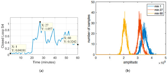
Figure 1.
The distribution of the signal samples varies according to scintillation intensity; (a) values of the amplitude scintillation index over time; (b) histogram of the Signal Intensity (SI) for three different values of amplitude scintillation taken at three different time instants.
3. The Software-Radio Approach for Ionospheric Monitoring
Ionosphere monitoring has traditionally been a prerogative of professional and commercial hardware GNSS receivers. Devices specifically designed for the analysis of ionospheric events are denoted Ionospheric Scintillation Monitoring Receivers (ISMRs). Nevertheless, recent trends in GNSS receivers implementation envisage the use of Software Defined Radio (SDR) technology, as a valuable alternative to commercial GNSS receivers. In its general view, SDR refers to the ensemble of hardware and software technologies and design choices enabling reconfigurable radio communication architectures [19]. According to this paradigm, all of the signal processing stages of the receiver chain are implemented as software routines. Contrarily to hardware GNSS receivers, where only post-processed data are available, software-defined receivers allow users to access any intermediate and low-level signal processing stage, and, in turn, a wider, potentially unlimited, set of observables [8]. In addition, the software implementation grants a complete control of the receiver architecture, in terms of configuration and of implementation of novel algorithms, including ionospheric monitoring [20].
GNSS SDR receiver architecture is commonly divided into two blocks, as reported in Figure 2.
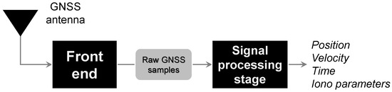
Figure 2.
Generic architecture of a Software Defined Radio (SDR) satellite navigation receiver.
- The data grabber, composed by an antenna and an RF front-end; the GNSS signal is pre-conditioned, down-converted at Intermediate Frequency (IF), sampled and digitized by an Analog-to-Digital Converter (ADC); then, raw IF samples are stored on memories.
- The signal processing stage, fully implemented in software, where the stored samples are processed, either in real-time or in post-processing.
Examples of SDR implementations for scintillation monitoring are given for instance in [9,10,11,21]. The flexibility granted by this approach eases the implementation of monitoring stations in harsh environments [22,23], and also the design of new signal processing methods for GNSS signal monitoring [15,24,25].
4. Impact of Strong Scintillations on GNSS Receivers
One of the consequences of scintillation is LoL of the tracking stages of the receiver, affecting the quality of navigation solution and also making impossible the calculation of the scintillation activity through the classical indices. In case of LoL, the computation of indices using tracking loop outputs is not reliable, thus leading to false alarms and missed detections of the monitoring unit.
An example of LoL due to strong amplitude scintillation in closed loops is reported in Figure 3. From top to bottom, the values of the I and Q prompt correlators, the estimate of the , the values of the Phase Lock Loop (PLL) discriminator output, the estimate of the Doppler frequency and the estimated value are reported. Figure 3a reports the tracking results obtained running a classical second order tracking loop. After about five minutes, the fading induced by amplitude scintillation is so strong that the PLL loses the lock on the signal. As a consequence, the values provided by the scintillation monitoring engine, and computed upon the values of the I and Q correlators, cannot be trusted. As a benchmark, the results obtained running an experimental third order loop, especially configured in terms of bandwidth and loop parameters to be able to track such extreme fading situations, are reported in Figure 3b. The third order loop is able to keep the lock on the signal, even though the quality of the measurements is low. In this case, the estimate of the can then be considered valid. It is worth noting that, for the first five minutes, the two architectures provide the same value of the index, while, after the loss of lock, the values provided by the 2nd order PLL are false, and, in particular, they underestimate the intensity of the scintillation event.
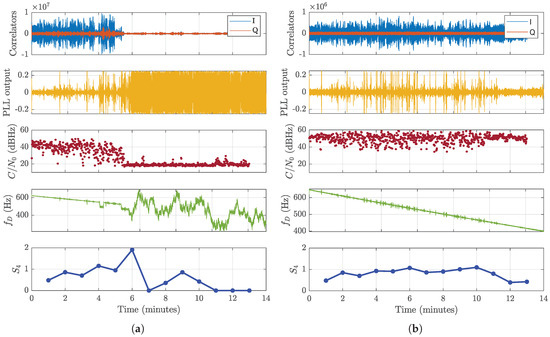
Figure 3.
Example of Loss of Lock (LoL) under strong amplitude scintillation in a closed loop receiver; (a) second order Phase Lock Loop (PLL) implementation; (b) experimental third order PLL.
In general, under significant scintillation events, cycle slips, degradation of and corruption of data bits affects the quality of the estimated position (since some satellites might have to be excluded from the solution). In addition, the estimations of values for the affected channels are wrong, as shown in Figure 3a.
Various techniques are proposed in the literature to reduce the probability of a LoL in the presence of scintillation. The straightforward solution is indeed to exploit a third order PLL [26,27], as shown by the previous example, but also advanced receiver architectures have been proposed, [12]. However, the only solution able to completely overcome the problem of LoLs is to abandon the closed loop implementation in favour of an open loop architecture [18,28]. It is, of course, well known that closed loop solutions are optimal in terms of limiting the jitter on the code and phase estimations, but they show limitations for the specific use in scintillation monitoring receivers in the presence of strong events.
In the following sections, an open loop architecture will be exploited to extract from the incoming signal the information related to the amplitude scintillation intensity, defining a metric alternative to the parameter. This architecture has been firstly presented in a previous paper of the authors [18], but has been refined and extended in the present work. A similar approach has been proposed in other works (such as [29,30]); however, the architecture proposed in this study overcomes several limitations, among which the need of a fine time assistance.
5. Open Loop Processing Architecture
The key concept of GNSS open loop processing, which is depicted in Figure 4, is that, as long as the receiver is static, its reference position and time are known, and a network connection providing A-GNSS messages is available; some of the components of the signal can be considered as known, or properly predicted. The knowledge of such components can then be exploited to remove them from the incoming signal, leaving only the random contributions that are due to the thermal noise and other disturbances, among which are the scintillation effects. Scintillation contributions can then be separated from the GNSS signal, which can be considered a sort of deterministic, periodic contribution in the overall received signal.
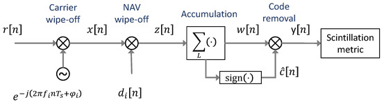
Figure 4.
Block diagram of the assisted open loop architecture used to perform the analysis.
Let
be the discrete version of the received signal at the output of the analog-to-digital converter of the front-end which operates at a sampling frequency on the GNSS signal at IF. is the number of satellites in view, each of one contributing to the overall received signal; the pedix i refers to the i-th satellite; is the navigation message; is the code delay; is the spreading code; is the carrier frequency, which includes the nominal intermediate frequency and the Doppler frequency shift ; is a generic phase contribution; and is thermal noise.
The architecture does not include either a PLL or a Frequency Lock Loop (FLL) demodulating the signal to baseband by removing the residual carrier at frequency . The residual carrier is wiped-off using the Doppler information from assistance. Such assistance information is a good estimate of , but it does not include the spurious effect that can be due to the instability of the front-end clock. For such a reason, a good quality clock with negligible frequency drift has to be used to drive both the sampling stage and the frequency references in the front-end. The effect of the non-perfect carrier removal and the issues related to the Doppler shift estimation will be discussed in Section 5.2. Let us assume, for sake of simplicity at this stage, that the estimation of the Doppler frequency is perfect and then that the carrier the wipe-off demodulates the signal to baseband. The mixing generates images of the spectrum at a harmonics frequency, which are removed by the accumulation process, acts as a low pass filter. The signal , after carrier wipe-off, and assuming perfect time synchronization and ideal filtering, can then be expressed as:
and is, in general, a complex number, due to the multiplication times a complex exponential.
As a following step, if a data channel is considered, the navigation message has to be removed, (e.g., exploiting assistance message and the reference time at the receiver). Small errors in this process can be tolerated, as they introduce negligible losses, as it will be shown later. The signal , after navigation message wipe-off, and assuming perfect time synchronization, can then be expressed as:
Because of the presence of thermal noise , the Pseudo Random Noise (PRN) spreading code is not visible and therefore it is not yet possible to estimate and remove it. In principle, the PRN code could be removed by a wipe-off operation, as in a pure open loop receiver, but this would require sub chip-level time synchronization and fine assistance [31,32]. This condition is difficult to be satisfied only exploiting proper A-GNSS information and good knowledge of the position of the receiver. Therefore, a different strategy for code removal has to be identified, based on a blind self-estimation of the code. Since thermal noise can be modeled as a zero mean Gaussian random variable, an accumulation process can increase the SNR (Signal-to-Noise Ratio) of the signal up to the point in which the code chips emerge from the noise floor. The digital signal after carrier and data wipe-off, , is divided in chunks of length , where is the spreading code periodicity, as, for example, 1 ms for the GPS C/A signal. Supposing a period is composed of N samples, L periods are coherently summed together, obtaining the signal of length N
as depicted in Figure 5.
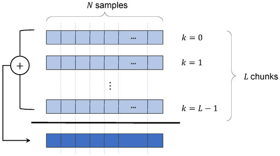
Figure 5.
Accumulation of L chunks of N samples.
The scope of this coherent accumulation is the estimation of the GNSS spreading code, and this technique has been widely used in the past for the blind identification of the codes transmitted by new GNSS satellites [33] or to detect anomalies and evil waveforms [34,35]. The estimated binary GNSS code can be extracted by means of the sign operator:
The spreading code is then wiped-off from the GNSS signal, by multiplying the binary sequence times the signal at output of the accumulation, , thus obtaining a complex signal affected only by a residual noise component and by scintillation:
The digital signal is eventually fed to the scintillation metric block.
The code retrieval process is depicted in Figure 6: few chips of the the signal after accumulation, , are depicted in blue, while the estimated binary spreading code is depicted in red. On the reconstructed code , some residual distortion can be noted due to any other un-modeled effect that cannot be averaged to zero by the accumulation process, and, as well, due to some residual noise contribution.
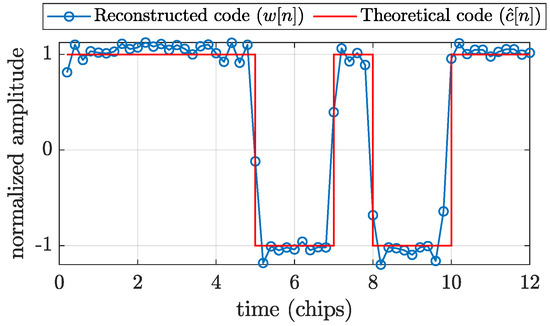
Figure 6.
Reconstructed code with transition samples vs. theoretical code.
5.1. Trade-Off between Noise Average and Observation Rate
The signal will be processed by the scintillation analysis block that will perform a statistical analysis of the samples. For this reason, the noise contribution still affecting the signal after the accumulation has to be sufficiently small, so that it does not mask or bias the results.
Given a fixed sampling frequency , increasing L, the noise contribution tends to be averaged out, but this would require many segments of received signal, i.e., a large observation window . Due to the non-stationarity of the scintillation process, the statistical distribution of the signal amplitude changes over time. This limits the increasing of L that, if chosen to be too large, would not catch the significant changes on the statistic distribution since they would be all included in the same observation window. The parameter L must trade off this resolution in time of the analysis with the capability of reducing the noise effect.
As a trade-off between the noise averaging and the resolution in time for the GPS C/A code, , corresponding to five seconds of the received signal, was heuristically chosen. Therefore, from now on, signals obtained accumulating over 5000 periods of ms of signal, are adopted for scintillation analysis of the GPS C/A code.
5.2. Transition Samples
In order to be able to coherently accumulate the code periods, the carrier removal must be very effective. The Doppler frequency shift affecting the signal can indeed be derived from A-GNSS information, combining the information on the satellites’ position and velocities and the known user position. Therefore, the residual carrier can be ideally wiped-off. Similarly, the navigation message can be perfectly removed, by exploiting A-GNSS aiding. However, the Doppler effect does not only change the carrier frequency, but also the code rate, causing it to stretch and compress. Supposing to be the nominal chip rate, the transmission frequency, it can be found that the actual chip rate at time t, is:
where is Doppler frequency shift on the carrier at time t.
Given a fixed sampling frequency , the time varying code rate induces a change in the number of samples per code chip from period to period. Furthermore, and are not likely to be multiples of each other. The result is that the same chip, in subsequent PRN code periods, might not be represented by the same number of samples. In other words, subsequent sampled chips might not be perfectly aligned, thus threatening the effects of the coherent accumulation of the code periods.
Ideally, after the accumulation process, an exact representation of the spreading code would be obtained, as depicted by perfect rectangular wave plotted in red in Figure 6. However, in a realistic situation, as shown in blue in Figure 6, the non-perfect alignment of the samples leads to “transition samples” at the boundaries of the chips that are wrongly reconstructed by the quantization performed by the sign function.
Transition samples cannot be avoided, unless a very low value of L is used, which could, in turn, prevent a correct extraction of the code from the noise. The effect of transition samples over the overall statistic of samples is depicted in Figure 7, where histograms of with and without transition samples are reported. Figure 7a clearly shows a tail in the distribution towards zero, due to the transition samples.
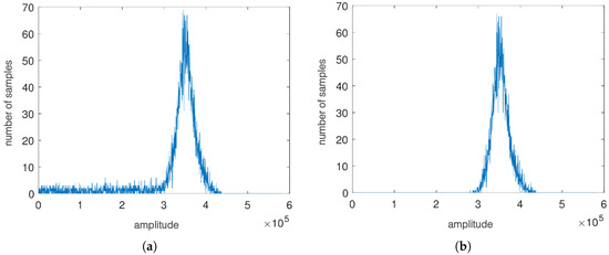
Figure 7.
Distribution of the samples after accumulation, ; (a) in presence of transition samples; (b) in absence of transition samples.
If transition samples are not removed from , a residual modulation remains in after the code wipe-off. Their presence can indeed alter the statistic analysis performed to extract scintillation metrics. For this reason, a simple algorithm to discard transition samples has been implemented, discarding both the sample before and after a sign transition. This strategy avoids the definition of thresholds of a multilevel non-uniform quantizer for the removal of the transition samples, which could introduce further artifacts in the signal processing chain.
6. Scintillation Statistical Analysis
The scintillation analysis is performed through a goodness of fit process taking into account the statistical distribution of the samples in the cases with and without scintillation effects.
A scintillation-free reference curve is created best-fitting a Gaussian curve to the distribution of the samples in absence of scintillation. corresponds to the distribution of the samples for the time interval under test. If fit is accurate, is a good approximation, then there is no scintillation, and, vice versa, scintillation is declared present.
The model curve for estimating is
in which a, b, c are estimated on the basis of an iterative method that minimizes the sum S of squared residuals
where
Figure 8 reports an example, depicting the reference curve and the histogram of a set of samples that includes both scintallated and non-scintillated samples. As it can be noted, the Gaussian fitting is able to match only the non-scintillated part of the histogram, while in the presence of scintillation, the samples are distributed according to the typical Nakagami-m probability density function, thus deviating from obtained in case of no scintillation.
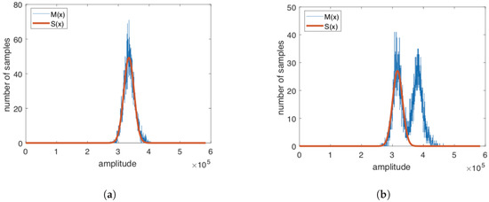
Figure 8.
Change of the distribution in the presence of scintillations. (a) best fitting Gaussian distribution in absence of scintillations; (b) histogram of the samples for a time window including both samples affected by scintillations and not affected. A Gaussian best fitting would be able to match only the “non-scintillated” part of the histogram.
In statistics, to evaluate the goodness of fit, the parameter
is used, where is the mean of , and are the values of the best-fitting Gaussian distribution for the non-scintillated case. can vary in the interval . The greater , the better the fitting and vice versa. A measure of diversity can then be defined through a novel parameter denoted and defined as
7. Validation and Use of the Open-Loop Metrics
In this section, in order to validate the definition of the the new metrics and demonstrate their use, real datasets collected in low-latitude regions are used. A first dataset is derived from the data collection campaign collected in the frame of the MImOSA project [36] by means of a GNSS SDR data acquisition system [8]. Data are related to GPS L1 C/A signal collected along equatorial regions at −22.120045° N, −51.408671° E on 25 March 2015. The signal was sampled at 5 Msamples/s, with a resolution of 16 bits, and demodulated at baseband. To measure the effects of scintillations, the and parameters are employed and compared. The has been computed by means of a software routine processing the I and Q correlator outputs provided by the closed loop tracking of a GNSS software receiver, and following the methodology explained in Section 3. has been derived following computations of Section 6. In such a data collection, several satellite-receiver links are affected by scintillations. Figure 9 plots the and obtained for PRN1 and PRN3. In particular, values are shown in blue and with a rate of Hz, whereas, in red, R4 values are reported with a rate of Hz.
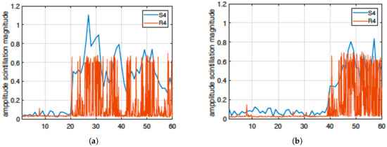
Figure 9.
Comparison of and parameters: (a) GPS PRN 1, (b) GPS PRN 3.
It can be noted that and are somehow correlated. However, is obtained at a higher rate than , and, being based on the open-loop architecture, it does not require the tracking to be locked, i.e., it can be obtained also in case of strong scintillation events that threaten the correct operation of a GNSS receiver, as detailed in Section 7.1.
In order to demonstrate that is actually carrying the same information of , a filtering operation is applied to values to resemble values. A moving average window of width and with amplitude is used. Parameters and were obtained minimizing the root mean square error between the two curves over a large dataset of scintillation events representative of all possible dynamics. Similarity between the curves in Figure 10 shows how follows the same trend of the classical index and thus it carries the same kind of information. This comparison validates the definition of as an alternative to that can be obtained at a higher rate. When, in case of strong events, the estimation of is not available or not reliable, can still be calculated and it extrapolates the same kind of information carried by also in these threatening scenarios.
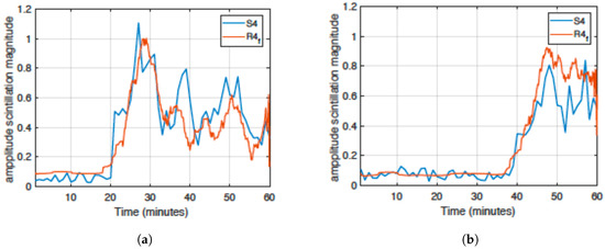
Figure 10.
Comparison of and parameters after filtering: (a) GPS PRN 1, (b) GPS PRN 3.
Furthermore, many recent works on scintillation are questioning the validity of the classical algorithm for estimation, mainly because of the detrending procedures involved, which, if not properly tuned, might mask or falsify scintillation events. A different index, independent from , not requiring detrending operations, and exploiting technological advances such as software defined receivers, might help in this process of redefining the metrics for the characterization of the scintillation events [14,37].
7.1. Case of Loss of Lock
In order to test the goodness of the open loop approach in the presence of a loss of lock, the same case study reported in Section 4 is analyzed. It has to be remarked how , being based on an open loop architecture, is not prone to LoL, and it can work also in case of very strong scintillations. Figure 11 reports the value of the filtered metric, obtained by processing the raw signal samples by means of the open loop receiver. This is compared to the values of the obtained by the second order closed loop receiver, as reported in Figure 3a, where a LoL occurred after about five minutes. In order to benchmark the results, a reference , obtained by a commercial scintillation monitoring receiver, is plotted, corresponding to the estimate obtained running a robust third order loop, as shown in Figure 3b.
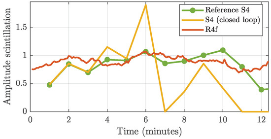
Figure 11.
Comparison of and parameters after filtering, for a LoL case.
As already observed, the estimate from the closed loop cannot be trusted after minute 5, due to the incorrect values of the I and Q correlator outputs. On the contrary, the metric derived from the open loop processing follows the same trend of the reference , thus confirming the validity of the proposed technique in the presence of strong amplitude scintillations inducing losses of lock in traditional receiver architectures.
8. Conclusions
This paper presents a novel method to measure the impact of amplitude ionospheric scintillations of GNSS trans-ionospheric signals, based on statistical considerations on the distribution of the samples at the output and on open loop architecture. Despite being one of the major sources of error affecting high accuracy GNSS applications, ionospheric scintillations are an important tool to study the behavior of this layer of the atmosphere. However, strong events prevent the receiver from correctly tracking the signal, thus producing erroneous scintillation measures. The quality of traditional indices can also be questioned by the detrending operation. To overcome such problems, an alternative measure is derived, exploiting an assisted open loop approach specifically designed for this task in a GNSS software defined radio receiver. The mathematical and technical details of the receiver implementation are given, along with the description of the alternative amplitude scintillation index . The validity of the proposed approach is confirmed by the results obtained processing real GNSS data affected by amplitude scintillations, and by comparing them with the traditional index based on the closed loop approach. In addition, the paper reports the case of strong scintillation that produces a LoL, completely preventing the traditional closed loop to track the signal and to produce a valid measure of ; the proposed technique, instead, shows a valid and reliable amplitude scintillation measure.
References
Author Contributions
Conceptualization, F.D. and N.L.; Methodology, F.D. and N.L.; Software, N.L.; Validation, F.D. and N.L.; Formal Analysis, F.D.; Investigation, F.D. and N.L.; Data Curation, N.L.
Funding
This research received no external funding.
Acknowledgments
The authors would like to thank Ariel Belga Fedeli for the contribution he provided to this work.
Conflicts of Interest
The authors declare no conflict of interest.
References
- Dovis, F.; Margaria, D.; Mulassano, P.; Dominici, F. Overview of Global Positioning Systems. In Handbook of Position Location: Theory, Practice, and Advances, 2nd ed.; Zekavat, R., Buehrer, R.M., Eds.; Wiley-IEEE Press: Hoboken, NJ, USA, 2019; pp. 655–705. [Google Scholar] [CrossRef]
- Kaplan, E.D.; Hegarty, C. Understanding GPS/GNSS: Principles and Applications, 3rd ed.; Artech House: Norwood, MA, USA, 2017. [Google Scholar]
- Lo Presti, L.; Fantino, M.; Pini, M. Digital Signal Processsing for GNSS receivers. In Handbook of Position Location: Theory, Practice, and Advances, 2nd ed.; Zekavat, R., Buehrer, R.M., Eds.; Wiley-IEEE Press: Hoboken, NJ, USA, 2019; pp. 707–761. [Google Scholar] [CrossRef]
- Humphreys, T.E.; Psiaki, M.L.; Hinks, J.C.; O’Hanlon, B.; Kintner, P.M. Simulating Ionosphere-Induced Scintillation for Testing GPS Receiver Phase Tracking Loops. IEEE J. Sel. Top. Signal Process. 2009, 3, 707–715. [Google Scholar] [CrossRef]
- Kintner, P.; Ledvina, B.; De Paula, E. GPS and ionospheric scintillations. Space Weather 2007, 5, 1–23. [Google Scholar] [CrossRef]
- Spogli, L.; Alfonsi, L.; De Franceschi, G.; Romano, V.; Aquino, M.H.O.; Dodson, A. Climatology of GPS ionospheric scintillations over high and mid-latitude European regions. Ann. Geophys. 2009, 27, 3429–3437. [Google Scholar] [CrossRef]
- Povero, G.; Alfonsi, L.; Spogli, L.; Di Mauro, D.; Cesaroni, C.; Dovis, F.; Romero, R.; Abadi, P.; Le Huy, M.; La The, V.; et al. Ionosphere Monitoring in South East Asia in the ERICA Study. Navigation 2017, 64, 273–287. [Google Scholar] [CrossRef]
- Cristodaro, C.; Dovis, F.; Linty, N.; Romero, R. Design of a Configurable Monitoring Station for Scintillations by Means of a GNSS Software Radio Receiver. IEEE Geosci. Remote Sens. Lett. 2018, 15, 325–329. [Google Scholar] [CrossRef]
- Curran, J.T.; Bavaro, M.; Morrison, A.; Fortuny, J. Developing a Multi-Frequency for GNSS-Based Scintillation Monitoring Receiver. In Proceedings of the 27th International Technical Meeting of The Satellite Division of the Institute of Navigation (ION GNSS+ 2014), Tampa, FL, USA, 8–12 September 2014; pp. 1142–1152. [Google Scholar]
- Peng, S.; Morton, Y. A USRP2-based reconfigurable multi- constellation multi-frequency GNSS software receiver front end. GPS Solut. 2013, 17, 89–102. [Google Scholar] [CrossRef]
- Linty, N.; Dovis, F.; Alfonsi, L. Software-defined radio technology for GNSS scintillation analysis: Bring Antarctica to the lab. GPS Solut. 2018, 22, 96. [Google Scholar] [CrossRef]
- Vilà-Valls, J.; Closas, P.; Fernández-Prades, C.; Curran, J.T. On the Mitigation of Ionospheric Scintillation in Advanced GNSS Receivers. IEEE Trans. Aerosp. Electron. Syst. 2018, 54, 1692–1708. [Google Scholar] [CrossRef]
- Van Dierendonck, A.; Klobuchar, J.; Hua, Q. Ionospheric scintillation monitoring using commercial single frequency C/A code receivers. In Proceedings of the 6th International Technical Meeting of the Satellite Division of The Institute of Navigation (ION GPS 1993), Salt Lake City, UT, USA, 22–24 September 1993; Volume 93, pp. 1333–1342. [Google Scholar]
- Mushini, S.C.; Jayachandran, P.; Langley, R.; MacDougall, J.; Pokhotelov, D. Improved amplitude-and phase-scintillation indices derived from wavelet detrended high-latitude GPS data. GPS Solut. 2012, 16, 363–373. [Google Scholar] [CrossRef]
- Jiao, Y.; Hall, J.J.; Morton, Y.T. Automatic Equatorial GPS Amplitude Scintillation Detection Using a Machine Learning Algorithm. IEEE Trans. Aerosp. Electron. Syst. 2017. [Google Scholar] [CrossRef]
- Brassarote, G.d.O.N.; de Souza, E.M.; Monico, J.F.G. S4 index: Does it only measure ionospheric scintillation? GPS Solut. 2018, 22, 8. [Google Scholar] [CrossRef]
- Piersanti, M.; Materassi, M.; Cicone, A.; Spogli, L.; Zhou, H.; Ezquer, R.G. Adaptive local iterative filtering: A promising technique for the analysis of nonstationary signals. J. Geophys. Res. Space Phys. 2018, 123, 1031–1046. [Google Scholar] [CrossRef]
- Romero, R.; Linty, N.; Dovis, F.; Field, R.V. A novel approach to ionospheric scintillation detection based on an open loop architecture. In Proceedings of the 8th ESA Workshop on Satellite Navigation Technologies and European Workshop on GNSS Signals and Signal Processing (NAVITEC), Noordwijk, The Netherlands, 12–16 December 2016; pp. 1–9. [Google Scholar] [CrossRef]
- Lo Presti, L.; Falletti, E.; Nicola, M.; Troglia Gamba, M. Software Defined Radio Technology for GNSS Receivers. In Proceedings of the 2014 IEEE Metrology for Aerospace (MetroAeroSpace), Benevento, Italy, 29–30 May 2014; pp. 314–319. [Google Scholar] [CrossRef]
- Linty, N.; Romero, R.; Dovis, F.; Alfonsi, L. Benefits Of GNSS Software Receivers for Ionospheric Monitoring at High Latitudes. In Radio Science Conference (URSI AT-RASC), 2015 1st URSI Atlantic; Institute of Electrical and Electronics Engineers Inc.: Gran Canaria, Spain, 2015; pp. 1–6. [Google Scholar] [CrossRef]
- Lachapelle, G.; Broumandan, A. Benefits of GNSS IF data recording. In Proceedings of the European Navigation Conference (ENC), Helsinki, Finland, 30 May–2 June 2016; pp. 1–6. [Google Scholar] [CrossRef]
- Cilliers, P.J.; Alfonsi, L.; Spogli, L.; De Franceschi, G.; Romano, V.; Hunstad, I.; Linty, N.; Terzo, O.; Dovis, F.; Ward, J.; et al. Analysis of the ionospheric scintillations during 20–21 January 2016 from SANAE by means of the DemoGRAPE scintillation receivers. In Proceedings of the 2017 32nd General Assembly and Scientific Symposium of the International Union of Radio Science, URSI GASS 2017, Montreal, QC, Canada, 19–26 August 2017; pp. 1–4. [Google Scholar] [CrossRef]
- Linty, N.; Romero, R.; Cristodaro, C.; Dovis, F.; Bavaro, M.; Curran, J.T.; Fortuny-Guasch, J.; Ward, J.; Lamprecht, G.; Riley, P.; et al. Ionospheric scintillation threats to GNSS in polar regions: the DemoGRAPE case study in Antarctica. In Proceedings of the IEEE European Navigation Conference (ENC), Helsinki, Finland, 30 May–2 June 2016; pp. 1–7. [Google Scholar]
- Jiao, Y.; Hall, J.J.; Morton, Y.T. Performance Evaluation of an Automatic GPS Ionospheric Phase Scintillation Detector Using a Machine-Learning Algorithm. Navigation 2017, 64, 391–402. [Google Scholar] [CrossRef]
- Linty, N.; Farasin, A.; Favenza, A.; Dovis, F. Detection of GNSS Ionospheric Scintillations based on Machine Learning Decision Tree. IEEE Trans. Aerosp. Electron. Syst. 2018, 55, 303–317. [Google Scholar] [CrossRef]
- Susi, M.; Aquino, M.; Romero, R.; Dovis, F.; Andreotti, M. Design of a robust receiver architecture for scintillation monitoring. In Proceedings of the 2014 IEEE/ION Position, Location and Navigation Symposium—PLANS 2014, Monterey, CA, USA, 5–8 May 2014; pp. 73–81. [Google Scholar] [CrossRef]
- Humphreys, T.E.; Psiaki, M.L.; Kintner, P.M. Modeling the Effects of Ionospheric Scintillation on GPS Carrier Phase Tracking. IEEE Trans. Aerosp. Electron. Syst. 2010, 46, 1624–1637. [Google Scholar] [CrossRef]
- van Graas, F.; Soloviev, A.; de Haag, M.U.; Gunawardena, S. Closed-Loop Sequential Signal Processing and Open-Loop Batch Processing Approaches for GNSS Receiver Design. IEEE J. Sel. Top. Signal Process. 2009, 3, 571–586. [Google Scholar] [CrossRef]
- Curran, J.T.; Bavaro, M.; Fortuny, J. An open-loop vector receiver architecture for GNSS-based scintillation monitoring. In Proceedings of the European Navigation Conference (ENC-GNSS), Rotterdam, The Netherlands, 7–14 April 2014. [Google Scholar]
- Xu, D.; Morton, Y. A semi-open loop GNSS carrier tracking algorithm for monitoring strong equatorial scintillation. IEEE Trans. Aerosp. Electron. Syst. 2018, 54, 722–738. [Google Scholar] [CrossRef]
- Van Diggelen, F.S.T. A-GPS: Assisted GPS, GNSS, and SBAS; Artech House: Norwood, MA, USA, 2009. [Google Scholar]
- Linty, N.; Dovis, F. An overview on Global Positioning Techniques for Harsh Environments. In Handbook of Position Location: Theory, Practice, and Advances, 2nd ed.; Zekavat, R., Buehrer, R.M., Eds.; Wiley-IEEE Press: Hoboken, NJ, USA, 2019; pp. 839–881. [Google Scholar] [CrossRef]
- Falco, G. Dithered sampling and averaging for GNSS signal decoding using conventional hardware. In Proceedings of the 22nd International Technical Meeting of the Satellite Division of the Institute of Navigation 2009, ION GNSS 2009, Palm Spings, CA, USA, 22–25 September 2009; Volume 3, pp. 1272–1279. [Google Scholar]
- Mitelman, A. Signal Quality Monitoring for GPS Augmentation System. Ph.D. Thesis, Stanford Univeristy, Stanford, CA, USA, 2004. [Google Scholar]
- Pini, M.; Akos, D.M. Exploiting GNSS signal structure to enhance observability. IEEE Trans. Aerosp. Electron. Syst. 2007, 43, 1553–1566. [Google Scholar] [CrossRef]
- Cesaroni, C.; Alfonsi, L.; Romero, R.; Linty, N.; Dovis, F.; Vaddake Veettil, S.; Park, J.; Barroca, D.; Cobacho Ortega, M.; Orus Peres, R. Monitoring Ionosphere over South America: the MImOSA and MImOSA2 Projects. In Proceedings of the 2015 International Association of Institutes of Navigation World Congress (IAIN), Prague, Czech Republic, 20–23 October 2015; pp. 1–7. [Google Scholar] [CrossRef]
- McCaffrey, A.; Jayachandran, P. Determination of the Refractive Contribution to GPS Phase “Scintillation”. J. Geophys. Res. Space Phys. 2019. [Google Scholar] [CrossRef]
© 2019 by the authors. Licensee MDPI, Basel, Switzerland. This article is an open access article distributed under the terms and conditions of the Creative Commons Attribution (CC BY) license (http://creativecommons.org/licenses/by/4.0/).