Article

Modeling of Motorized Orthosis Control

by
Iñigo Aramendia
1,
Ekaitz Zulueta
2,*,
Daniel Teso-Fz-Betoño
2,
Aitor Saenz-Aguirre
2 and
Unai Fernandez-Gamiz
1
1
Nuclear Engineering and Fluid Mechanics Department, University of the Basque Country UPV/EHU, 01006 Vitoria-Gasteiz, Araba, Spain
2
Automatic Control and System Engineering Department, University of the Basque Country, UPV/EHU, 01006 Vitoria-Gasteiz, Spain
*
Author to whom correspondence should be addressed.
Appl. Sci. 2019, 9(12), 2453; https://doi.org/10.3390/app9122453
Submission received: 26 April 2019 / Revised: 11 June 2019 / Accepted: 13 June 2019 / Published: 15 June 2019
(This article belongs to the Special Issue Human Health Engineering)

Abstract

:
Orthotic devices are defined as externally applied devices that are used to modify the structural and functional characteristics of the neuro-muscular and skeletal systems. The aim of the current study is to improve the control and movement of a robotic arm orthosis by means of an intelligent optimization system. Firstly, the control problem settlement is defined with the muscle, brain, and arm model. Subsequently, the optimization control, which based on a differential evolution algorithm, is developed to calculate the optimum gain values. Additionally, a cost function is defined in order to control and minimize the effort that is made by the subject and to assure that the algorithm follows as close as possible the defined setpoint value. The results show that, with the optimization algorithm, the necessary development force of the muscles is close to zero and the neural excitation level of biceps and triceps signal values are getting lower with a gain increase. Furthermore, the necessary development force of the biceps muscle to overcome a load added to the orthosis control system is practically the half of the one that is necessary without the optimization algorithm.

1. Introduction

The research carried out in biomechanics gives rise to continuous improvements to the health and life quality of the human being, and therefore is considered as a rising field of knowledge than can offer scientific and technological solutions in the near future, as described in the overviews of Dollar and Herr [1] and Lo and Xie [2]. People with physical disabilities have to face many barriers to participate in any life activity area. The development and study of assistive devices in order to improve the limb functionality began in the 1940s due to the polio epidemic, where the survivors presented arms that were too weak to carry out basic activities, such as feeding themselves. With years and technological advances, these types of devices have been improved to be used for other activities of daily living and to treat different types of upper extremity malfunctions [3]. They are what we know nowadays as orthotic devices or arm supports. Van der Heide et al. [4] made an extensive review and classified all of the different dynamic arm supports for people with deceased arm function. According to the ISO 9999:2016 [5], they are defined as “externally applied devices used to modify the structure and functional characteristics of the neuro-muscular and skeletal systems”.
Tsagarakis et al. [6] developed an orthosis prototype for the upper arm training and rehabilitation. It provided seven DOFs that corresponded to the natural movement of the human arm from the shoulder to the wrist with the help of pneumatic-muscle actuator. Kiguchi et al. [7] introduced a robotic exoskeleton for the assistance of the upper-limb motion with a hierarchical neuro-fuzzy controller. The system was experimentally tested with three healthy human subjects, showing a reduction in the electromyography (EMG) signals when this type of exoskeleton assisted the subjects. Pratt et al. [8] developed an exoskeleton system, RoboKnee, to assist the wearer in tasks, such as climbing stairs strengthening the knee movement. A linear series-elastic actuator powers the device and the actuator force is provided by a positive-feedback controller. Peternel et al. [9] developed an exoskeleton control method for the adaptive learning of assistive joint torque profiles in periodic tasks. Combined with adaptive oscillators, it was tested with real robot experiments in subjects wearing an elbow exoskeleton.
Cavallaro et al. [10] presented the development, optimization, and integration of real-time myoprocessors as a human machine interface (HMI) for an upper limb powered exoskeleton that was based on the Hill muscle model. Their results, offering a high correlation between joint moment prediction of the model and the measured data, proved the feasibility and robustness of myoprocessors for its integration into the exoskeleton control system. Tang et al. [11] developed an upper-limb power-assist exoskeleton and studied its behavior under four different experimental conditions. The results showed that the user can control the exoskeleton in real-time by to improve the arm performance. Recently, Williams [12] carried out a pilot study with an upper arm support in subjects who suffered a severe to moderate stroke. Most of them presented faster and more accurate results while using support at the upper limb, with a decrease in the effort to lift the arm and reduced biceps activity.
In order to advance in this field, new muscle models have been developed to make real-time simulations and to reproduce the operation of the muscles as well as possible. In this context, one of the most interesting approaches has been the development of the real-time model that was studied by Chadwick et al. [13], which describes the complex dynamics of the arm by means of the creation of a virtual arm. Using an implicit method that was based on first order functions of Rosenbrock, it allows for simulating the complex muscle and joint dynamics in real time and to make real-time experiments with the participation of real subjects, achieving faster simulations with the same precision as the slower explicit methods. Previously, Chadwick et al. [14] have been carried out approximations in which the simulation of the arm dynamics of the subject was made by means of a direct dynamics model, which described the complex dynamics of the activation and contraction of the muscles as well as the non-linear characteristics of these muscles and the coupling of the muscular skeleton. In direct dynamics, the muscles activations or neuronal excitations are specified, and mathematically described how those signals are transformed into movement. However, the simulation of direct dynamics by explicit numerical methods requires very small times of execution, which makes the processing to be slow and, in no case, closer to real time. The precision of the implicit method was checked in the work of van den Bogert et al. [15], where the same simulation was performed while using two different methods: the implicit Rosenbrock method and an explicit second-order Runge-Kutta method.
Within the most sophisticated models, designs using electromyography (EMG) signals make use of the electrical power that is generated by the remaining muscles of the harmed arm; they have both high cost and learning curve. Three different aspects must be taken into account in an EMG control system: the intuitiveness of actuating control, the accuracy of movement selection, and the response time of the control system. Tsai et al. [16] carried out a comparison of upper-limb motion pattern recognition while using multichannel EMG signals from the shoulder and elbow during dynamic and isometric muscle contractions. Suberbiola et al. [17] captured the biceps and triceps EMG signals and found more precise movement with the use of algorithms that are based on autoregressive models and artificial neural networks Recently, Desplenter and Trejos [18] have evaluated seven muscle activation models by means of an EMG-driven elbow motion model. Many differences were found between models suggesting that further evaluation and improvements of motion models is still necessary in order to increase the safety and feasibility of the wearable assistive devices.
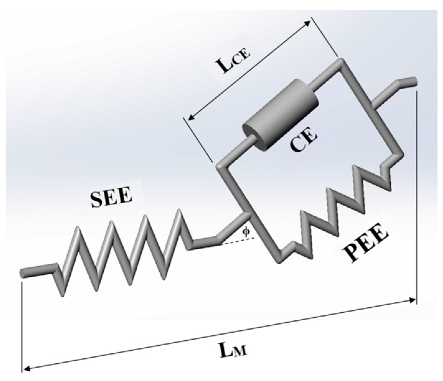
The application of mathematical models in biological systems are very powerful tools when it is wanted to model a complex system. In our case of study, muscle dynamics depends on several factors or effects that are all working at the same time, introducing a significant complexity in muscle fiber analysis. The model that is applied in the present study is mathematically defined in [13]. This model will be used due to its simplicity to be applied in control system modeling and because it is realistic enough to correctly explain the arm’s muscles dynamics.
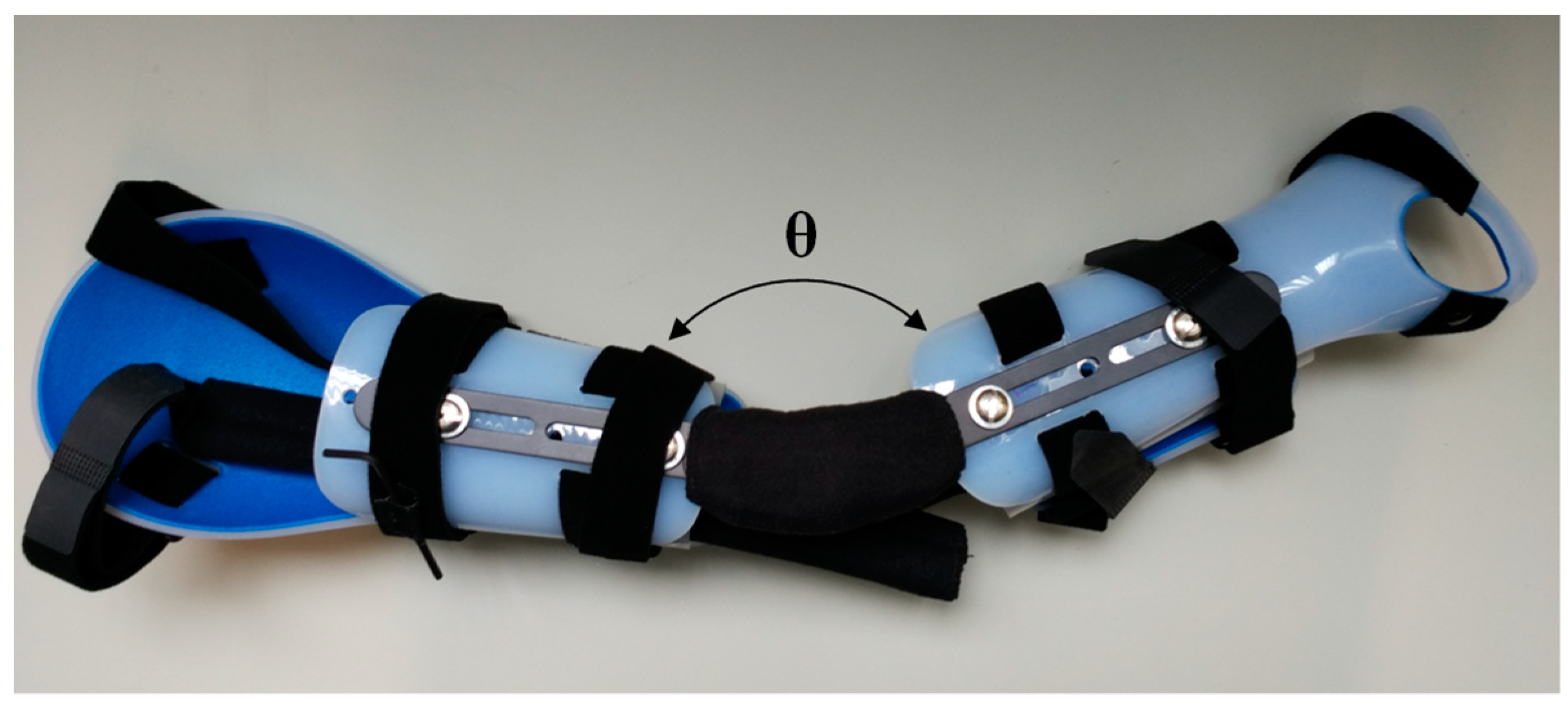
This study has been carried out in order to improve the control and movement of a robotic arm prosthesis or orthosis. We hypothesized that the application of an optimization algorithm could contribute to decreasing the necessary development force of the biceps muscle carried out for a patient to overcome a load. These man-machine interfaces have become very important for physically disabled people to carry out specific jobs or operations and they will become even more important in the future. The purpose of this orthosis is to aid people who lost the ability to move the upper arm or who lost strength in the muscles. The arm orthosis is custom made and it can be seen in Figure 1. Two surface EMG sensors and a goniometer capture the EMG signals and transmit it to a biomedical amplifier system, which transmits the amplified signals to a data acquisition card to process the signals on a computer with MATLAB software that is installed. From the computer, i the possibility to control the arm orthosis exists, which two linear actuators power.
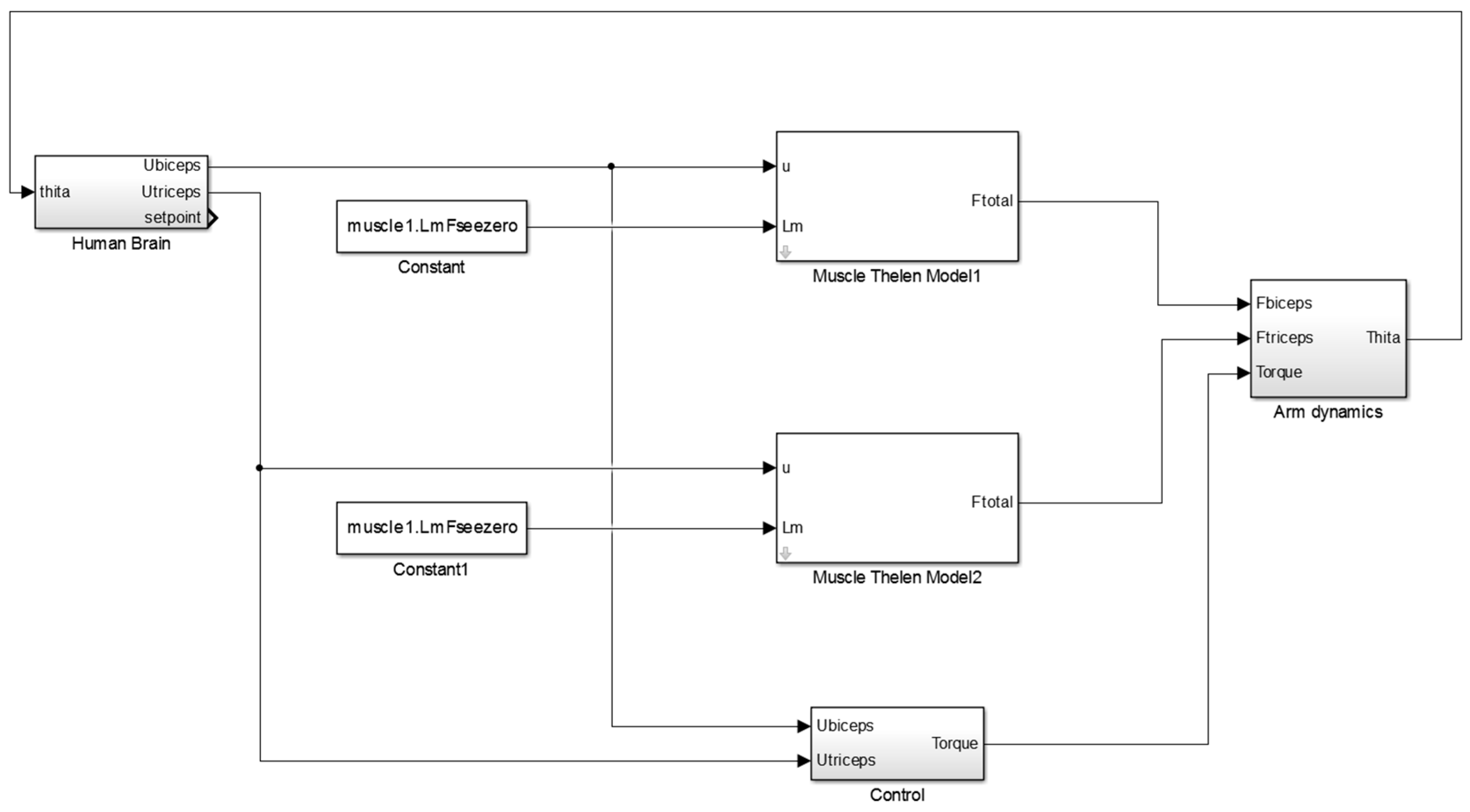
 Figure A1 of Appendix A illustrates the main Simulink diagram that is used in this study to control the orthosis.

2. Motorized Orthosis Control Problem Settlement

The proposed model is a Single Input Single Output (SISO) system. The muscle model input is a neural signal that expresses the command that is given by the human subject to activate the muscle, whereas the output signal of the model is the force that is generated by the muscle, as shown in Figure A2. This model has several parameters that are known by the literature (Chadwick et al. [13]), which have high sensibility in our system’s response. The mechanical characteristics have also high influence in this response. In this study, we have supposed that muscles only develop a force in a single direction. This assumption is good enough for control objectives. In [19], Hill defined the three element model that was presented in Figure 2; the contractile element (CE), an elastic element (PEE) in parallel connection with the contractile element, and finally another elastic element (SEE) in series connection with the contractile element. Thelen [20] adjusted the parameters of the Hill-type muscle model to reflect the observed age-related changes in dynamic muscle contractions.

2.1. Muscle-Skeletal Dynamic

This process is described by the non-linear first order differential Equation (1), as shown in the work of He et al. [21].
d a d t = ( u T a c t + 1 u T d e a c t ) ( u a )
where the activation dynamics a is the activation level of this muscle and ‘u’ is the neural excitation level that is acquired by the muscle. The activation and deactivation time constants T act   and   T deact values were obtained from the work of Winters and Stark [22]. The total force generated by the muscle, as described by Equation (2), is calculated by the mechanical model that is proposed in Figure 2.
F t o t a l = ( F a c t i v e + f P E E ( L C E ) ) c o s ϕ = f S E E ( L M L C E   c o s ϕ )
where L CE is the contractile element’s length, L M is the muscle’s length, and ϕ is the pennation angle. F active , f PEE , and f SEE correspond to the forces that are applied into CE, PEE and SEE points, respectively. The value of the pennation angle has been set to s = L CE cos ϕ in order to avoid singularity problems, as used in the work of Van den Vogert et al. [15].

2.2. Muscle Model

The contractile element active force is calculated, as shown in Equation (3):
F a c t i v e = a · F m a x · f F L ( L C E ) · f F V ( L ˙ C E )
where a is the activation level and F max is the maximum isometric force. This parameter is estimated for each muscle, where several studies in human bodies give a 100 N/cm2 value for transversal force stress (see Klein-Breteler et al. [23] and Holzbaur et al. [24]). The Gaussian like function of Equation (4) describes the mathematical relationship between the normalized force and the contractile element’s length ( L CE ).
f F L ( L C E ) = e ( L C E L C E o p t w · L C E o p t ) 2
L CE is the contractile element’s length, L CEopt its optimal length (values are given in the work of Klein-Breteler [23]), and the force versus length curve w parameter has been set to 0.56. The pennation angle and the optimal length values have been set to values that are given in [23].
f FV ( L ˙ CE ) is the force versus speed function, as defined by Equation (5), based on the mathematical expression of McLean et al. [25]:
f F V ( V C E ) { V m a x + V C E V m a x V C E A   i f   V C E 0 g m a x · V C E + c 3 V C E + c 3   i f   V C E > 0
where V CE is the contractile element’s contraction speed, the A parameter is set to 0.25 according to Herzog [26], and the maximum activation speed, V max , is set to 10 m/s. The parameter g max is assumed to be 1.5, following to [25], whereas the parameter c 3 is calculated from f FV ( V CE ) function’s first derivate when V CE = 0, as shown in Equation (6).
c 3 = V m a x · A ( g m a x 1 ) A + 1
The parallel elastic element (PEE) and series elastic element (SEE), as determined by Equation (7), are modeled as passive non linear springs:
F ( L ) { K 1 ( L L s l a c k )   i f   L   L s l a c k K 1 ( L L s l a c k ) + K 2 ( L L s l a c k ) 2     i f   L > L s l a c k
K1 term is set to 10 N/m. This value is low, but it is necessary to give some rigidity to the muscle models. Actually, a null value can generate singularity problems. The K2 term is assumed to have a null value. In SEE, the Lslack parameter, which is the length of the element when it is relaxed, is set by means of the results that were obtained in the cadaver studies, whereas, in PEE, the L CEopt value is identical with the exception of some muscle elements that support high passive forces. These values are calculated in the work of Chadwick et al. [27].

2.3. Brain Model

We have assumed that the human brain behavior can be modelled as a proportional controller in position. The signal is distributed in the ubiceps and utriceps signals, as represented in the Equations (8) and (9):
u b i c e p s ( t ) { ( θ s p θ ) K p       i f   ( θ s p θ ) 0 0   i f   ( θ s p θ ) < 0    
u t r i c e p s ( t ) { K p ( θ s p θ )   i f ( θ s p θ ) < 0 0   i f   ( θ s p θ ) 0
where θ is the angular position of the forearm, θsp is the instruction of the angular position of the forearm, and Kp is the gain between the error of the angular position and its instruction. ubiceps and utriceps are the neural excitation level of biceps and triceps, respectively. Each signal has a saturation block to remain within an interval and the utriceps signal has a negative gain, since the triceps muscles exerts a force opposed to the biceps muscle, as illustrated in Figure A3. That is, if the biceps muscle is extended, then the triceps muscle is relaxed.

2.4. Arm Model

Equation (1) has been also used, since the arm activation dynamics is similar to the muscle model. Therefore, Equations (10) and (11), along with Equation (1), describe the modeling procedure of the biceps and triceps muscles, where the fSEE force is calculated.
F T o t a l = ( F a c t i v e + f P E E ( L C E ) ) c o s ϕ = f S E E ( L M L C E   c o s ϕ )
F ( L ) { K 1 ( L L s l a c k )   i f   L   L s l a c k K 1 ( L L s l a c k ) + K 2 ( L L s l a c k ) 2     i f   L > L s l a c k
From Equations (10) and (11), we are able to obtain Equation (12):
L T = L M L C E   c o s ϕ
where LT is the length of the SEE element. Once LT is calculated, the value of fSSE is obtained and then the value of LCE. When it comes to considering the model, different options have been studied and the integration method was chosen. The LCE variable is calculated depending on two situations, as shown in Figure A4.
  • When the activation is not null, it is achieved with the inversion of the differential equation that relates the active force and the relation VCE.
  • When the activation is null, the influence of the element CE disappears. The force that is achieved as a consequence of the extinction of the CE element is the one that is only caused by the elements SEE and PEE, and this is possible when the contractile element’s length is equal to the slack length (LCE = Lslack).
The calculation of the variable LCE is achieved by means of Equations (13)–(16):
F a c t i v e = a · F m a x · f F L ( L C E ) · f F V ( L ˙ C E )
f F L ( L C E ) = e ( L C E L C E o p t w · L C E o p t ) 2
f F V ( V C E ) { V m a x + V C E V m a x V C E A   i f   V C E 0 g m a x · V C E + c 3 V C E + c 3   i f   V C E > 0
F ( L ) { K 1 ( L L s l a c k )   i f   L   L s l a c k K 1 ( L L s l a c k ) + K 2 ( L L s l a c k ) 2     i f   L > L s l a c k
Once defined the muscle model, it is necessary to describe the dynamics of the arm by means of the Equation (17), as shown in Figure A5. The momentum of inertia Jarm is obtained with the Equation (18) in order to achieve the arm dynamics.
J a r m d 2 θ d t 2 = R m u s c l e · ( F B i c e p s F T r i c e p s ) + T c o n t r o l + T l o a d
J a r m = I g + m a r m · d 2
where Ig is the forearm inertia with respect to its center of gravity, marm is the mass of the arm, and d is the distance between the mass center of the forearm and its center of rotation.
The forces FBiceps and FTriceps muscles are obtained through the Rmuscle parameter, creating a force momentum.

3. Proposed Control Scheme and Control Parameter Adjustment

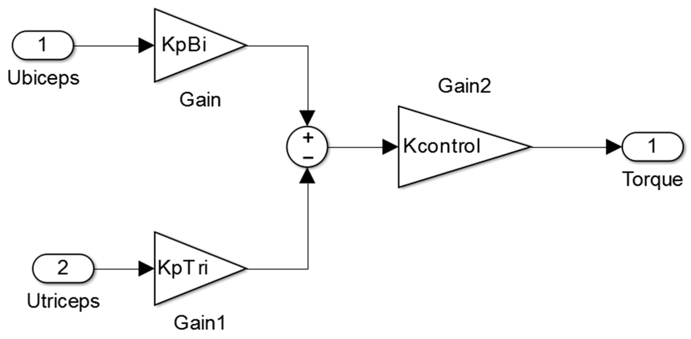
As illustrated in the control block of Figure A6, the Kpbi and Kptri gain values are calculated by the intelligent algorithm that is explained later in this study. The goal of this block is to provide the necessary assistant force to move the muscle. It is obtained with the Kpbi and Kptri gain values of the Equation (19). Kcontrol is a gain value that is set to 0.1 or to 0.3, with the aim of achieving enough torque assistance. Kpbi and K
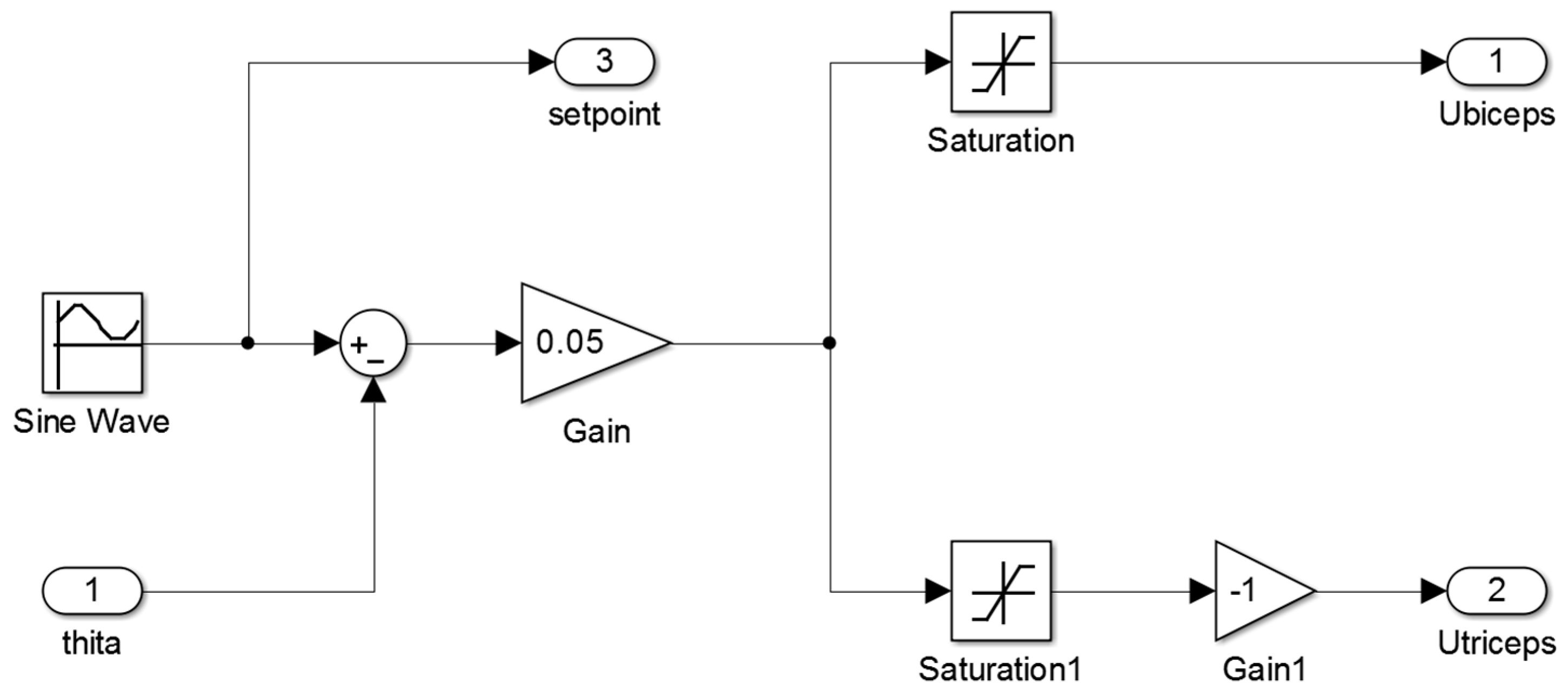
ptri are set in order to define the relative strength between the biceps and triceps EMG signals in order to achieve the best dynamics response (see Equation (20)).
T c o n t r o l = K c o n t r o l · ( K p b i · u B i c e p s K p t r i · u T r i c e p s )
The proposed control law has two inputs: ubiceps, the neural excitation level of biceps and utriceps, the neural excitation level of triceps. These two inputs, which are captured and estimated by surface EMG signal sensors, are calculated as the rectified and filtered values of surface EMG sensors located in biceps and triceps. The proportional gains models the weight of each signal in torque assistance. An intelligent optimization algorithm, as described below, must set these parameters.
The authors proposed this control, since it is simple enough to be executed by a real time processor and it takes into account the main variables that define the system state (the excitation levels of triceps and biceps). This control law does not take into account the real setpoint, because it is unknown, so the control measures the excitation level in order to know which the desired forearm angle is. Table 1 represents the parameters that were used in the proposed control scheme.

3.1. Control Parameter Optimization

A cost function has been described within the optimization algorithm by means of the Equation (20). The goal of this function is to minimize the effort that is made by the subject and to assure that the algorithm follows as close as possible the defined setpoint value.
C o s t   f u n c t i o n = α 1 ( | θ s p θ ¯ | ) + α 2   ( 1 T 0 T [ u b i c e p s ( t ) ] 2 ) + α 3   ( 1 T 0 T [ u t r i c e p s ( t ) ] 2 ) + α 4 ( m a x ( | θ s p θ | ) )
where θ is the angular position of the forearm, θsp is the instruction of the angular position of the forearm, and αj are the different weights of different relevant design criteria: the mean absolute error, the maximum absolute error, and the effort made by biceps and triceps (described by the square mean value of biceps and triceps excitations levels) and T is the time horizon.

3.2. Optimization Algorithm Description

The differential evolution (DE) is applied in the resolution of complex problems being an optimization method within the evolutionary computation. As other intelligent or swarm optimization algorithms, the DE algorithm proposes different agents set. All agents in this set are evaluated, crossed, mutated and selected. All these steps are made in order to improve the agent set.
Algorithms, the variables that are wanted to be optimized in the problem, take real values, as they were codified from a vector. The length of these vectors (n) and the quantity of variables of the problem is the same. In order to define a vector, the nomenclature x p g has been used, where p is the indicator of the individual population (p = 1…NP) and g is the corresponding generational number. The vectors are also completed with the problem variable x p , m g , where m is the indicator of the variable of the population (m = 1…n).
The problem field variables reach the minimum and maximum values at x m min and x m max , respectively. In the current case, the variables K pbi y K ptri have been limited to 50. The DE algorithm has four stages:
  • Initialization
  • Mutation
  • Recombination
  • Election
The initialization algorithm is executed each time that it takes place. However, the mutation, recombination, and election algorithms are indefinitely repeated until one of the next elements is satisfied (the generational quantity, the past time, the quality of the solution achieved). The function of each one of these stages is explained below.

3.2.1. Initialization

The population is randomly initialized, while taking into account the maximum and minimum values of each variable, as described in Equation (21):
x p , m 1 = x m m i n + r a n d ( 0 , 1 ) · ( x m m a x x m m i n )  
where p = 1…NP, m = 1…n and rand(0,1), (0,1) is any value of the interval.

3.2.2. Mutation

The mutations NP have as a goal the origin of the vectors. These vectors are created choosing three elements (xa, xb, xc), and they are achieved with the Equation (22):
n p t = x c + F · ( x a x b )  
where a, b, and c cannot be the same value and p = 1…NP. F is a parameter that controls the mutation rate founded in the interval (0,2).

3.2.3. Recombination

When the random vectors NP have been obtained, their recombination is also randomly carried out in comparison with the original vectors (xp,g). In this way, the new agent proposal ( t m g ) is achieved by Equation (23):
t p , m g { n p , m g   i f   r a n d ( [ 0 , 1 ] ) < G R x p , m g   i f   a n y   o t h e r   c a s e
where p = 1…NP, m = 1…n and GR is the parameter that controls the recombination rate. Subsequently, a variable-variable comparison is carried out, thus, the test vector NP can be considered as a mixture between the vectors and the original vectors.

3.2.4. Election

In the election process, the cost function is calculated by means of the element that is achieved in the recombination. From this value, it is compared with the value of the function that is wanted to be represented and it will get with the cost that provides the best value.

4. Results and Discussion

Table 2 summarized the three different cases that have been simulated, depending on the application of the optimization algorithm and the addition of a load, respectively.
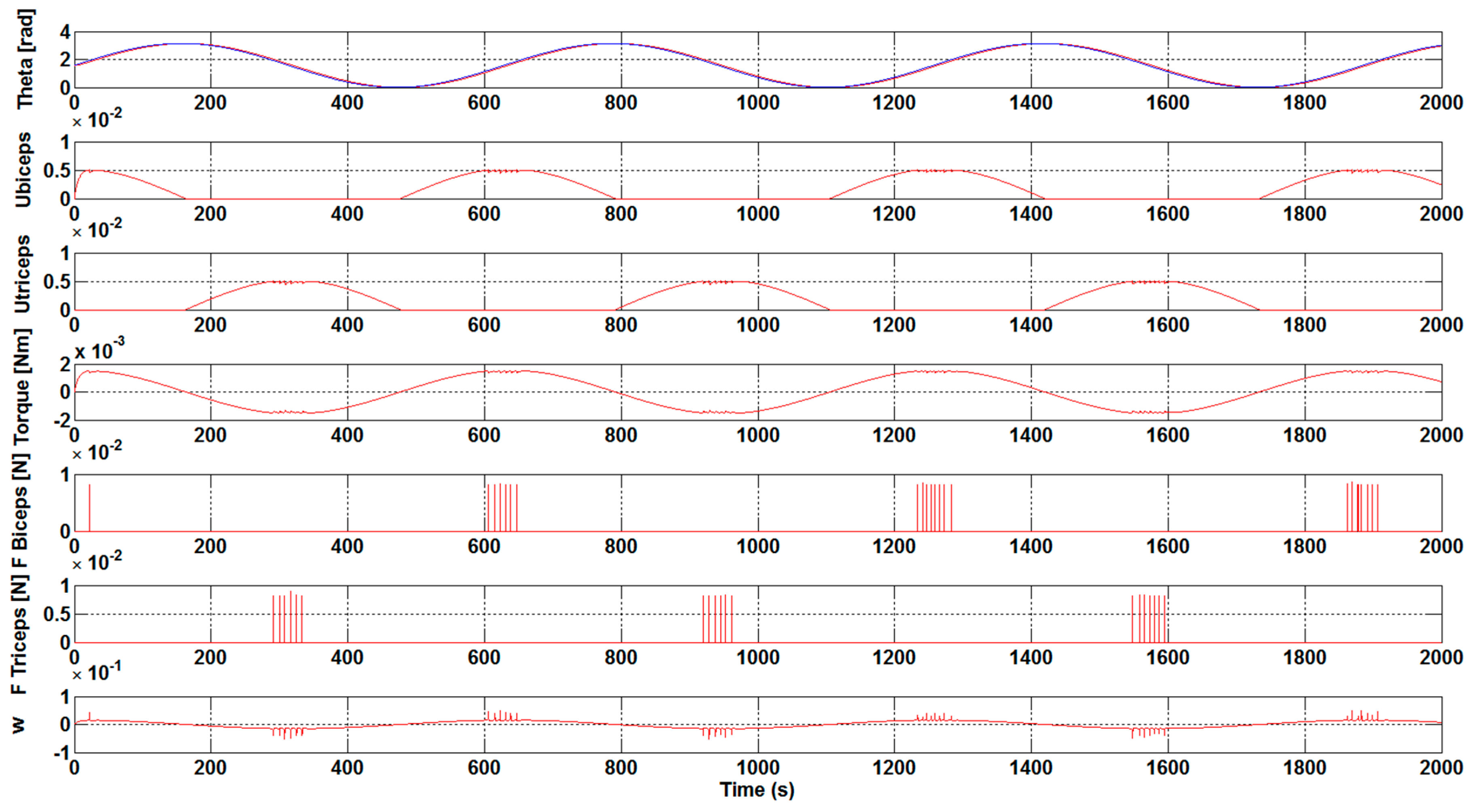
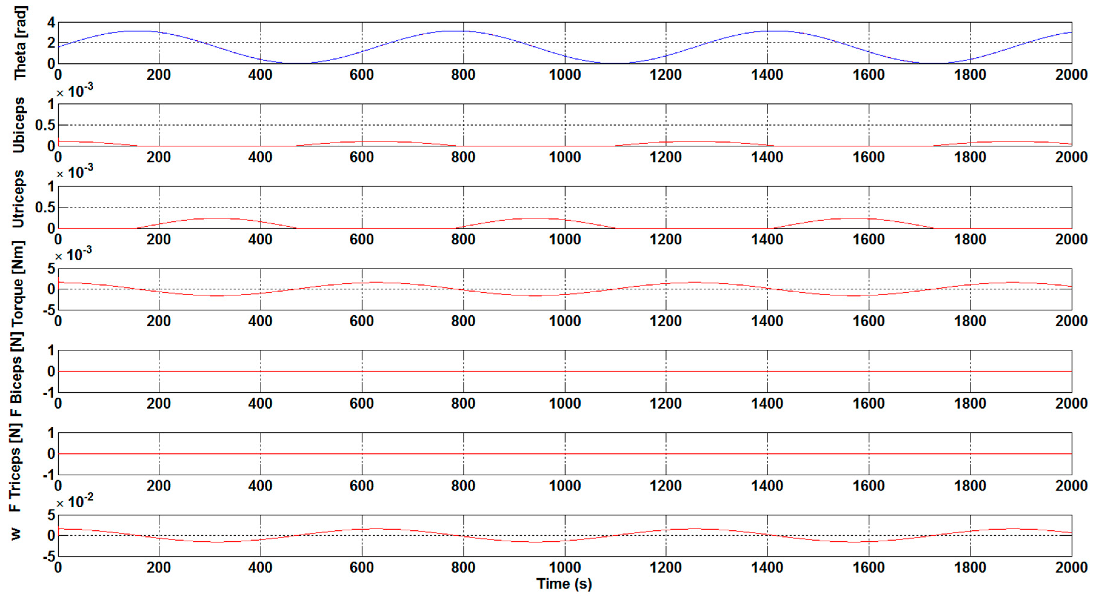
The results that are presented in Figure 3 and Figure 4 correspond to a case without the optimization algorithm described earlier and they were obtained with a Kcontrol gain value of 0.1 and 0.3, respectively. The first subplot shows the θ and θsp forearm angle values and how the reference signals continue in a suitable way. The following two subplots illustrate the ubiceps and utriceps signals. As previously mentioned, these muscles are antagonistic, so, when one of these muscles is activated, the other is deactivated and vice versa. Subsequently, the subplots with FBiceps and FTriceps are represented, which express the force value of each muscle when they are activated. Finally, the subplot with w represents the arm angular velocity (rad/s).
Analyzing the results, it was observed that an increase in the Kcontrol gain value leads to a decrease in the effort that is necessary to bear the weight of the arms. This behavior was expected, since we are assisting the arm by means of the gain, and therefore the force that is necessary to carry out the movements is reduced.
Currently, the DE algorithm has been executed to calculate the optimum gain value K pbi and K ptri . In our case, 100 particles and 100 iterations have been used to carry out this calculation and the gain values have been limited between 0 and 50. The best results are achieved with the maximum Kcontrol gain value, according to the Fbiceps and Ftriceps values of Figure 3 and Figure 4, that is, the force that is made by the muscle from the beginning to carry out the movements is lower. Subsequently, the previous data and the optimum gain values K pbi and K ptri are used.
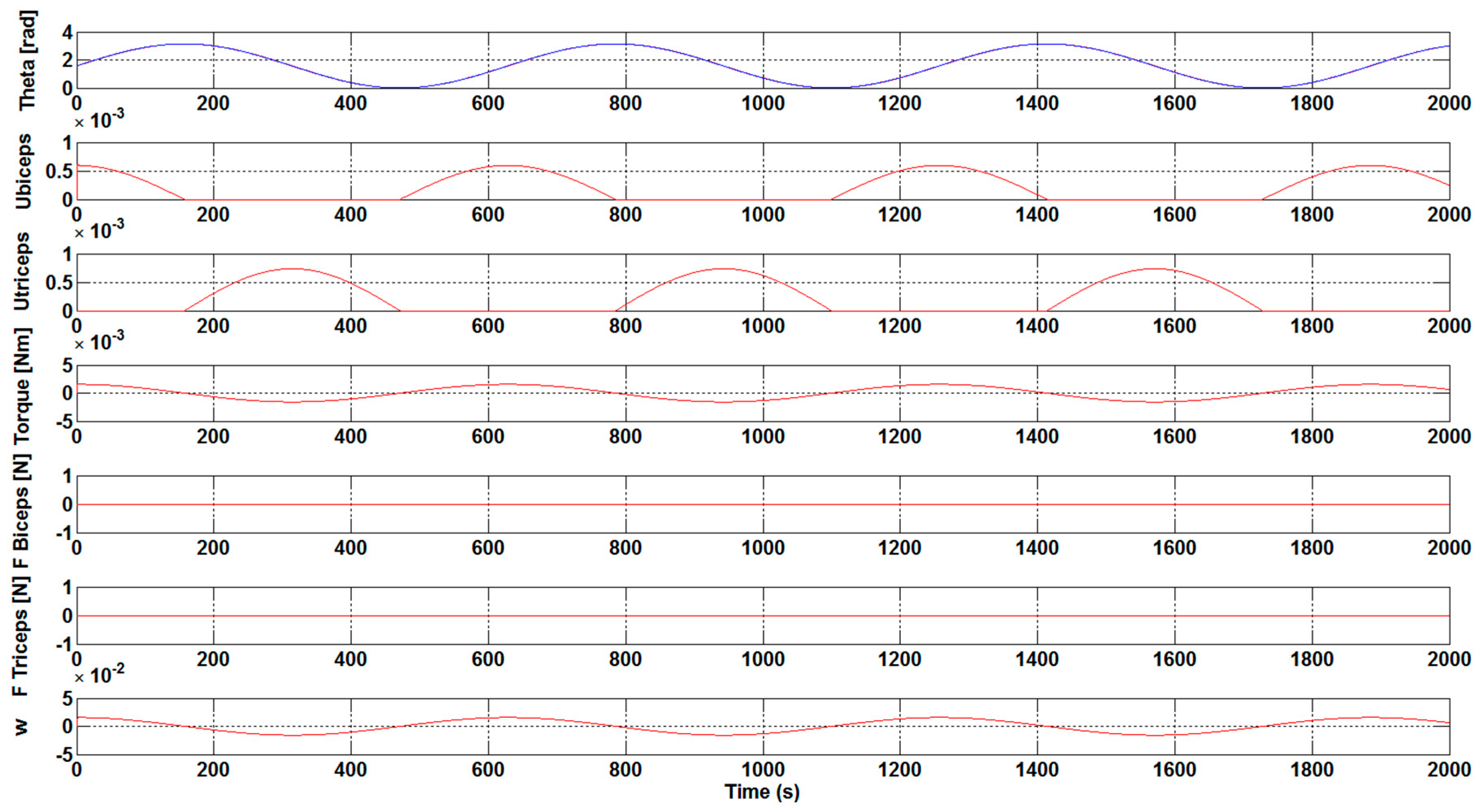
Once analyzing the results that were obtained in Figure 5 and Figure 6, it is clearly visible that the necessary development force of the muscles, FBiceps and FTriceps, is very low, close to zero. It is also clear that the ubiceps and utriceps signal values are getting lower with a Kcontrol gain increase. Taking into account the aforementioned, the optimum Kpbi and Kptri gain values have great importance for the muscles to do less effort when it comes to making any movement.
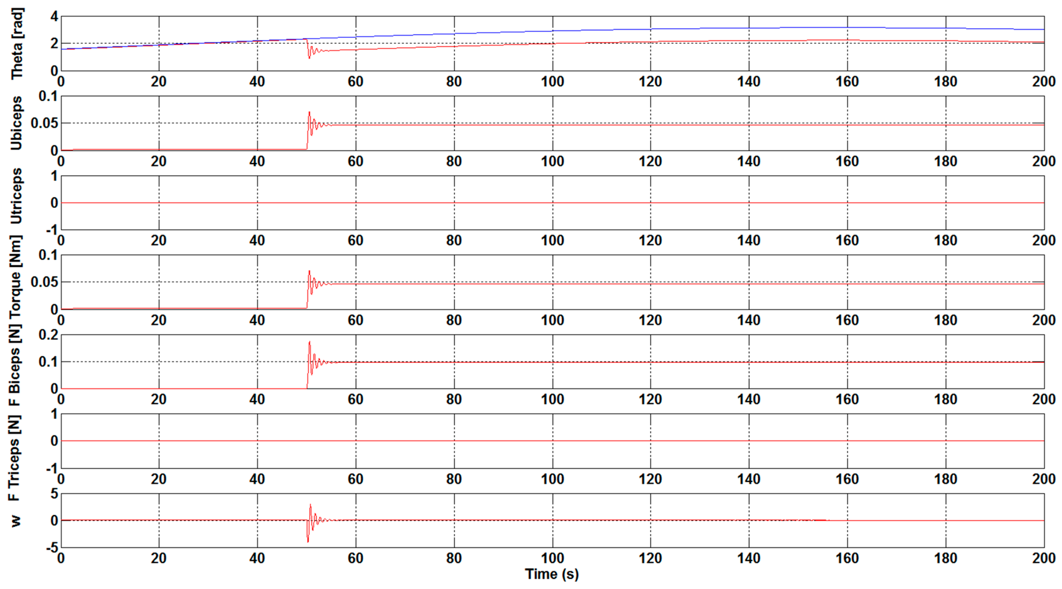
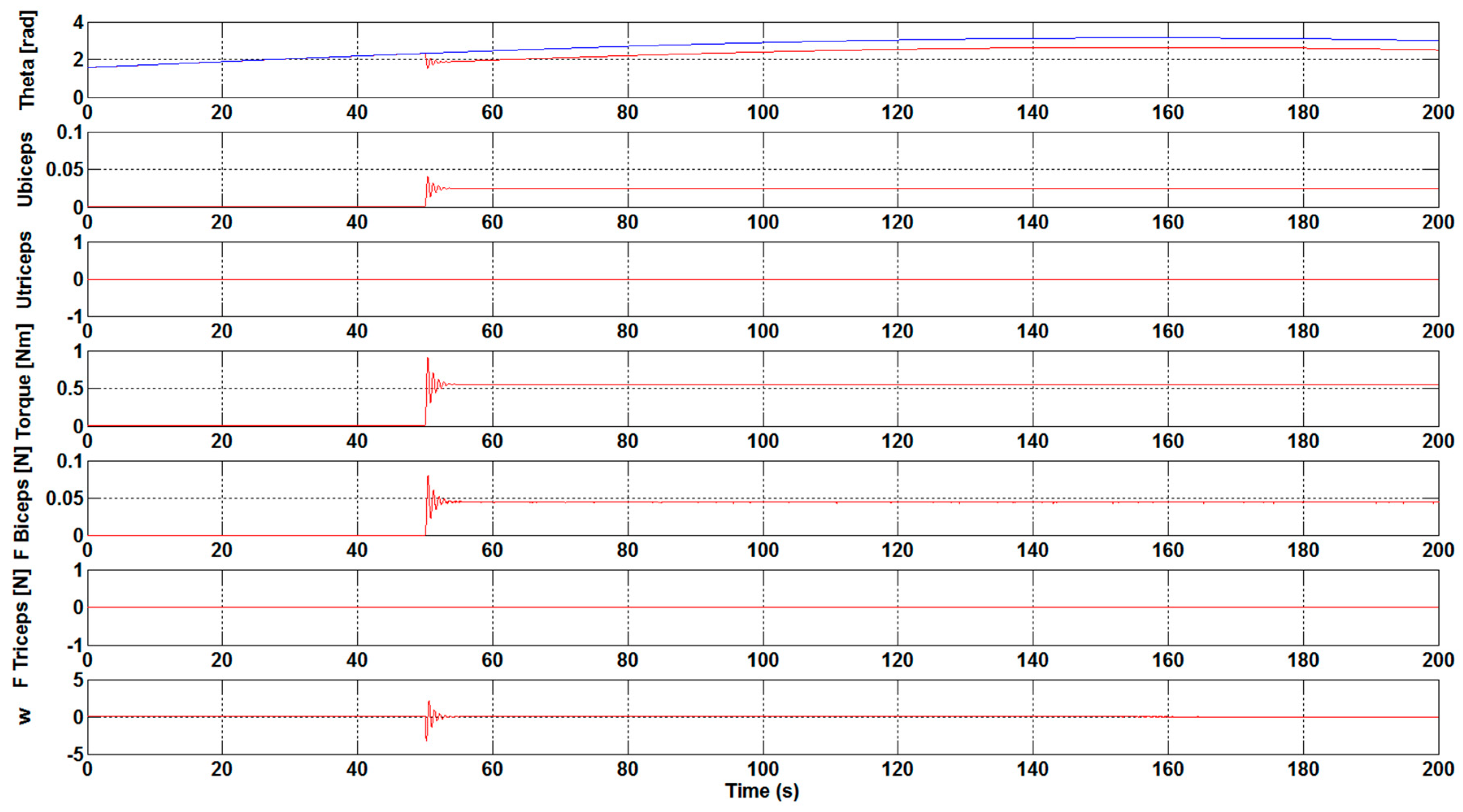
The next step has been to introduce a load to the control system of the orthosis in order to study the necessary force that is to be carried out by the biceps. As shown in Figure 7 and Figure 8, a load of 1 N·m was introduced 50 seconds after the simulation starts. The results show the perturbation produced when the load is applied. Furthermore, the results show how, without the optimization algorithm, the required development force of the biceps muscle to overcome the load is practically double with respect to the case with the optimization algorithm. Specifically, a value of 0.1 N has been achieved for FBiceps without applying the optimization algorithm, as illustrated in Figure 7. However, when the optimization algorithm has been used a value of 0.05 N has been obtained, see Figure 8.
It was observed that an increase in the Kcontrol gain value led to a decrease in the effort that is necessary to bear the weight of the arms. With the execution of the DE algorithm to calculate the optimum gain values, K pbi and K ptri , it was clearly visible that the necessary development force of the muscles is very small, being close to zero. Additionally, the ubiceps and utriceps signal values were getting lower, with a gain increase highlighting the importance of the optimum gain values for the muscles in order to carry out less effort. The introduction of a load in the control system showed that the necessary development force of the biceps muscle to overcome the load is practically the double with respect to the case with the optimization algorithm without the optimization algorithm.
The major novelty of the current research is the implementation of an optimization algorithm based on differential evolution (DE) to improve the control and movement of the orthosis. This method, which is based on evolutionary principles, has been chosen due to its simplicity, small number of configuration parameters, and good performance. Sanz-Merodio et al. [28] combined the use of different gains and passive elements to reduce the energy consumption while applying a static optimization. Additionally, Belkadi et al. [29] proposed a PID adaptive controller based on modified particle swarm optimization algorithm, where the controller is initialized with the desired position and velocity instead of EMG signals, as made in this work. Experimental studies, as the one carried out with eight subjects by Song et al. [30], showed improvements in the upper limb functions with the use of a controlled robotic system with one degree-of-freedom. Recently, in the study of McCabe et al. [31], a clinical case of an upper limb orthosis can be found for use in assisting the user to perform the flexion/extension of the elbow demonstrating the feasibility of the implementation of an upper limb myoelectric orthosis. Stein et al. [32] developed a novel device, the Active Joint Brace (AJB), which combined an exoskeletal robotic brace with EMG control algorithms. They confirmed the feasibility of using an EMG-controlled powered exoskeletal orthosis for exercise training. The control and optimization algorithm that was carried out in the current research to assist the elbow movement could contribute to the improvement of devices as the one studied by Page et al. [33], which enables the bidirectional control at the elbow into flexion or extension. New wearable devices, as the one developed by Rong et al. [34], combining a neuromuscular electrical stimulation (NMES) and robot hybrid system, have also showed improvements in the coordination of agonist/antagonist pairs when performing sequencing limb movements.
In the previous study that was made by Suberbiola et al. [17], a similar EMG based orthosis control was proposed. However, this work did not explain how the control parameters can be obtained. Recently, Dao et al. [35] developed a modified computed torque controller to enhance the tracking performance of a robotic orthosis of the lower limb. Their control laws proposed have similar concepts, but with different objectives and approaches. In the current study, we follow the movements of the human being, whereas, in [35], they try to teach or show the correct forces and torques that must be applied to follow the desired trajectory.

5. Conclusions

Computational methods are tools quite useful and powerful for making a test of the muscle unit. These procedures are more comfortable and less expensive in comparison with the experimental method. In the present study, a numerical model of a muscle, arm, and orthosis has been developed and different cases have been tested.
The optimum gain values that were obtained with the DE optimization algorithm, K pbi and K ptri , showed necessary development forces close to zero, which highlighted the importance of these values for the muscles to carry out less effort. Improvements were also observed with the introduction of a load of 0.1 N and the application of the DE optimization algorithm, where practically half of the development biceps force was necessary to overcome the load.
An important contribution of the present study has been the implementation of a numerical model of a muscle, arm, and orthosis. In this case, a singularity was created when the activation took a value of zero. In fact, the muscle was deactivated and the arm stayed without force when the activation was null. However, the singularity has been avoided, because the force of the serial element does not take immediately the zero value. Thus, even though the activation was zero, the muscle force does not immediately drop to zero. Additionally, an intelligent optimization system has been developed in order to calculate the value of two important non-linear parameters,   K pbi and K ptri , in the orthosis control law.

Author Contributions

I.A., E.Z. and U.F.-G. performed the new control algorithm and carried out the Formal Analysis. D.T.-F.-B. and A.S.-A. supervised the methodology and contributed to the preparation and creation of the manuscript.

Funding

The authors are grateful to the Government of the Basque Country and the University of the Basque Country UPV/EHU through the SAIOTEK (S-PE11UN112) and EHU12/26 research programs, respectively. The Regional Development Agency of the Basque Country (SPRI) is gratefully acknowledged for economic support through the research project KK-2018/00109, ELKARTEK.

Acknowledgments

This research was partially funded by Fundation VITAL Fundazioa.

Conflicts of Interest

The authors declare no conflict of interest.

Appendix A

Figure A1. General Simulink diagram used in the orthosis control.
Applsci 09 02453 g0a1
Figure A2. Implementation of Thelen Model.
Applsci 09 02453 g0a2
Figure A3. Human Brain’s behavior model.
Applsci 09 02453 g0a3
Figure A4. Block diagram representing the contractile element’s length (Lce).
Applsci 09 02453 g0a4
Figure A5. Arm dynamics model.
Applsci 09 02453 g0a5
Figure A6. Control law proposal. The optimum K pbi and K ptri values are calculated through the optimization algorithm.
Applsci 09 02453 g0a6

References

  1. Dollar, A.M.; Herr, H. Lower extremity exoskeletons and active orthoses: Challenges and state-of-the-art. IEEE Trans. Robot. 2008, 24, 144–158. [Google Scholar] [CrossRef]
  2. Lo, H.S.; Xie, S.Q. Exoskeleton robots for upper-limb rehabilitation: State of the art and future prospects. Med. Eng. Phys. 2012, 34, 261–268. [Google Scholar] [CrossRef] [PubMed]
  3. Kiguchi, K.; Hayashi, Y. An EMG-Based Control for an Upper-Limb Power-Assist Exoskeleton Robot. IEEE Trans. Syst. Man Cybern. Part B Cybern. 2012, 42, 1064–1071. [Google Scholar] [CrossRef] [PubMed]
  4. Van der Heide, L.A.; van Ninhuijs, B.; Bergsma, A.; Gelderblom, G.J.; van der Pijl, D.J.; de Witte, L.P. An overview and categorization of dynamic arm supports for people with decreased arm function. Prosthet. Orthot. Int. 2014, 38, 287–302. [Google Scholar] [CrossRef] [PubMed]
  5. ISO. 9999 Assistive Products for Persons with Disability—Classification and Terminology; ISO: Geneva, Switzerland, 2011. [Google Scholar]
  6. Tsagarakis, N.; Caldwell, D. Development and control of a ‘soft-actuated’ exoskeleton for use in physiotherapy and training. Auton. Robot. 2003, 15, 21–33. [Google Scholar] [CrossRef]
  7. Kiguchi, K.; Tanaka, T.; Fukuda, T. Neuro-fuzzy control of a robotic exoskeleton with EMG signals. IEEE Trans. Fuzzy Syst. 2004, 12, 481–490. [Google Scholar] [CrossRef]
  8. Pratt, J.; Krupp, B.; Morse, C.; Collins, S. The RoboKnee: An exoskeleton for enhancing strength and endurance during walking. In Proceedings of the 2004 IEEE International Conference on Robotics and Automation, New Orleans, LA, USA, 26 April–1 May 2004; pp. 2430–2435. [Google Scholar] [CrossRef]
  9. Peternel, L.; Noda, T.; Petric, T.; Ude, A.; Morimoto, J.; Babic, J. Adaptive Control of Exoskeleton Robots for Periodic Assistive Behaviours Based on EMG Feedback Minimisation. PLoS ONE 2016, 11, e0148942. [Google Scholar] [CrossRef]
  10. Cavallaro, E.E.; Rosen, J.; Perry, J.C.; Burns, S. Real-time myoprocessors for a neural controlled powered exoskeleton arm. IEEE Trans. Biomed. Eng. 2006, 53, 2387–2396. [Google Scholar] [CrossRef]
  11. Tang, Z.; Zhang, K.; Sun, S.; Gao, Z.; Zhang, L.; Yang, Z. An Upper-Limb Power-Assist Exoskeleton Using Proportional Myoelectric Control. Sensors 2014, 14, 6677–6694. [Google Scholar] [CrossRef] [Green Version]
  12. Williams, M.R. A pilot study into reaching performance after severe to moderate stroke using upper arm support. PLoS ONE 2018, 13, e0200787. [Google Scholar] [CrossRef]
  13. Chadwick, E.K.; Blana, D.; Kirsch, R.F.; van den Bogert, A.J. Real-Time Simulation of Three-Dimensional Shoulder Girdle and Arm Dynamics. IEEE Trans. Biomed. Eng. 2014, 61, 1947–1956. [Google Scholar] [CrossRef] [PubMed] [Green Version]
  14. Chadwick, E.K.; Blana, D.; Simeral, J.D.; Lambrecht, J.; Kim, S.P.; Cornwell, A.S.; Taylor, D.M.; Hochberg, L.R.; Donoghue, J.P.; Kirsch, R.F. Continuous neuronal ensemble control of simulated arm reaching by a human with tetraplegia. J. Neural Eng. 2011, 8, 034003. [Google Scholar] [CrossRef]
  15. Van den Bogert, A.J.; Blana, D.; Heinrich, D. Implicit methods for efficient musculoskeletal simulation and optimal control. Procedia IUTAM 2011, 2, 297–316. [Google Scholar] [CrossRef] [Green Version]
  16. Tsai, A.; Hsieh, T.; Luh, J.; Lin, T. A comparison of upper-limb motion pattern recognition using EMG signals during dynamic and isometric muscle contractions. Biomed. Signal Process. Control 2014, 11, 17–26. [Google Scholar] [CrossRef]
  17. Suberbiola, A.; Zulueta, E.; Manuel Lopez-Guede, J.; Etxeberria-Agiriano, I.; Grana, M. Arm Orthosis/Prosthesis Movement Control Based on Surface EMG Signal Extraction. Int. J. Neural Syst. 2015, 25, 1550009. [Google Scholar] [CrossRef] [PubMed]
  18. Desplenter, T.; Trejos, A.L. Evaluating Muscle Activation Models for Elbow Motion Estimation. Sensors 2018, 18, 1004. [Google Scholar] [CrossRef] [PubMed]
  19. Hill, A. The heat of shortening and the dynamic constants of muscle. Proc. R. Soc. Ser. B Biol. Sci. 1938, 126, 136–195. [Google Scholar] [CrossRef]
  20. Thelen, D. Adjustment of muscle mechanics model parameters to simulate dynamic contractions in older adults. J. Biomech. Eng. Trans. ASME 2003, 125, 70–77. [Google Scholar] [CrossRef]
  21. He, J.; Levine, W.; Loeb, G. Feedback Gains for Correcting Small Perturbations to Standing Posture. IEEE Trans. Autom. Control 1991, 36, 322–332. [Google Scholar] [CrossRef]
  22. Winters, J.; Stark, L. Analysis of Fundamental Human Movement Patterns through the Use of In-Depth Antagonistic Muscle Models. IEEE Trans. Biomed. Eng. 1985, 32, 826–839. [Google Scholar] [CrossRef]
  23. Breteler, M.; Spoor, C.; Van der Helm, F. Measuring muscle and joint geometry parameters of a shoulder for modeling purposes. J. Biomech. 1999, 32, 1191–1197. [Google Scholar] [CrossRef]
  24. Holzbaur, K.; Murray, W.; Delp, S. A model of the upper extremity for simulating musculoskeletal surgery and analyzing neuromuscular control. Ann. Biomed. Eng. 2005, 33, 829–840. [Google Scholar] [CrossRef] [PubMed]
  25. McLean, S.; Su, A.; van den Bogert, A. Development, and validation of a 3-D model to predict knee joint loading-during, dynamic movement. J. Biomech. Eng. Trans ASME 2003, 125, 864–874. [Google Scholar] [CrossRef] [PubMed]
  26. Herzog, W. Muscle. In Biomechanics of the Musculoskeletal System, 2nd ed.; Nigg, M., Herzog, W., Eds.; Wiley: New York, NY, USA, 1999; pp. 148–188. [Google Scholar]
  27. Chadwick, E.K.; Blana, D.; van den Bogert, A.J.; Kirsch, R.F. A Real-Time, 3-D Musculoskeletal Model for Dynamic Simulation of Arm Movements. IEEE Trans. Biomed. Eng. 2009, 56, 941–948. [Google Scholar] [CrossRef]
  28. Sanz-Merodio, D.; Cestari, M.; Carlos Arevalo, J.; Garcia, E. Control Motion Approach of a Lower Limb Orthosis to Reduce Energy Consumption Regular Paper. Int. J. Adv. Robot. Syst. 2012, 9, 232. [Google Scholar] [CrossRef]
  29. Belkadi, A.; Oulhadj, H.; Touati, Y.; Khan, S.A.; Daachi, B. On the robust PID adaptive controller for exoskeletons: A particle swarm optimization based approach. Appl. Soft Comput. 2017, 60, 87–100. [Google Scholar] [CrossRef]
  30. Song, R.; Tong, K.; Hu, X.; Li, L. Assistive control system using continuous myoelectric signal in robot-aided arm training for patients after stroke. IEEE Trans. Neural Syst. Rehabil. Eng. 2008, 16, 371–379. [Google Scholar] [CrossRef]
  31. Mccabe, J.P.; Henniger, D.; Perkins, J.; Skelly, M.; Tatsuoka, C.; Pundik, S. Feasibility and clinical experience of implementing a myoelectric upper limb orthosis in the rehabilitation of chronic stroke patients: A clinical case series report. PLoS ONE 2019, 14, e0215311. [Google Scholar] [CrossRef] [PubMed]
  32. Stein, J.; Narendran, K.; McBean, J.; Krebs, K.; Hughes, R. Electromyography-controlled exoskeletal upper-limb-powered orthosis for exercise training after stroke. Am. J. Phys. Med. Rehabil. 2007, 86, 255–261. [Google Scholar] [CrossRef]
  33. Page, S.J.; Hill, V.; White, S. Portable upper extremity robotics is as efficacious as upper extremity rehabilitative therapy: A randomized controlled pilot trial. Clin. Rehabil. 2013, 27, 494–503. [Google Scholar] [CrossRef] [PubMed]
  34. Rong, W.; Li, W.; Pang, M.; Hu, J.; Wei, X.; Yang, B.; Wai, H.; Zheng, X.; Hu, X. A Neuromuscular Electrical Stimulation (NMES) and robot hybrid system for multi-joint coordinated upper limb rehabilitation after stroke. J. NeuroEng. Rehabil. 2017, 14, 34. [Google Scholar] [CrossRef] [PubMed]
  35. Dao, Q.; Yamamoto, S. Assist-as-Needed Control of a Robotic Orthosis Actuated by Pneumatic Artificial Muscle for Gait Rehabilitation. Appl. Sci. 2018, 8, 499. [Google Scholar] [CrossRef]
Figure 1. Custom made arm orthosis used in the present study, where θ represents the forearm angle.
Applsci 09 02453 g001
Figure 2. Hill muscle model.
Applsci 09 02453 g002
Figure 3. Results without the optimization algorithm and with a Kcontrol gain value of 0.1.
Applsci 09 02453 g003
Figure 4. Results without the optimization algorithm and with a Kcontrol gain value of 0.3.
Applsci 09 02453 g004
Figure 5. Results with the optimization algorithm and with a Kcontrol gain value of 0.1.
Applsci 09 02453 g005
Figure 6. Results with the optimization algorithm and with a Kcontrol gain value of 0.3.
Applsci 09 02453 g006
Figure 7. Results without the optimization algorithm and with the application of a load.
Applsci 09 02453 g007
Figure 8. Results with the optimization algorithm and with the application of a load.
Applsci 09 02453 g008
Table 1. Parameter values used in the proposed control scheme.
ParameterValueUnits
Human height (h)1.90m
Human weight (M)100kg
Distance (d)0.0725 × Hm
Turning radius (Rg)0.303 × dm
Arm weight (marm)0.016 × Mkg
Moment of inertia (Ig)marm × (Rg)2kg × m2
Forearm moment of inertia (Jarm)Jarm = Ig + marm × (d2)kg/m2
Arm length (Rarm)Rarm = 2 × d/10m
Friction coefficient0.1N·m/rad·s
Table 2. Test cases studied for the orthosis control system.
Without LoadWith Load
No optimization algorithm1. Comparison between a Kcontrol value of 0.1 and 0.3, respectively3. Comparison between a case without the optimization algorithm and with the application of the optimization algorithm
Optimization algorithm activated2. Comparison between a Kcontrol value of 0.1 and 0.3, respectively

