Unobtrusive Respiratory Flow Monitoring Using a Thermopile Array: A Feasibility Study

Abstract

Low-resolution thermal cameras have already been used in the detection of respiratory flow. However, microbolometer technology has a high production cost compared to thermopile arrays. In this work, the feasibility of using a thermopile array to detect respiratory flow has been investigated in multiple settings. To prove the concept, we tested the detector on six healthy subjects. Our method automatically selects the region-of-interest by discriminating between sensor elements that output noise and flow-induced signals. The thermopile array yielded an average root mean squared error of $1.59breathsperminute$. Parameters such as distance, breathing rate, orientation, and oral or nasal breathing resulted in being fundamental in the detection of respiratory flow. The paper provides the proof-of-concept that low-cost thermopile-arrays can be used to monitor respiratory flow in a lab setting and without the need for facial landmark detection. Further development could provide a more attractive alternative for the earlier bolometer-based proposals.

1. Introduction

Continuous respiratory monitoring can be used to predict potentially serious clinical events like cardiopulmonary arrest [1,2], and it is particularly relevant for the detection of specific clinical conditions such as apnea of prematurity, Sleep Disordered Breathing (SDB), or Sudden Infant Death Syndrome (SIDS) [3]. Respiratory activity can be monitored with a variety of techniques including flow sensors, chest wall motion sensors, and indirect extraction of the respiration signal [2]. However, in some applications, flow sensors are necessary. In particular, obstructive apnea is a type of apnea characterized by the presence of chest wall motion, but absence of flow [4].

Various sensors can be used to detect respiration flow such as pneumotachographs, oro-nasal thermistors, or nasal pressure transducers. These, however, need to be positioned close to the nostrils, fixed on the upper lip, or integrated in a mask and result in being particularly uncomfortable for patients [4].

Many remote sensing technologies have been used to monitor respiration, e.g., RGB and near-infrared cameras or radars. Their detection is, however, based on respiration motion, not flow. An unobtrusive way to monitor respiration flow is based on thermal imaging, also called InfraRed Thermography (IRT) [5,6]. Most of the work on IRT uses the nostrils and/or the mouth area as the Region Of Interest (ROI) to evaluate the thermal induced respiratory variations. The ROI can be determined manually or automatically by using anatomical characteristics, e.g., medial canthus region, combined with tracking algorithms [7,8,9].

In real applications, e.g., sleep monitoring, multiple cameras would be necessary to monitor the patient continuously and cover all possible orientations. This would undoubtedly raise the cost of the solution, making it even more important to find an inexpensive sensor solution to detect respiration (and the absence of it).

Cho et al. [10], for example, used FLIR ONE to detect respiration flow in outdoor and indoor settings. The work focused on the robustness to environmental thermal dynamics. Whereas, Scebba et al. [11] proposed a sensor fusion of FLIR Lepton and RGB cameras. Both works were based on facial landmark detection and used relatively small microbolometer-based thermal cameras. Microbolometers are the most common sensors for uncooled infrared imaging: the infrared radiation absorbed changes the resistance of the material.

Thermopile arrays, instead, consist of multiple thermopile sensors. These sensors are constituted by thermocouples in series, which are based on the Seebeck effect, i.e., they generate a voltage proportional to the infrared radiation absorbed [12]. They have been widely used for non-contact thermometers [13], fall detection [14], human detection [15,16,17], and fever screening [18]. Thermal cameras based on microbolometers started having smaller dimensions and cost, as FLIR ONE or FLIR Lepton. However, the main difference between thermopiles and microbolometers lies in the production cost; microbolometer-based infrared imagers require several costly processes (e.g., know-how of micromachining, vacuum packaging, and materials’ preparation) that significantly raise the price [19].

It would therefore be of interest to understand if a thermopile array could be used as a respiratory flow detector, yielding a further reduction in cost. Moreover, the detection of facial landmarks is not straightforward in real environments [20], especially when the resolution would be further reduced. Recent work from Pereira et al. [20] proved the usability of a thermal camera to detect the respiration signal without the use of anatomical features, both on healthy adults and infants in the Neonatal Intensive Care Unit (NICU). The method uses a black-box approach, wherein the resolution is reduced by averaging multiple pixels. Moreover, an empirical Signal Quality Index (SQI) is used to analyze the spectrum of each cell, and the ROI containing respiratory information is chosen based on the SQI value. In the data used, both face and torso are included in the field of view, as specified in a previous work where the same dataset was used [21]. The respiration signal detected is a combination of motion-related breathing (due to shoulder motion) and thermal changes due to respiration flow. The proposed approach eliminates the need of ROI selection based on facial features. However, an unconstrained combination of motion and flow-related information is not desirable and should not be trusted in environments where apneas and, in particular, obstructive apneas are common.

In this paper, we present an unobtrusive respiration monitoring technique that uses a thermopile array and an ROI detection method that does not require facial landmarks’ visibility. To our knowledge, this is the first work that aims to use thermopile arrays to detect respiratory flow. In this study, we assess the accuracy of the breathing signal detection in the optimal stationary condition on healthy adults in a laboratory environment as a proof-of-concept.

The technique has been tested on multiple healthy subjects. Moreover, to prove the feasibility of detecting respiration with a thermopile array for typical respiration conditions, oral/nasal breathing and different Respiration Rates (RRs) have been analyzed. Furthermore, several other factors like distance from the sensor and orientation have been considered to mimic real-world applications.

The rest of the paper is organized as follows, Section 2 introduces the background and the main challenges and contains the processing steps and the experimental setup. The results and discussion will be presented respectively in Section 3 and Section 4. Finally, Section 5 provides the conclusions.

2. Materials and Methods

2.1. Background and Challenges

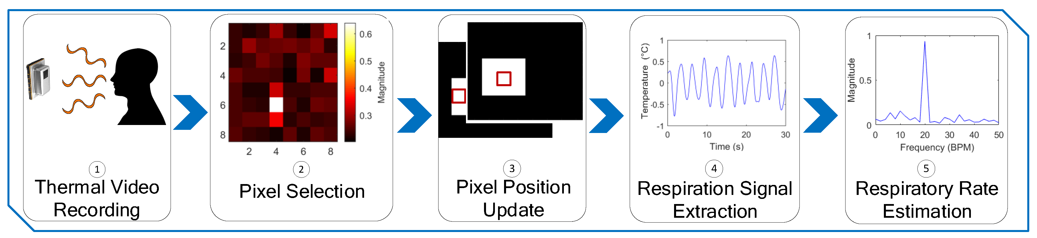
Modern thermal cameras have a sensitivity in the order of ${10}^{-2}$ K [22]. However, a typical thermopile array can only provide a sensitivity in the order of ${10}^{-1}$ K. Considering that the thermal variations in both adults and neonates have been reported to be higher than tenths of a Kelvin [23], such a sensitivity should be theoretically sufficient for the detection of flow.

The detection of respiration flow through thermal sensing is not only dependent on the amplitude of the thermal variation. Sensor characteristics also contribute to determining the ability to detect such changes.

The partial area effect [24] is a known dependency that describes the relationship between the real amplitude (temperature in this case), field of view, number of pixels, distance, size of the target, and the amplitude (temperature) detected by a sensor. It follows that the target size, i.e., the surface involved in thermal heat exchange, is an important parameter in the detection of flow. For example, differences are expected if the measurements are taken in frontal view, i.e., subject facing the device, or side view, with the head on a pillow. In the second case, the pillow material will also take part in the heat exchange process, increasing the area involved. This phenomenon was already observed by Abbas et al. [9]. The partial area effect is particularly important in sensors with a broad field of view and a low number of pixels and limits the distance of usage.

Another challenge can be found in the RR, higher RR will result in lower temperature variation due to the heat capacity. Moreover, oral and nasal respiration show differences in temperature and humidity content depending on the environment. In particular, oral exhaled air results in having a higher temperature compared to the nasal one with an ambient temperature of 20 °C [25].

A single thermal sensing element equipped with proper optics would be enough for detecting the respiration flow. However, aiming such a sensor in the correct direction would result in being particularly complicated. Taking into account all the above considerations, a Panasonic Grid-EYE was selected to prove the feasibility of detecting respiration flow. The sensor has a sensitivity of $0.16$ K and a resolution of $8\times 8$ pixels with an angle of view of ${60}^{°}$, and it is particularly low cost compared to other sensors on the market.

2.2. Method

The main steps of the processing chain are summarized in Figure 1. In the first step, the videos were collected and pre-processed. Then, a pixel containing the respiration needed to be selected, and RR could be extracted in the frequency domain. The processing chain was implemented in MATLAB (MATLAB 2018b, The MathWorks Inc., Natick, MA, USA), and the data processing was performed offline.

2.2.1. Thermal Video Collection

The collected data suffered from an irregular sampling. Hence, in a first processing step, the data were interpolated to produce a dataset that was uniformly sampled in the temporal dimension with a sampling frequency of $10$ Hz. Afterwards, the spatial mean was removed to suppress thermal variations of the environment. The videos were then processed with a sliding window approach with a window size of 30 s. The first RR estimate would therefore be available after 30 s and then updated. This time lag was considered acceptable, since in clinical practice, manual estimation of RR is typically performed by nurses by counting chest movements over a period of time that goes from 15–60 s [26]. Moreover, such a window was also chosen taking into consideration the trade-off between frequency resolution and temporal resolution, typical of spectrogram methods. Using a time window of 30 s allowed obtaining a relatively good frequency resolution equal to 2 Breaths Per Minute (BPM).

For each window, the pixel’s signals were filtered using a Butterworth bandpass filter going from 10–40 BPM, since the normal respiratory rate in healthy adults lies in this range [27].

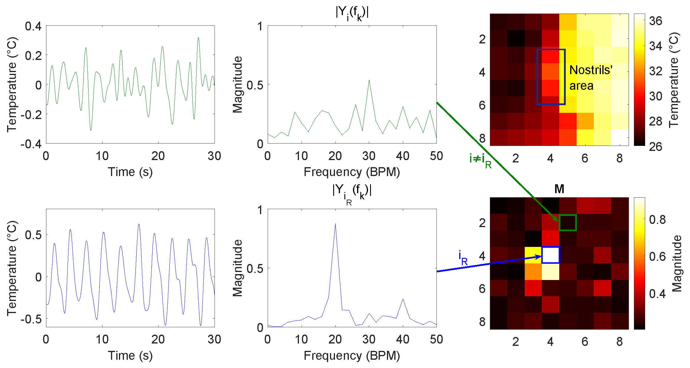
2.2.2. Pixel Selection and Pixel Update

The pixel containing the respiratory information should be identified. An approach was proposed in [20] where an empirical metric, SQI, was evaluated based on four features of the spectrum. The SQI is dependent, however, on empirically-chosen thresholds.

The method to identify the pixel with the strongest respiratory signal proposed in this work also operates in the Fourier domain. For each pixel, the time-domain samples were Hanning-windowed, then transformed through a 1D FFT, and the value of the highest peak in the normalized magnitude spectrum was used as a strength indicator. Consequently, an $8\times 8$ array of strength indicators was obtained, and the maximum element in this array was used to identify the pixel containing the respiratory signal.

Formally: let $x_i\left(n{T}_s\right)$ be the filtered, Hanning-windowed time-domain signal for the j^th window where the spatial mean has been removed; i is an index running through all $8\times 8$ pixels in the array, i.e., from 1–64, and the index $n=0+(j-1),1+(j-1),\dots ,N+(j-1)$ depends on the current window j; the number of samples per window was $N=300$, and the sampling time was $T_s=0.1$ s. $Y_i\left(f_k\right)$ is the spectrum of the i^th pre-processed time-domain signal $x_i\left(n{T}_s\right)$ and $\mid Y_i\left(f_k\right)\mid$ its magnitude, with $f_k=\frac{k}{N{T}_s}$ Hz and $k=0,1,\dots ,\frac{N}{2}-1$. We define the height of the normalized spectrum’s peak as:

$$m_i=\frac{{\displaystyle \underset{f_{min}\le f_k\le f_{max}}{max}}(\mid Y_i\left(f_k\right)\mid )}{\sqrt{{\displaystyle \sum _{f_k=f_{min}}^{f_{max}}}\mid Y_i\left(f_k\right){\mid }^2}},$$

(1)

where $f_{min}=0.167$ Hz and $f_{max}=0.667$ Hz, i.e., boundaries of the respiration band.

We assumed the respiration signal to be pseudo-periodic; thus, the spectrum would contain a peak. Noise, on the other hand, would show a relatively flat spectrum, as illustrated in Figure 2. In our algorithm, we interpreted a higher peak in the normalized spectrum as an increased likelihood that the pixel would contain the respiratory signal, and we only used a single pixel in the array, identified with index $i_R$ defined as:

$$i_R=\underset{i}{arg\; max}\left(\mathbf{M}\right),$$

(2)

where $\mathbf{M}$ is defined as:

$$\mathbf{M}=[m_1{m}_2\dots m_{64}].$$

(3)

The pixel needed to be selected for each window j. For the first w windows, the position was chosen by selecting the pixel with the highest peak in the normalized spectrum. The successive positions were, instead, dependent on the preceding w positions, limiting the search space of the following pixels. This procedure was intended to prevent rapid pixel-switching, which could deteriorate the computed spectra, whereas the scenario (substantially static subject) did not require rapid adaptation. A mask was created based on the w preceding positions that allowed the following ones to move only to an adjacent position. The value w was fixed empirically to 10.

2.2.3. Respiration Signal Extraction and RR Estimation

Once the pixel is selected, the respiration signal is obtained for each window as:

$$R\left(n{T}_s\right)=x_{i_{R_j}}\left(n{T}_s\right),$$

(4)

where $i_{R_j}$ indicates the pixel selected with the proposed method in the j^th window.

To estimate the RR, the Spectral Density (SD) needs to be calculated. SD can be estimated as the squared magnitude of the Fourier spectrum, known as the periodogram method:

$$P_{PER}\left(f_k\right)=Y_i\left(f_k\right)·Y_i{\left(f_k\right)}^{*}=\mid Y_i\left(f_k\right){\mid }^2.$$

(5)

Several other methods have been developed to estimate a more precise SD; Autoregressive (AR) models have already been used to extract respiration from PPG and have shown good potential [28]. AR models are parametric methods for signal modeling and SD estimation. The model assumes that a signal can be modeled based on the weighted sum of p precedent values. In the spectral domain, in particular, the SD can be estimated as the frequency response of a digital filter:

$$P_{AR}\left(f_q\right)=\frac{{\sigma }^2{T}_s}{{\left|1+{\displaystyle \sum _{b=1}^p}{a}_{b}exp(-j2\pi f_{q}b{T}_s)\right|}^2},$$

(6)

where ${\sigma }^2$ is the variance of the noise, $a_b$ are the weights of the AR model, and p is the model order. The weights need to be estimated and the order indicated. Moreover, it should be noted that this parametric model allows the estimation of $P_{AR}$ in an arbitrary number of points between 0 and $\frac{1}{2T_s}$; therefore, in general, $f_q$ can be different from the previously-defined $f_k$.

AR models are not directly affected by the Discrete Fourier Transform (DFT) limitations because they estimate the frequency response directly without implicit windowing and without spectral resolution restrictions. Therefore, AR models have been used especially when spectra need to be estimated on short windows. This parametric method is suited for narrowband signals with medium or high SNRs [29].

Several methods are available for autoregressive modeling; detailed information can be found in [30]. In this study, Burg’s method was chosen for its stability and accuracy on short data recordings. The model order p is not known a priori, and since there is no optimal method yet, many methods have been proposed in the years to correctly estimate it [31].

Chaichulee et al. [32] recently proposed to determine the order by choosing the p that minimizes the error obtained by comparing the peak of AR’s SD and the Fourier spectrum.

In this study, Chaichulee’s method has been used; the optimal model order was selected for each window, and $f_q$ was chosen to be equal to $f_k$. In Dataset B, the RRs have been estimated with both the AR model and periodogram, to compare the performances. The range of order was empirically chosen and went from 15–30 with a step of 1; whereas, in Dataset A, the periodogram method was used.

The RR was estimated as the frequency corresponding to the maximum magnitude. Once the RR were estimated, a moving median filter was applied averaging 10 estimations together and allowing us to obtain a new estimation of RR every second. Moreover, the time domain signal was reconstructed by gluing together the segments, as explained in [33].

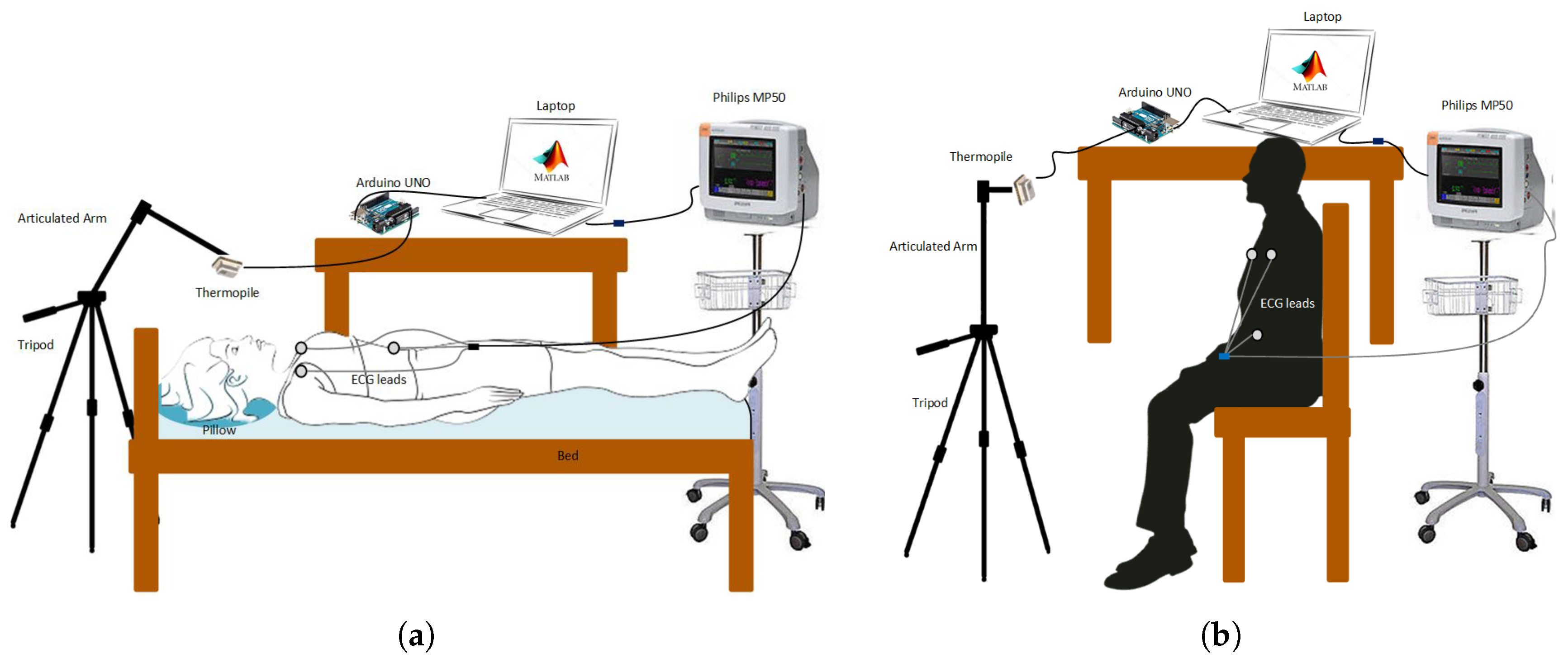
2.3. Experimental Setup

Thermal images were collected using a Grid–EYE thermopile array AM8854 from Panasonic. The sensor has 64 thermopile elements arranged in an $8\times 8$ grid, and it is sensitive in the Long Wave Infrared (LWIR) range. The field of view covered by the Grid–EYE is ${60}^{°}$, and it has a frame rate of $10$ Hz. The sensor was connected to an Arduino UNO through the I${}^{2}C$ bus, and the acquisition was performed through MATLAB.

The data collection was performed in a room with an ambient temperature of around 20 °C. It should be specified that respiratory activity causes also motion of the head and shoulders. This kind of motion is visible also in thermal images. Therefore, measurements to prove feasibility in flow detection have been taken with a subject lying down and shoulders out of the field of view. Moreover, measurements in seated positions have also been collected to prove the detection of respiration based on motion. Figure 3 shows the experimental setups. An impedance pneumography signal was used as the ground truth for respiration monitoring. Since the measurements were acquired in a stationary condition, the impedance pneumography signal can be considered reliable. The signal has been acquired using three ECG electrodes, as is common in clinical practice, and a patient monitor (Philips MP50) with a sampling frequency of $62.5$ Hz.

2.4. Datasets

The signals were collected in different orientations, at different distances, and with different breathing patterns. The subjects were asked to lay down as still as possible on a bed or sit on a chair and to breathe spontaneously or according to an audio stimulus. Two different datasets were collected: the first one to prove the detection of respiration with such a sensor in different settings, and the second one to prove the feasibility in the detection of respiration flow and to assess the performances of the proposed algorithm. Each signal had a duration of 2 min, resulting, after interpolation, in a matrix of $8\times 8\times 1200$. The study was approved by the Internal Committee Biomedical Experiments of Philips Research with ID: ICBE-2-26849, and informed consent has been obtained for each subject.

2.4.1. Dataset A: Constant Guided Breathing in Different Settings

The signals were collected on a single subject, since the purpose of the analysis performed was not to highlight inter-subject variability. For each condition, 3 signals were collected. Unless specified otherwise, the signals were collected during nasal respiration and with the subject lying down.

• Distance: signals were collected in side view with different distances, i.e., from 10–50 cm, and with constant RR of 20 BPM.
• Respiration rate: different RRs were used as the breathing pattern, i.e., from 10–30 BPM; signals were collected in side view with a constant distance of 20 cm.
• Orientation and oral/nasal respiration: the signals with constant RR of 20 BPM and distance of 20 cm were collected in side and frontal orientations during both nasal and oral breathing.
• Shoulder motion: the signals were collected in a seated position, with a constant RR of 20 BPM and a variable distance, i.e., 50 and 100 cm.

Overall, Dataset A consisted of 39 videos.

2.4.2. Dataset B: Guided Breathing with Different Patterns

Since this study is a proof-of-concept, we chose to use 5 subjects similar to the number of subjects used in [10] for their proof-of-concept study. Signals were collected with guided and spontaneous breathing. For each subject, two signals at constant RR of 10 and 30 BPM were collected, a signal with a linearly-variable RR, and a signal with an RR with two sudden change from 10–30 BPM. Moreover, signals during spontaneous respiration were collected. All the signals were collected in side view during nasal respiration at a distance of 20 cm. Overall, Dataset B consisted of 25 videos.

2.5. Evaluation

The signal to Noise Ratio (SNR), Root Mean Squared Error (RMSE), and Relative Error (RE) have been used to evaluate the accuracy of the thermopile in detecting the respiration signal.

SNR was evaluated according to:

$$SNR=10lo{g}_{10}\left(\frac{{\displaystyle \sum _{f_k=0.12}^{1.67}}\left(U\left(f_k\right)P\left(f_k\right)\right)}{{\displaystyle \sum _{f_k=0.12}^{1.67}}\left(\left(1-U\left(f_k\right)\right)P\left(f_k\right)\right)}\right),$$

(7)

where $P\left(f_k\right)$ is the signal’s spectral density estimated with the periodogram or AR method and $U\left(f_k\right)$ is a binary template window centered on the signal peak and first harmonic with a predefined width equal to 2 frequency bins. The first harmonic was included as the respiration signal is not a perfect sinusoid. The SNR was evaluated on each window, and the average of all the windows was used.

RMSE has been evaluated using the impedance pneumography as the reference:

$$RMSE=\sqrt{\frac{{\displaystyle \sum _{j=1}^L}{\left(\widetilde{RR}\left(j\right)-R{R}_{\mathit{ref}}\left(j\right)\right)}^2}{L}},$$

(8)

where $\widetilde{RR}$ is the respiration rate estimated, $R{R}_{\mathit{ref}}$ is the one detected by the impedance pneumography, and L is the number of windows evaluated. RE has also been estimated to allow a better comparison.

Moreover, signals collected in Dataset A have also been compared by assessing the number of pixels involved in the respiration signal. This was performed by evaluating the absolute value of the correlation coefficient between the detected respiration signal and the signals contained in other pixels. If the correlation was higher than 0.7, then the pixel was considered to contain respiration signal as well and was added to the pixel count.

The temperature variation detected by the thermopile due to respiration was also considered; this was obtained by using the range of the signal, i.e., the maximum amplitude minus the minimum amplitude. Both amplitude and the number of pixels have been estimated on each window and then averaged for the entire measurement.

3. Results

3.1. Dataset A

An overview of the analysis performed on Dataset A is shown in Figure 4; multiple distances, RRs, and frontal or side nasal/oral breathing have been compared. The dots and squares represent the means on the three signals collected for each setting, whereas the error bars show the standard deviations. Signals at distances of 20 and 30 cm, and 40 and 50 cm were grouped together, as a variation of 10 cm was not considered enough to show the effect of increasing distances. Therefore, in the distance case, the average and standard deviation were evaluated on six signals per setting. Moreover, Figure 5 shows the pixels containing the respiration signal in the case of a measurement taken at 50 cm in side view with the subject lying down and 50 cm in the frontal seated position, as well as the results obtained when the respiration was detected through shoulder motion.

3.2. Dataset B

Table 1. Average of five subjects of the results obtained on Dataset B.

Breathing Pattern	Periodogram			AR
	RMSE (BPM)	RE (%)	SNR (dB)	RMSE (BPM)	RE (%)	SNR (dB)
10 BPM	0.00	0.00	8.71	0.00	0.00	13.59
30 BPM	0.00	0.00	5.15	0.00	0.00	8.15
Chirp	1.41	1.19	4.09	1.41	1.21	5.87
Sudden Change	5.57	7.79	2.19	6.57	9.61	7.90
Spontaneous	0.98	1.59	4.27	0.99	1.72	5.81
Average	1.59	2.11	4.88	1.79	2.51	8.26

contains the average of the results obtained for each subject for the four different respiration patterns used, with both the periodogram and AR model. The last row shows the overall average results, in bold we indicate the best results for RMSE, RE, and SNR. Figure 6, instead, shows the time domain signals, the spectra evaluated through FFT on each window, and the RRs estimated in comparison with the reference for the five cases. It should be specified that in the case of guided breathing with a sudden change, an additional filter was applied. As can be expected from the results obtained in Dataset A, breathing at 30 BPM will have a lower amplitude compared to the 10-BPM one. This effect caused a delay in the detection of the frequency change. Therefore, a ramp filter has been applied to each window of the sudden change signals to amplify high frequencies in the breathing range. Correlation plots and Bland–Altman analysis for all the subjects and breathing scenarios are displayed in Figure 7. The mean bias was 0.23 BPM with the $95\%$ limits of agreement being $-5.05$–$5.51$ BPM. Moreover, the results also showed a strong correlation between the impedance pneumography estimated RR and the one estimated with the thermopile array, yielding an $r=0.95(p<0.0001)$.

4. Discussion

4.1. Dataset A

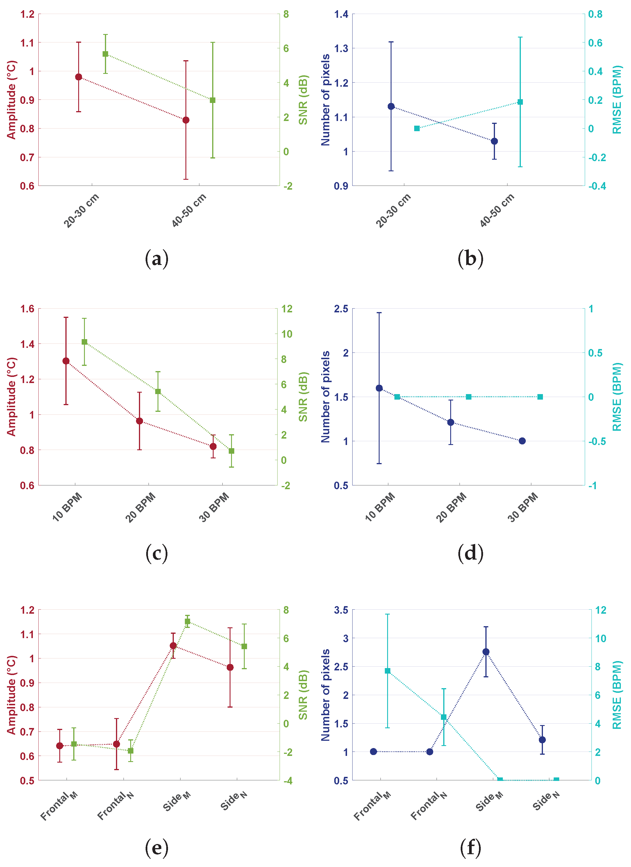
• Distance: Comparison of the performance between different distances proved that the thermopile would lose accuracy at larger distances. In particular, amplitude, SNR, and the number of pixels would decrease with larger distances, and the RMSE would increase. Amplitude decreased from an average of 0.98 °C to 0.83 °C. The SNR reduced from $5.66$ dB to $2.97$ dB, whereas RMSE went from $0$ BPM to $0.18$ BPM with a standard deviation of $0.45$ BPM. The number of pixels did not result in a big change on average, but it can be noticed that the standard deviation for the 20–30 cm case was much higher compared to the 40–50 cm case. This behavior was mainly due to the partial area effect. As already expected, the low resolution combined with the broad field of view limited the distance at which the sensor could be used.
• Increasing RR: Breathing with higher RR resulted also in a reduction of the amplitude from 1.30 °C to 0.82 °C, and the SNR drastically reduced from $9.34$ to $0.71$ dB, while the number of pixels from $1.60$ to $1.00$. The RMSE remained constant. These variations can be considered to be caused by the reduced flow during higher RR. The flow applied to the surroundings would be imposed for less time, due to the higher frequencies, reducing the heat exchanged.
• Orientation and oral/nasal respiration: In this dataset, both orientation and nasal/oral respiration were compared. Frontal measurements were expected to produce a reduced variation in temperature due to the small surface for heat exchanges available. Frontal nasal respiration resulted in performing particularly worse compared to the other settings. That is because the heat would be exchanged mostly with the nasal area around the nostrils. Frontal oral respiration performed better compared to the nasal case, but the RMSE was still much higher compared to the side cases. The improved performance in the frontal oral breathing could be due to the increased surface for heat exchanges, i.e., nose and lower lip, and to the higher temperature of oral expired air. Side oral respiration resulted in causing a bigger temperature variation and higher SNRs. This behavior was expected since in the side case, the pillow’s textile material would be involved in heat exchanges as well, increasing the surface. This setting involved many more pixels, i.e., on average $2.76$ compared to side nasal breathing, which resulted in $1.21$ pixels on average; whereas, the variation in amplitude and SNR was not as big. The differences can be explained by considering the differences in expired air temperature as already indicated in Section 2.1 and differences in the flow direction.
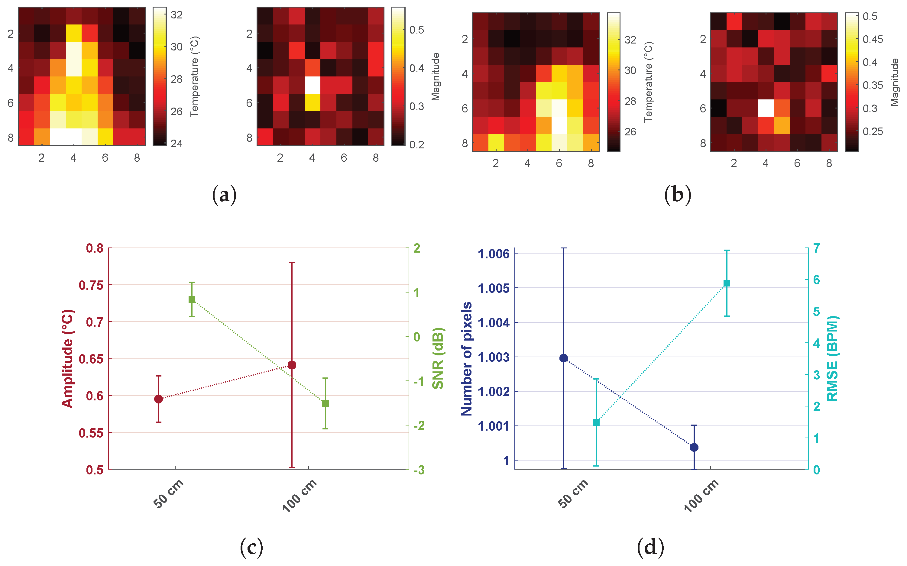
• Shoulder motion: Measurements were collected in a seated position at 50 and 100 cm when the shoulders were included in the field of view. Figure 5a,b shows the two different situations: in the first case, the signal resulting in the maximum peak magnitude was coming from the shoulder area, whereas in the second case (side view with the subject laying down), the signal was coming from the nose area. This was due to the fact that the temperature variation due to respiratory shoulder motion had a higher amplitude compared to the variation due to the heat exchanged because of respiratory flow in the frontal view at the same distance. Shoulder and head motion due to respiration can be suppressed by performing the measurement with the subject lying down. Moreover, due to the partial area effect of the sensor, the error in the detection of respiration through motion increased drastically already at 100 cm.

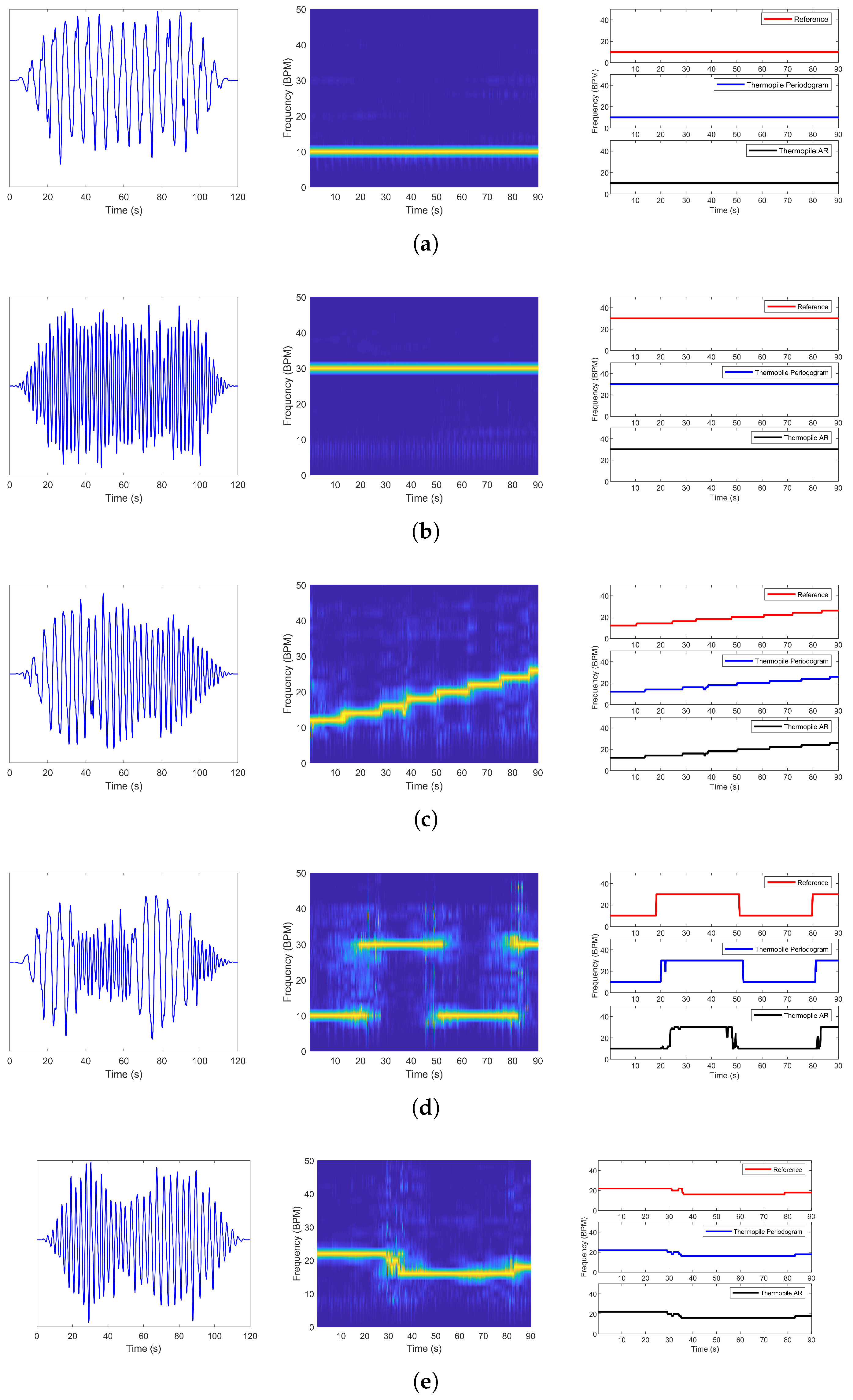
4.2. Dataset B

Constant breathing rates of 10 and 30 BPM both performed extremely well, resulting in an RMSE of $0$ BPM for both the periodogram and AR model; a difference in the SNR can be noted between the two RRs since the respiration at 30 BPM resulted in a lower SNR compared to the other one. This was already expected considering the results obtained in Dataset A. Chirp had a median error of $1.41$ BPM for the periodogram and $1.41$ BPM for the AR model, whereas the pattern with sudden change resulted in the highest RMSE, $5.57$ BPM and $6.57$ BPM, respectively. This was expected since in the sudden change case when indecision between the two peaks was present (similar height of the peaks in FFT), an error of 20 BPM could be obtained. Moreover, the sudden change was the only case in which the AR performed particularly worse compared to the periodogram. This can be explained considering that the SNR in this case was significantly lower compared to the other four cases, and AR is known to perform well in cases of high or medium SNRs. In the spontaneous breathing case, the RMSE resulted in being around $0.98$ for both SD estimators. Moreover, both correlation and Bland–Altman plots in Figure 7 show a bias in the estimated RR at 10 and $30$ BPM. This bias was due to a delay in the detection of the transition between 10 and $30$ BPM in the signals acquired with the sudden change pattern.

The periodogram yielded an average RMSE of $1.56$ BPM compared to $1.79$ BPM of the AR model; the RE was $2.11\%$ and $2.51\%$, respectively; and the SNR resulted in being on average $4.88$ dB and $8.26$ dB, respectively. The difference in error was on average only $0.23$ BPM, which we considered insignificant; whereas, the SNR was always higher in the AR model case. The similarity in the results is justifiable considering that Chaichulee’s method binds AR and Fourier spectrum evaluated through FFT to have the same RR estimation, therefore limiting AR models to the same limitations of DFT. Autoregressive modeling can improve the results obtained in short windows, but a new method for order selection should be investigated.

In this article, respiration detection using a thermopile array was proven to be feasible in a controlled environment and settings. It should be noted that this work is a proof-of-concept; future research should focus on proving the usability of such a sensor with a higher number of subjects and in clinical practice. Some limitations can be identified in the current approach, such as a lack of motion robustness and the pseudo-periodicity assumption for the respiration signal. Strategies to compensate motion are required. Considering that RGB cameras can currently monitor multiple vital signs and would be probably included in clinical practice in the future, a combination of RGB videos and thermopile array images could be used to track the identified pixel. A similar approach has been proposed in [11]; however, their solution relied on facial landmark detection; whereas, the pseudo-periodicity assumption would not hold in cases of apneas or other respiratory patterns. Strategies to overcome this challenge are definitely required before moving to clinical practice.

5. Conclusions

A thermopile array has been tested to prove the feasibility of respiratory flow detection. The results showed that respiration motion dominates the measurement for a seated subject. This indicates that a lying subject is crucial to measure respiratory flow successfully, rather than head and shoulder motion due to respiration. Moreover, the sensor has been proven to allow respiratory flow detection over a range of parameter settings, and with variable respiration rates. The pixel selection method successfully detected the pixel containing the respiration flow thermal signature.

The overall conclusion is that a thermopile array can be used for unobtrusive continuous respiration monitoring, and further development can provide interesting low-cost alternatives to the earlier microbolometer-based proposals.

References

1. Fieselmann, J.F.; Hendryx, M.S.; Helms, C.M.; Wakefield, D.S. Respiratory rate predicts cardiopulmonary arrest for internal medicine inpatients. J. Gen. Intern. Med. 1993, 8, 354–360. [Google Scholar] [CrossRef] [PubMed]
2. AL-Khalidi, F.Q.; Saatchi, R.; Burke, D.; Elphick, H.; Tan, S. Respiration rate monitoring methods: A review. Pediatr. Pulmonol. 2011, 46, 523–529. [Google Scholar] [CrossRef] [PubMed] [Green Version]
3. Pereira, C.B.; Yu, X.; Czaplik, M.; Rossaint, R.; Blazek, V.; Leonhardt, S. Remote monitoring of breathing dynamics using infrared thermography. Biomed. Opt. Express 2015, 6, 4378–4394. [Google Scholar] [CrossRef] [PubMed]
4. Di Fiore, J.M. Neonatal cardiorespiratory monitoring techniques. Semin. Neonatol. 2004, 9, 195–203. [Google Scholar] [CrossRef] [PubMed]
5. Fei, J.; Pavlidis, I. Virtual thermistor. In Proceedings of the 2007 29th Annual International Conference of the IEEE Engineering in Medicine and Biology Society, Lyon, France, 22–23 August 2007; pp. 250–253. [Google Scholar]
6. Lewis, G.F.; Gatto, R.G.; Porges, S.W. A novel method for extracting respiration rate and relative tidal volume from infrared thermography. Psychophysiology 2011, 48, 877–887. [Google Scholar] [CrossRef] [PubMed] [Green Version]
7. Murthy, J.N.; van Jaarsveld, J.; Fei, J.; Pavlidis, I.; Harrykissoon, R.I.; Lucke, J.F.; Faiz, S.; Castriotta, R.J. Thermal infrared imaging: A novel method to monitor airflow during polysomnography. Sleep 2009, 32, 1521–1527. [Google Scholar] [CrossRef]
8. Fei, J.; Pavlidis, I. Thermistor at a distance: Unobtrusive measurement of breathing. IEEE Trans. Biomed. Eng. 2010, 57, 988–998. [Google Scholar]
9. Abbas, A.K.; Heimann, K.; Jergus, K.; Orlikowsky, T.; Leonhardt, S. Neonatal non-contact respiratory monitoring based on real-time infrared thermography. Biomed. Eng. Online 2011, 10, 93. [Google Scholar] [CrossRef]
10. Cho, Y.; Julier, S.J.; Marquardt, N.; Bianchi-Berthouze, N. Robust tracking of respiratory rate in high-dynamic range scenes using mobile thermal imaging. Biomed. Opt. Express 2017, 8, 4480–4503. [Google Scholar] [CrossRef] [PubMed] [Green Version]
11. Scebba, G.; Tüshaus, L.; Karlen, W. Multispectral camera fusion increases robustness of ROI detection for biosignal estimation with nearables in real-world scenarios. In Proceedings of the 2018 40th Annual International Conference of the IEEE Engineering in Medicine and Biology Society (EMBC), Honolulu, HI, USA, 18–21 July 2018; pp. 5672–5675. [Google Scholar]
12. Fraden, J. Handbook of Modern Sensors: Physics, Designs, and Applications; Springer Science & Business Media: New York, NY, USA, 2004. [Google Scholar]
13. Mariani, G.; Kenyon, M. Room-temperature remote sensing: Far-infrared imaging based on thermopile technology. In Proceedings of the 2015 40th International Conference on Infrared, Millimeter, and Terahertz Waves (IRMMW–THz), Hong Kong, China, 23–28 August 2015; pp. 1–2. [Google Scholar]
14. Chen, W.H.; Ma, H.P. A fall detection system based on infrared array sensors with tracking capability for the elderly at home. In Proceedings of the 2015 17th International Conference on E-Health Networking, Application & Services (HealthCom), Boston, MA, USA, 14–17 October 2015; pp. 428–434. [Google Scholar]
15. Tanaka, J.; Shiozaki, M.; Aita, F.; Seki, T.; Oba, M. Thermopile infrared array sensor for human detector application. In Proceedings of the 2014 IEEE 27th International Conference on Micro Electro Mechanical Systems (MEMS), San Francisco, CA, USA, 26–30 January 2014; pp. 1213–1216. [Google Scholar]
16. Deckers, N.; Yildirim, M.; Reulke, R. Sensor Fusion-Based Learning for the Improvement of Person Segmentation by Means of a Low-Resolution Thermal Infrared Array Sensor. In Proceedings of the 2017 International Conference on Computer Graphics and Digital Image Processing, Prague, Czech Republic, 2–4 July 2017; p. 9. [Google Scholar]
17. Shetty, A.D.; Shubha, B.; Suryanarayana, K. Detection and tracking of a human using the infrared thermopile array sensor—“Grid-EYE”. In Proceedings of the 2017 International Conference on Intelligent Computing, Instrumentation and Control Technologies (ICICICT), Kannur, India, 6–7 July 2017; pp. 1490–1495. [Google Scholar]
18. Sun, G.; Saga, T.; Shimizu, T.; Hakozaki, Y.; Matsui, T. Fever screening of seasonal influenza patients using a cost-effective thermopile array with small pixels for close-range thermometry. Int. J. Infect. Dis. 2014, 25, 56–58. [Google Scholar] [CrossRef] [Green Version]
19. Lee, F.F.; Chen, F.; Liu, J. Infrared thermal imaging system on a mobile phone. Sensors 2015, 15, 10166–10179. [Google Scholar] [CrossRef] [PubMed]
20. Pereira, C.B.; Yu, X.; Goos, T.; Reiss, I.; Orlikowsky, T.; Heimann, K.; Venema, B.; Blazek, V.; Leonhardt, S.; Teichmann, D. Noncontact Monitoring of Respiratory Rate in Newborn Infants Using Thermal Imaging. IEEE Trans. Biomed. Eng. 2018, 66, 1105–1114. [Google Scholar] [CrossRef] [PubMed]
21. Pereira, C.B.; Yu, X.; Czaplik, M.; Blazek, V.; Venema, B.; Leonhardt, S. Estimation of breathing rate in thermal imaging videos: a pilot study on healthy human subjects. J. Clin. Monit. Comput. 2017, 31, 1241–1254. [Google Scholar] [CrossRef] [PubMed]
22. Gade, R.; Moeslund, T.B. Thermal cameras and applications: A survey. Mach. Vis. Appl. 2014, 25, 245–262. [Google Scholar] [CrossRef]
23. Abbas, A.K.; Heiman, K.; Orlikowsky, T.; Leonhardt, S. Non-contact respiratory monitoring based on real-time IR–thermography. In Proceedings of the World Congress on Medical Physics and Biomedical Engineering, Munich, Germany, 7–12 September 2009; Springer: Berlin, Germany; pp. 1306–1309. [Google Scholar]
24. Troost, M. Presence Detection and Activity Recognition Using Low-Resolution Passive IR Sensors. Master’s Thesis, Technische Universiteit Eindhoven, Eindhoven, The Netherlands, 3 April 2013. [Google Scholar]
25. Höppe, P. Temperatures of expired air under varying climatic conditions. Int. J. Biometeorol. 1981, 25, 127–132. [Google Scholar] [CrossRef] [PubMed]
26. Smith, I.; Mackay, J.; Fahrid, N.; Krucheck, D. Respiratory rate measurement: A comparison of methods. Br. J. Healthc. Assist. 2011, 5, 18–23. [Google Scholar] [CrossRef]
27. van Gastel, M.; Stuijk, S.; de Haan, G. Robust respiration detection from remote photoplethysmography. Biomed. Opt. Express 2016, 7, 4941–4957. [Google Scholar] [CrossRef] [PubMed] [Green Version]
28. Fleming, S.G.; Tarassenko, L. A comparison of signal processing techniques for the extraction of breathing rate from the photoplethysmogram. Int. J. Biol. Med. Sci. 2007, 2, 232–236. [Google Scholar]
29. Pardey, J.; Roberts, S.; Tarassenko, L. A review of parametric modelling techniques for EEG analysis. Med. Eng. Phys. 1996, 18, 2–11. [Google Scholar] [CrossRef]
30. Salinet, J.L.; Masca, N.; Stafford, P.J.; Ng, G.A.; Schlindwein, F.S. Three-dimensional dominant frequency mapping using autoregressive spectral analysis of atrial electrograms of patients in persistent atrial fibrillation. Biomed. Eng. Online 2016, 15, 28. [Google Scholar] [CrossRef] [Green Version]
31. Aydin, S. Determination of autoregressive model orders for seizure detection. Turk. J. Electr. Eng. Comput. Sci. 2010, 18, 23–30. [Google Scholar]
32. Chaichulee, S.; Villarroel, M.; Jorge, J.; Arteta, C.; Green, G.; McCormick, K.; Zisserman, A.; Tarassenko, L. Localised photoplethysmography imaging for heart rate estimation of pre-term infants in the clinic. In Proceedings of the Optical Diagnostics and Sensing XVIII: Toward Point-of-Care Diagnostics. International Society for Optics and Photonics, San Francisco, CA, USA, 29–30 January 2018; Volume 10501, p. 105010R. [Google Scholar]
33. De Haan, G.; Jeanne, V. Robust pulse rate from chrominance-based rPPG. IEEE Trans. Biomed. Eng. 2013, 60, 2878–2886. [Google Scholar] [CrossRef] [PubMed]
Figure 1. Block diagram summarizing the processing chain from images’ acquisition to respiration rate extraction.
Applsci 09 02449 g001
Figure 2. The upper plots show the time domain signal and spectrum of a pixel where no respiratory information is present. The plots on the second row show the time domain and spectrum of another pixel that contains a respiration signal; whereas, the upper figure shows a thermal image where a subject is in a profile view at 20 cm from the sensor, the lower one showing the distribution of the normalized spectrum’s peak calculated per each pixel, i.e., M resulting from Equation (3). The pixels containing the signals plotted are indicated. BPM, Breaths Per Minute.
Applsci 09 02449 g002
Figure 3. Experimental setup: (a) subject lying down on a bed; (b) subject in a seated position.
Applsci 09 02449 g003
Figure 4. Overview of the differences in amplitude, SNR, number of pixels, and RMSE in Dataset A: (a,b) results for signals acquired at different distances; (c,d) comparison of different Respiration Rates (RRs); (e,f) different orientations and oral and nasal respiration; M and N indicate respectively mouth and nose breathing.
Applsci 09 02449 g004
Figure 5. Respiration detection through shoulder motion: (a,b) the first figure shows a thermal image, and the second one shows the spectrum peak magnitude distribution of a subject seated and lying respectively at 50 cm of distance; (c,d) overview of the differences in amplitude, SNR, number of pixels, and RMSE when data were collected from a seated subject at 50 and 100 cm.
Applsci 09 02449 g005
Figure 6. Results obtained for Dataset B with different patterns; on the left the time domain signal, in the middle the Fourier spectrum per each window, and on the right the RR extracted with both the periodogram and AR and the impedance pneumography one. (a,b) Collected during constant breathing pattern at 10 and 30 BPM, respectively; (c) chirp pattern; (d) pattern with two sudden changes; (e) spontaneous breathing. The time axis in the FFT and in the extracted RR figures ends at 90 s even though the original signal has a duration of 120 s. This is due to the sliding window approach using a window size of 30 s.
Applsci 09 02449 g006
Figure 7. Bland–Altman plot and correlation plot for all the subjects and settings in Dataset B. Reference indicates the RR estimated with the impedance pneumography, whereas estimate indicates the one estimated using the thermopile array. In the Bland–Altman plot, the blue horizontal line represents the mean bias, whereas the two horizontal black lines indicate the average plus or minus 1.96 · S t a n d a r d D e v i a t i o n . The black line in the correlation plot indicates the linear relationship y = x.
Applsci 09 02449 g007