Article

An Evaluation Framework to Support Optimisation of Scenarios for Energy Efficient Retrofitting of Buildings at the District Level

by
Miguel Á. García-Fuentes
1,*,
Víctor Serna
1,
Gema Hernández
1 and
Alberto Meiss
2
1
Energy Division, CARTIF Technology Centre, 47151 Boecillo, Spain
2
Dpto. de Construcciones Arquitectónicas, Universidad de Valladolid, 47014 Valladolid, Spain
*
Author to whom correspondence should be addressed.
Appl. Sci. 2019, 9(12), 2448; https://doi.org/10.3390/app9122448
Submission received: 14 April 2019 / Revised: 9 June 2019 / Accepted: 11 June 2019 / Published: 14 June 2019
(This article belongs to the Special Issue Smart Home and Energy Management Systems 2019)

Abstract

:

Featured Application

Design of energy-efficient retrofitting projects of buildings at the district scale.

Abstract

Energy-efficient retrofitting of buildings has become essential to achieve the environmental objectives of the European Union’s (EU) strategies towards reducing carbon emissions and energy dependency on fossil fuels. When tackling retrofitting projects, the issue of scale becomes essential as sometimes this can determine the sustainability of the project. Therefore, a comprehensive approach is essential to ensure effective decision-making. A platform has been designed within the EU funded OptEEmAL project to support stakeholders in this process, providing functionalities that can automatically model and evaluate candidate retrofitting alternatives considering their priorities, targets and boundary conditions. A core element of this platform is the evaluation framework deployed which implements a multi-criteria decision-making approach to transform the priorities of stakeholders into quantifiable weights used to compare the alternatives. As a result, more informed decisions can be made by the stakeholders through a comprehensive evaluation of the candidate retrofitting scenarios. This paper presents the approach followed to develop and integrate this evaluation framework within the platform as well as its validation in a controlled environment to ensure its effectiveness.

1. Introduction

As stated by the Energy 2020 strategy, the reduction of Greenhouse Gas (GHG) emissions in the European Union (EU) can only be achieved if tackling appropriate the big potential existing when increasing energy efficiency [1]. This is particularly relevant in the built environment, where high energy savings can be achieved [2].
However, there are still a number of challenges that need to be addressed due to the low effectiveness of existing practices, as they used to underexploit the interactions among buildings, trade-offs or synergies. Apart from the issue of considering the buildings as part of a more complex system, there is a challenge on evaluating the parameters related to energy efficiency or sustainability, which are usually too focused on a very specific aspect such as “energy consumption” and ignore other relevant parameters and impacts [3]. This evaluation, which is carried out through the use of simulation tools, results in different levels of accuracy but generally “imply the generation of ad hoc simulation models” [4]. This process is always prone to human error—not only when creating the simulation models, but also when incorporating energy conservation measures. Due to the complexity of the problem and as this process is tedious and consumes a lot of time, usually a reduced set of technologies is considered, “hindering the possibility to find an optimal retrofitting solution” [5].
Furthermore, the construction sector is slowly turning into a new paradigm of more collaborative approaches for the stakeholders, as building information modelling (BIM) [6] and integrated project delivery (IPD) [7] aiming at creating better mechanisms for information exchange and interaction and, on top of this, delivering more effective processes while reducing costs.
In this context, the objective of the platform developed is to offer a collaborative solution “for the energy-efficient retrofitting at district scale” [8], integrating the following elements to address the problems described above:
  • Assessment at district scale: the tool considers the interaction among buildings and analysis the potential existing when considering the district as a whole and analyses the inter-building interaction both in terms of passive and active relationships. This is done through the implementation of tools that can enrich the models through adding the shadows that affect the buildings under study [9] in order to perform an appropriate evaluation at district level. At the same time, technologies are proposed at district level, exploiting the synergies among buildings in terms of sharing energy systems and energy production [10].
  • Use of Multiple-Criteria Decision Analysis: the evaluation framework is based on evaluating the performance of the candidate scenarios against a set of criteria in different fields, offering a more comprehensive evaluation and more informed decision making.
  • Energy Conservation Measures (ECMs) catalogue: the tool provides a wide catalogue of existing technologies that can be implemented at different scales (zone, building, district) and different fields (passive, active, RES or control).
  • Use of standards: use of standard file formats for building definition (Industry Foundation Classes, IFC) [11], and district scale (CityGML) [12], to ensure the implementation of a collaborative approach and interoperability among the different components and tools.
  • Interoperability: the use of standards and the generation of a District Data Model ensure the interoperability among the tools that have been integrated for the processes of generating, evaluating and optimising the candidate retrofitting scenarios.
  • Use of Integrated Project Delivery (IPD): the tool fosters the implementation of more collaborative approaches as IPD towards ensuring more informed decisions and improved processes compared to business-as-usual [7].
Considering all these elements, the OptEEmAL tool provides four processes into an integrated solution around an interoperability framework to ensure appropriate use and exploitation of data. These processes are:
  • Data insertion (1). Users insert the required data into the tool to perform the evaluation of the baseline and to create the candidate retrofitting alternatives.
  • Data integration and baseline calculation (2). After the users have inserted the data, the OptEEmAL tool creates the first instance of the data model (baseline) and calculates the values of the relevant indicators to characterise its performance. For this, a set of simulation models are created and processed through simulation tools to retrieve and post-process these indicators which are calculated at district level.
  • Scenarios generation and optimisation process (3). Once the baseline is calculated, the tool generates a set of candidate retrofitting scenarios based on implementing Energy Conservation Measures to the baseline model. These models are then calculated through the simulation tools integrated into the tool and provide the indicators that characterise their performance. Groups of scenarios are generated and evaluated until the stopping criteria are met.
  • Outcomes exportation (4). After calculating the best scenarios, these are presented to the users of the tool who can select the most suitable and export all data that has been produced for it.
All these four processes together allow for delivering more informed decisions and reducing time and costs of the design process, having also an impact on the subsequent stages of the process. A core element in the design and development of the OptEEmAL tool is on the role and integration of the users and the way of transforming their subjective establishment of preferences into a mathematical problem to drive the optimisation of the retrofitting scenarios.
As stated above, one of the novelties of the tool presented is the fact that it tackles the design and optimisation problem at district scale, analysing therefore the inter-building effects. This is done in terms of three main processes: a) indicators are computed and aggregated at district level so that the optimisation allows balancing the district as a whole, b) to ensure that simulations are district-aware, the effects of surrounding district environment is considered, and c) energy systems at district scale are included as part of the catalogue so that it is ensured that the technologies proposed not only optimise the building performance, but also the district performance.
The calculation of indicators at the district scale is done by means of aggregation of indicators at lower levels (space, building, etc.) These are calculated with the tools integrated within the OptEEmAL platform and then post-processing and aggregation techniques are implemented to build the district performance indicators which are used for the optimisation approach presented within this paper.
With regards to computing and evaluating the inter-building effects, these occur mainly at passive and active level, corresponding with the assessment of the effect that the surroundings have within the evaluated buildings that form the district, and with the integration as candidate ECMs of technologies at district scale respectively. In order to ensure that the effects are appropriately modelled and then calculated, a district neighbour shading (DNS) tool has been deployed which uses an algorithm developed to determine the set of surfaces that block the solar energy from entering the simulated buildings [9]. This tool receives the information coming from the IFC and CityGML models and then, based on input variables as the latitude, longitude, and the identification of the buildings under study, it provides the geometry of the shading surfaces as a XML file [13]. This file is then used in order to enrich the original model through a set of geometry enrichment processes which not only include the addition of shadowing surfaces, but also other information as the second-level space boundaries [14] that allow populating some missing information within the original IFC file in order to provide to the simulation tools the appropriate information on the building polygonal surfaces through which the thermal energy is exchanged [15].
To ensure that the active inter-building effects are also considered, the catalogue developed within the tool to generate the candidate retrofitting scenarios contains measures structured at different levels, ranging from space to district level. The ECMs included at district level consider the thermal and electrical balancing of the district through integrating systems that produce energy locally and distributes it among the buildings of the district. The thermal measures proposed include basically district heating networks where two approaches are considered: either the retrofitting of existing networks or the implementation of new networks to cover the reduced thermal demand of the buildings (after the implementation of passive measures). For electrical consumption, the buildings with highest potential for integration in terms of geometry and orientation are considered to maximise the potential production.
This paper provides an overview of the platform developed (Section 2), and then focuses within the methodology followed in order to deploy the evaluation procedure that transforms users’ requirements to setup the optimisation problem (Section 3). Then, a simple case in a controlled environment to assess this evaluation procedure is depicted (Section 4), showing then the main results and conclusions (Section 5 and Section 6, respectively). It should be noted that a complete assessment of the tool is not the focus of this paper. The results shown here are the basis to assess the evaluation method to then scale-up the problem to wider complexities in terms of the considered geometries, building interactions and ECMs.

2. Platform Approach

As the following Figure 1 shows, there are five core processes that respond to the steps introduced above and with the overall aim of offering the functionalities required to support decision making when designing energy-efficient retrofitting projects.

2.1. Problem Definition

According to the description above, the process starts with the insertion of data required to define the baseline (IFCs, CityGML, contextual data, and other data related to the project) and with the definition of the objectives, barriers, targets or boundaries by the user so that the tool can design the retrofitting solution according to this information [17]. Furthermore, before launching the automatic generation of scenarios, simulation and optimisation, the list of the measures to be considered in the optimisation problem will be made available for the user to check and edit if necessary. Furthermore, targets and boundaries can be set by the users to make more precise the definition of scenarios. This information is inserted along with the prioritisation criteria as it is explained within the evaluation process showcased in this paper and detailed within the sections below.

2.2. Simulation and District Performance Indicators (DPI) Calculation for the Baseline

Simulation models of the baseline are then processed by a set of simulation tools that are used for the calculation of the 42 indicators that define the evaluation framework. Depending on the indicator that is calculated, a different tool is used: “energy DPIs are calculated with the results offered by the external simulation tools Energy Plus®” [18] and “HVAC and controls simulation tool developed within the platform” [19], while “environmental DPIs are determined with the help of NEST®” [20]. The combination of some of these indicators allows the calculation of others. Once the simulation models have been executed, the results are then aggregated resulting into the values of the 42 indicators at district level.

2.3. Scenarios Generation Through an ECMs Catalogue

After the generation and simulation of the baseline according to the process described above, the user is presented with the values of the baseline indicators and an iterative process of scenarios generation and optimisation is launched. Thus, different scenarios are created through the application of one or more ECMs from the catalogue to the baseline scenario.
These are mapped into the simulation model that represents the baseline, and then are executed with the set of simulation tools to calculate the indicators as it occurred for the simulation of the baseline. Thus, the simulation models for the scenarios are executed, and the DPIs for every candidate retrofitting scenario are stored within the platform.

2.4. Evaluation and Optimisation

The evaluation method deployed within the platform is aimed at translating the qualitative into quantitative which “is the research topic of multi-criteria decision analysis” (MCDA) [21,22]. Thus, MCDA can be used in order to create a framework for decision making when evaluating alternatives for designing a retrofitting solution analysing a set of evaluation criteria (in this case, indicators calculated at district level).
The use of a weighting method is the main procedure but although there some approaches as ISO standards [23], the aggregation method to be used is not defined. Furthermore, there are also a number of elements that need to be solved when implementing this sort of decision-making approaches [24]. Some of these challenges can be highlighted as, for example, defining the evaluation criteria, normalising and scaling the indicators or defining the objectives and weighting schemes.
The solution proposed by this evaluation methodology is the one reflected within Figure 2 above. This process considers first the normalisation of the evaluation criteria in order to make them comparable, then an aggregation method is implemented to calculate two functions: the one representing the cost, and the one reflecting the benefit, which allows ordering the scenarios and comparing them to select those most suitable to the targets defined by the user.
A harmony search optimisation algorithm allows repeating the generation of groups and scenarios and their evaluation in terms of the cost and benefit functions [25]. This algorithm generates new iterations in the form of groups of candidate retrofitting scenarios, which are created based on the results that are obtained from the previous execution and, therefore, optimising them in a continuous loop.

2.5. Finding the Best Results

The optimisation process occurs in a loop where new scenarios are generated and evaluated and it stops when the stopping criteria are met. These criteria are defined through the inputs provided by the users in terms of targets and boundaries to the optimisation problem.
Once this happens, the user is shown with a set of best scenarios represented in a Pareto front where the user can visualise the performance and ECMs applied in each of them, and then selecting and exporting the results of the one preferred.

3. Methodology: Development of the Evaluation Framework

An optimisation problem is defined as “the one aimed at finding the solutions that are optimal or near-optimal with respect to some goals and translated into an objective function” [26].
This function can be bi-objective (based on the optimisation of two indicators at the same time), or consider more dimensions being therefore a multi-criteria objective function. These two methods can also be combined, where DPIs can be grouped to represent composite indexes that can characterise the performance of the buildings or district to be retrofitted.
The selection of the method highly depends on how the decision maker is formulating the problem and on establishing properly the importance of the criteria that is used for the evaluation. Therefore, within this methodology, the objective function depends on the prioritisation scheme established to represent the importance of each DPI.

3.1. Evaluation Criteria Selection

The method deployed within this framework considers the principles of IPD (decision-maker definition) in order to enable the decision-making process, where the evaluation criteria are defined as DPIs. In overall, the platform considers 42 DPIs covering six relevant fields. However, in order to facilitate the comprehensive evaluation of the performance of a district the list to be used for the evaluation was reduced to 18 DPIs “after having analysed if they were natural or easily measured attributes, constructed attributes, which coalesce several natural attributes, or proxy attributes (evaluation criteria)”, as suggested in [27].
The indicators have been aggregated into one group that represents the benefits and another that represents the costs. Additionally, a third category has been created within the benefit group in order to ease the establishment of the prioritisation criteria, as explained in the following section. Thus, the evaluation criteria are divided into:
  • Cost Group: This group contains the DPIs that indicate the cost for the scenario (environmental or economic cost).
  • Benefit 1 Group: This group involves the DPIs that could show a benefit for the scenario (reduction of energy demand or consumption, increase of the energy demand covered by renewable sources, increase of comfort…).
  • Benefit 2 Group: This group takes into consideration the benefits obtained when increasing the contribution of renewable energies: photovoltaics, solar thermal, hydraulic, mini-eolic, geothermal and biomass. It is a sub-group of the Benefit 1 Group, since it represents a disaggregation of the indicator that measures the Energy demand covered by renewable sources (ENE09), where the energy demand covered by renewable sources can be further analysed.
Table 1 shows the DPIs included in each of these groups, where ENV corresponds to the environmental indicators, ECO to the economic aspects, ENE to those energy related and COM to those that represent the comfort performance of the district.
It should be noted that the numbering of the indicators is not correlative, as they are a selection from the list of 42 indicators used within the platform to characterise the performance of the district as mentioned above.

3.2. Definition of the Optimization Problem

Multi-objective optimization, also called multi-criteria optimization, can be defined as “the problem of finding a solution vector of decision variables which satisfies the project constraints introduced by the end users and optimizes a vector function whose elements represent individual objective functions” [28]. These functions form a mathematical description of performance criteria (DPIs). Hence, the term “optimise” means finding such a solution vector (refurbishment scenario) which would give the values of selected DPIs acceptable according to the predefined targets and boundaries.
Formally, a multi-objective optimization problem is defined so as to find the solution vector x = [x1, x2,…, xn] T which optimizes the district performance vector defined as:
D ( x ) = [ f 1 ( x ) , f 2 ( x ) , f n ( x ) ] T
In other words, the goal is to determine among the set of all feasible refurbishment scenarios that satisfies the constraints, the particular set x which yields the optimum values of the selected DPIs defined in equation f(x).
Note that in general there is not a single point optimizing the set of objective functions, whereas a set of optimal solutions considered being non-dominated solutions or Pareto set approximation. Therefore, the notion of “optimum” varies with respect to mono-objective approaches, which aims at achieving a unique solution that simultaneously meets the constraints and provides the best value for the objective function. In multi-objective approaches, a solution vector x is Pareto optimal if there does not exist another x, such that fi(x) ≤ fi(x) for all i > {1,…, n} and fj(x) < fj(x) for at least one j.
This definition means that x is Pareto optimal if no feasible vector of decision variables exist which would decrease some criterion without causing a simultaneous increase in at least another criterion. The plot of the objective functions whose non-dominated vectors are in the Pareto optimal set is called the Pareto front [29]. In the present approach and as depicted before, the evaluation criteria has been divided into three groups representing the costs the first, and the benefits the second and third (being this last one a subcategory of the second). Therefore, the optimization problem here is the one that aims at finding the set x that minimizes the costs (considering not only economic costs but also environmental or social costs) and maximizes the benefits, which are plotted in order to find those optimal contained in the Pareto front.
However, in order to find the cost and benefit values for each candidate retrofitting scenario, a weighted sum of the indicators that represent these two indexes has to be carried out, where the weights have to represent the prioritization criteria established by the stakeholders.

3.3. Building the Cost–Benefit Function

3.3.1. Establishing a Weighting Method

According to [27], weighting methods (in this case to solve energy efficient retrofitting design problems) can be considered into four main groups, which are: proxy approaches through selecting one or various indicators, monetisation methods in which environmental impacts are translated into monetary units, ‘distance-to-target’ or panel methods.
The evaluation framework implemented within this tool follows the panel method approach and it is implemented through two methods. In the first one the users are enabled to compare the importance of indicators by pairs so that they are not conditioned by their interpretation of the whole scheme and can perform a more accurate comparison. The second enables the user to select a pre-defined weighting scheme which has been developed and deployed within the tool by a group of experts implementing the pairwise comparison of indicators for a set of goals as priority to reduce the energy consumption, the GHG emissions or the optimisation of the operational costs.

3.3.2. Normalisation and Scaling

There exist many normalisation techniques and according to [30], “both robustness (insensitivity against the existence of extreme values) and efficiency (estimated value close to the expected optimum when the real data distribution is unknown) must be balanced”. Through the application of normalization, the values used to feed the evaluation matrix will turn into non-dimensional, taking all of them values in the interval [0,1], and where in all of them 0 represents the worst value for the indicator (the less sustainable) and 1 represents the best value (the most sustainable).
Normalisation is aimed at transforming current values for each criterion that is measured under different units, into a common new criterion that follows the same unit. According to [31], three different methods can be applied, being the most suitable to address a synthetic transformation of the value of the indicators following a fixed scale unit change. The normalisation and scaling method in this methodology intends to reduce the amount of subjectivity in the process by making use of the results derived from the calculation of the baseline scenario. Thus, instead of fixing the minimum and maximum values to implement a min-max normalisation, relative values compared to the baseline situation are used.
Then, since most DPIs measure the savings obtained in each category (for example “savings in energy consumption” measured from 0% to 100%) this can be easily related to the best possible obtainable value, which is a 100% of savings = “1”, while the worst value (“0”) would be a 0% of savings.
However, not all DPIs can be calculated as savings against the baseline situation (as, for example, the investment), using in these cases the values given by the stakeholders as boundary condition to transform the criteria into a homogeneous framework that can be weighted and aggregated.

3.3.3. Building a Panel Method Scheme: Analytic Hierarchy Process

Panel methods to elicit the criteria highly depend on the selected method (questionnaires, interviews, or group discussions), panel composition (experts, laypeople, or stakeholders), procedure (single-round, Delphi) and outcome (consensus, statistical analysis of results) [32]. In the case of this evaluation method, and according to the IPD principles, the panel will be composed by the stakeholders being articulated through the IPD contract, and must result into a consensus to elicit the weighting parameters.
There are several panel methods which can be implemented, being those more relevant: direct rating, Simos’ cards method, ranking the criteria, pair-wise comparison (for example in the analytic hierarchy process, AHP), and the classical multi-attribute value theory (MAVT). which may be adapted for other procedures [33].
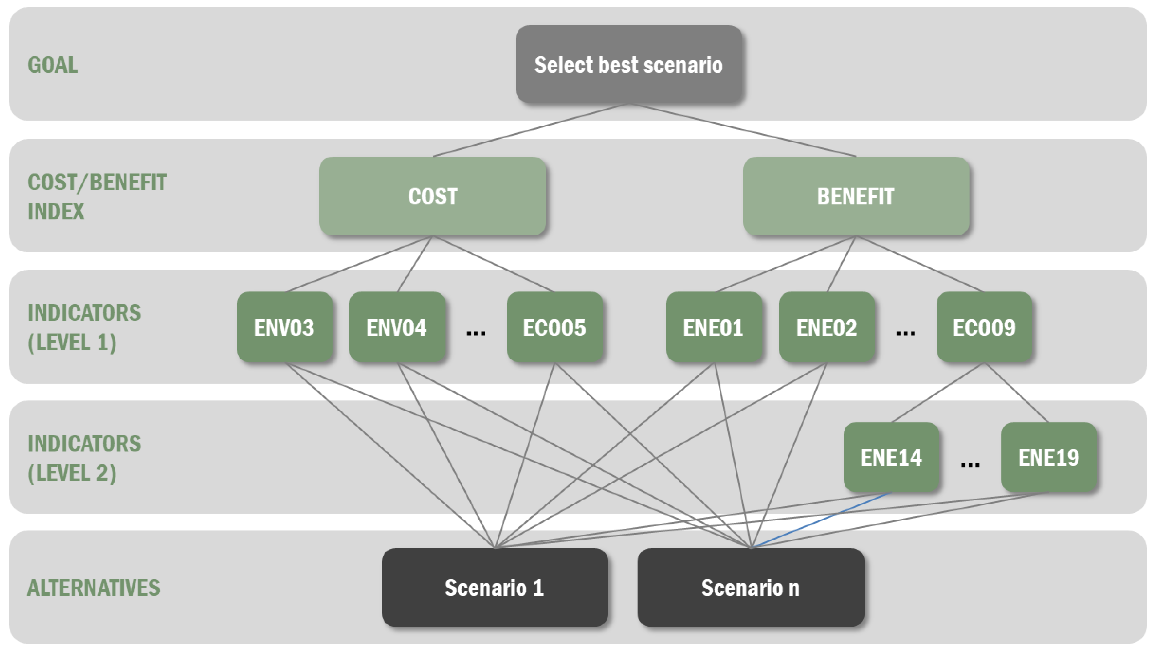
Below, the main scheme of an analytic hierarchy process (AHP) is presented in Figure 3, which establishes that [34]: “a decision making process can be decomposed into 4 steps, namely: defining the goal, structure the decision hierarchy, construct a set of pairwise comparison matrices and use the priorities obtained from the comparison to weight the priorities in the level immediately below”.
The AHP process is a well-known method that serves to establish the relevance for each criterion through their comparison per pair. As the state-of-the-art demonstrates, it is a consistent method that can be used in order to solve different decision making problems. In this case, the problem to be solved is the selection of the best scenario from the alternatives through considering the priorities of the stakeholders.
Thus, this tool proposes and integrates a pair-wise comparison strategy that allows generating a weighting scheme through comparing per pairs the main criteria with respect to the cost/benefit index and the sub-criteria (level 2 of indicators) with respect to the criteria ENE09.
The values related to the intensity of importance, according to [35], “have to be set by consensus of the decision making panel (or experts’ panel for fixed weighting schemes), in which each participant is asked individually to compare the criterion in a pairwise method setting whether a criterion is more important than the pair, and by how much”. Table 2 shows the scale of numbers used to reflect the intensity of importance of the indicators.
Following this approach, the process considers the construction of the pairwise comparison matrices that can establish the relevance of each criterion for a defined goal. In this evaluation method, there are three matrices that allow comparing:
  • Pairwise comparison matrix of the six environmental and economic criteria with respect to cost.
  • Pairwise comparison matrix of the six energy and comfort criteria with respect to the benefit.
  • Pairwise comparison matrix of the six criteria for the renewables with respect to ENE09.
In the following Table 3, Table 4 and Table 5, these three comparison matrices are shown.
According to AHP, this matrix is reciprocal, meaning that when comparing each criterion against itself the result is 1, while the comparisons on the right of the diagonal are the inverse of those located on the left of the diagonal.
After generating the matrices of comparison, “the weight of each indicator is calculated through solving the eigenvector, which is based on a three steps process” [36]:
  • The matrix has to be raised to powers squared successively each time.
  • The sum of the rows is calculated and then normalised.
  • Once the difference between the sums of two consecutive calculations is lower than a value that has been defined, then the calculation stops.
The values of the weight are the sum of the rows for this matrix.
This process allows obtaining the weights of each criterion and then building the cost and benefit functions. The following equation reflects the example of the cost group matrix:
[ w E N V 03 w E N V 04 w E N V 06 w E C O 02 w E C O 03 w E C O 05 ] = [ 1 E N V 01 E N V 04 E N V 01 E N V 06 E N V 01 E C O 02 E N V 01 E C O 03 E N V 01 E C O 05 E N V 04 E N V 01 1 E N V 04 E N V 06 E N V 04 E C O 02 E N V 04 E C O 03 E N V 04 E C O 05 E N V 06 E N V 01 E N V 06 E N V 04 1 E N V 06 E C O 02 E N V 06 E C O 03 E N V 06 E C O 05 E C O 02 E N V 01 E C O 02 E N V 04 E C O 02 E N V 06 1 E C O 02 E C O 03 E C O 02 E C O 05 E C O 03 E N V 01 E C O 03 E N V 04 E C O 03 E N V 06 E C O 03 E C O 02 1 E C O 03 E C O 05 E C O 05 E N V 01 E C O 05 E N V 04 E C O 05 E N V 06 E C O 05 E C O 02 E C O 05 E C O 03 1 ] 8 [ 1 1 1 1 1 1 ]

3.3.4. Cost–Benefit Function

As depicted above, the main objective therefore is to establish the cost–benefit functions D(x) to be optimized so that the set x can be found to minimize the cost and maximize the benefit, and where this set x is represented through the Pareto front.
The following Table 6 summarises the aggregation of the indicators following the approach depicted in the previous sections, in order to build this cost–benefit function:
Thus, the benefit (3) and cost (4) functions can be formulated in the following manner:
B ( x ) = i = 1 n w E N E i · I E N E i ( x ) + i = 1 n w C O M i · I C O M i ( x )
C ( x ) = i = 1 n w E C O i · I E C O i ( x ) + i = 1 n w E N V i · I E N V i ( x )
These functions represent the performance of the district for every candidate scenario and are those to be optimised in order to find the set of best scenarios according to the prioritisation criteria that has been inserted as weights to the indicators.

4. Case Study: Validation of the Evaluation Approach in a Controlled Environment

The evaluation method presented within this paper has been implemented within an evaluation tool that retrieves the input data required in order to perform the evaluation and provide the Pareto front in order to optimise the retrofitting scenarios.
As input data for the evaluation, the diagnosis DPI results, the evaluation DPI results (associated to each candidate retrofitting scenario), and the targets, boundaries and weights established by the stakeholders are required. As an outcome, the evaluator provides the cost and benefit functions and the lists of DPIs outside boundaries as well as the list of targets reached.
In order to test the evaluator and the evaluation methodology, a case study was carried out within a controlled environment to validate and assess the proposed method. Since it was an isolated validation, it is important to note the following aspects with regards to the case:
  • The ECMs selected to create the scenarios were obtained from the ECMs catalogue developed for the platform.
  • The scenarios considered were generated following the intelligence implemented in the scenario generator described at the beginning of this paper, considering the constraints established by the user.
  • The calculation of the baseline and scenario DPIs were retrieved following the normal and operational process of the platform (that is, with the evaluator integrated within it), and therefore queried to the corresponding repositories of the tool.
  • Also the weighting schemes, targets and barriers were obtained from the corresponding repositories, that is, the pre-defined weighting schemes were already available within them.

4.1. Description of the Case Study

The validation has been performed based on the results obtained in a simple case which has been created for this aim as shown in the table below (Table 7).
A total of 14 ECMs have been combined to create 178 scenarios that combine the measures. The measures selected are the following:
  • 4 types of external wall insulation with different thicknesses of insulation (50-100-150-200 mm)
  • 4 types of internal wall insulation with different thicknesses of insulation (40-60-80-100 mm)
  • 4 types of roof insulation with different thicknesses of insulation (40-60-80-100 mm)
  • Replacement of the existing energy system with the installation of a natural gas boiler
  • Installation of PV panels on roof
The logic followed to generate the 178 candidate retrofitting scenarios considered different combinations of the measures listed above. First each passive measure has been considered separately, and then to each separate passive measure an active or renewable measure has been added. Next, the combination of passive measures has been explored (external/internal insulation + roof), without considering the implementation at the same time of internal and external insulation to façades. To it also active and renewable measures have been added. The list of scenarios is depicted within Table 8.

4.2. Calculation of the Baseline and Scenario DPIs

The baseline and scenarios DPIs that are used in the evaluator and that would otherwise be provided by the simulation module [37] were calculated manually in this case using specific tools. These tools are shown in Table 9. For each DPI its type is defined: C (cost), B (1) (benefit 1) and B (2) (benefit 2). The results of the calculations of these DPIs were used to test the evaluation methodology.

4.3. Definition of Weighting Schemes, Targets, Boundaries and Calculation of Cost and Benefit Values

The evaluator makes use of the information introduced by the user in the problem definition phase. In it targets, boundaries and prioritisation criteria are set. In this case, the definition of targets and boundaries has been the following:
  • Boundaries:
    -
    ENV06 (maximum): 50
    -
    ECO02.2 (maximum): 15.000€
    -
    ECO05 (maximum): 30
    -
    ENV01 (maximum): 50
  • Targets:
    -
    ENV06 (minimise): 25
    -
    ECO05 (minimise): 20
    -
    ENE09 (maximise): 50
For the prioritisation criteria, a total of 14 pre-defined weighting schemes were deployed [38]. In them weights are assigned to each DPI according to the final goal the user has. The complete list of weighting schemes generated is the following:
  • Scheme 1: Priority to achieve a nearly zero energy district
  • Scheme 1A: Priority to achieve a nearly zero energy district + economic aspects
  • Scheme 2: Priority to achieve a carbon neutral district
  • Scheme 2A: Priority to achieve a carbon neutral district + economic aspects
  • Scheme 3: Priority to energy generation through renewables
  • Scheme 3A: Priority to energy generation through renewables + economic aspects
  • Scheme 4: Priority to energy generation through renewables (solar thermal and photovoltaic)
  • Scheme 4A: Priority to energy generation through renewables (solar thermal and photovoltaic) + economic aspects
  • Scheme 5: Priority to energy generation through the district heating network
  • Scheme 5A: Priority to energy generation through the district heating network + economic aspects
  • Scheme 6: Priority to environmental issues
  • Scheme 6A: Priority to environmental issues + economic aspects
  • Scheme 7: Priority to reduce operational energy costs
  • Scheme 7A: Priority to reduce operational energy costs + economic aspects
In this validation only a selection of schemes has been tested, namely: schemes 1, 1A, 2, 2A, 3, 3A, and 6A. These represent a wide enough representation of the spectrum of possibilities included as objectives in the evaluation method.

5. Results and Discussion

This section shows the results obtained through the validation of the evaluator which compares the 178 candidate retrofitting scenarios generated through using the nine prioritisation schemes described before. This validation covered both the observation of the cost and benefit graphs and the Pareto front.

5.1. Cost and Benefit Graphs Observation

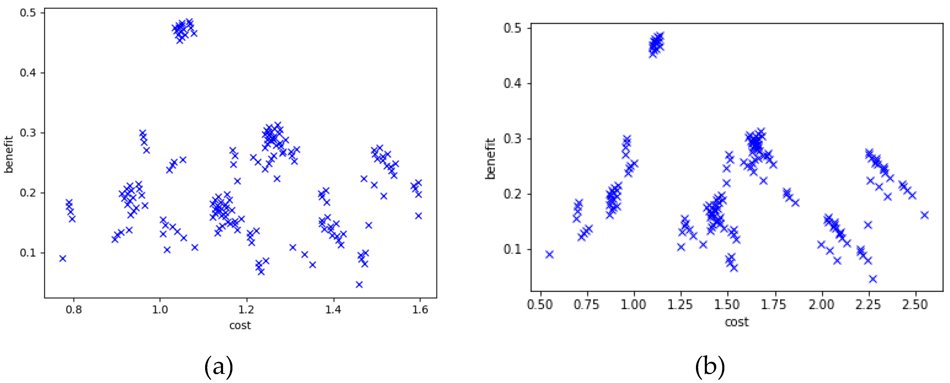
The cost and benefit results of the abovementioned scenarios according to the pre-defined schemes have been analysed by firstly looking at the graphs formed by the scenarios. They have been compared among similar pre-defined schemes. In this paper the analysis performed on three pairs of pre-defined schemes plus scheme 6A are displayed to observe the different point distribution that can exist and the effect that the weighting schemes have on the results. The scenarios presented below correspond to scenarios 1 and 1A, 2 and 2A, 3 and 3A, and 6A. The following Figure 4 shows scenarios 1 and 1A.
When comparing the graphs obtained with pre-defined scheme 1 and with pre-defined scheme 1A, it can be observed that there is a set of scenarios that presents much higher benefit values than the rest in both cases, which corresponds with the scenarios where all measures are applied at the same time, which leads to the achievement of the highest benefits. The majority if scenarios presented have lower benefit values than 0.3, where the highest benefit values are obtained by those where a renewable measure is applied. Additionally, in this group the highest costs are obtained with scenarios where passive external façades, passive roofs and renewables are applied together.
The sets of scenarios can be easily identified, especially in the second case (1A). The reason for this may lay in the higher weight assigned to economic DPIs, which makes cost and benefit results more dependent on them and thus more dependent on the cost of each measure.
Regarding the distribution of the scenarios, in the two schemes it is very similar, but in the case of the scheme 1A the scenarios are more spread in the x-axis (cost) due to the fact that this scheme puts more emphasis in the economic cost.
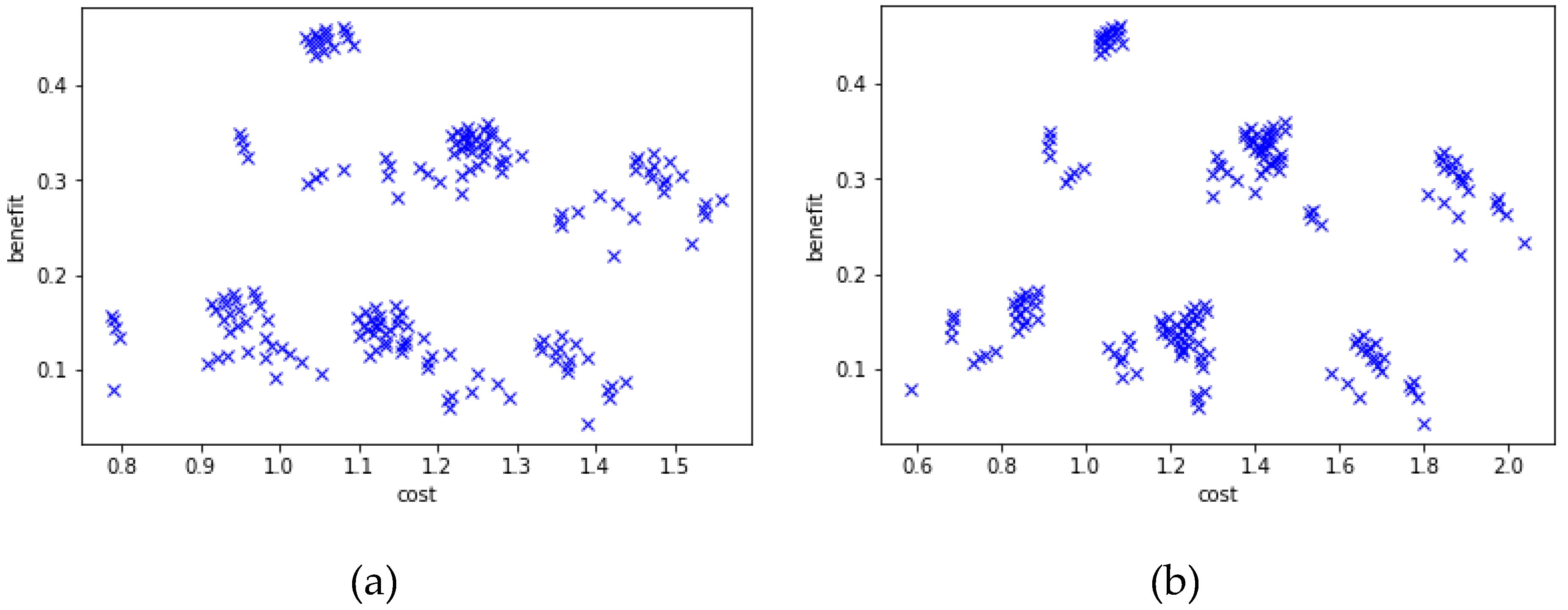
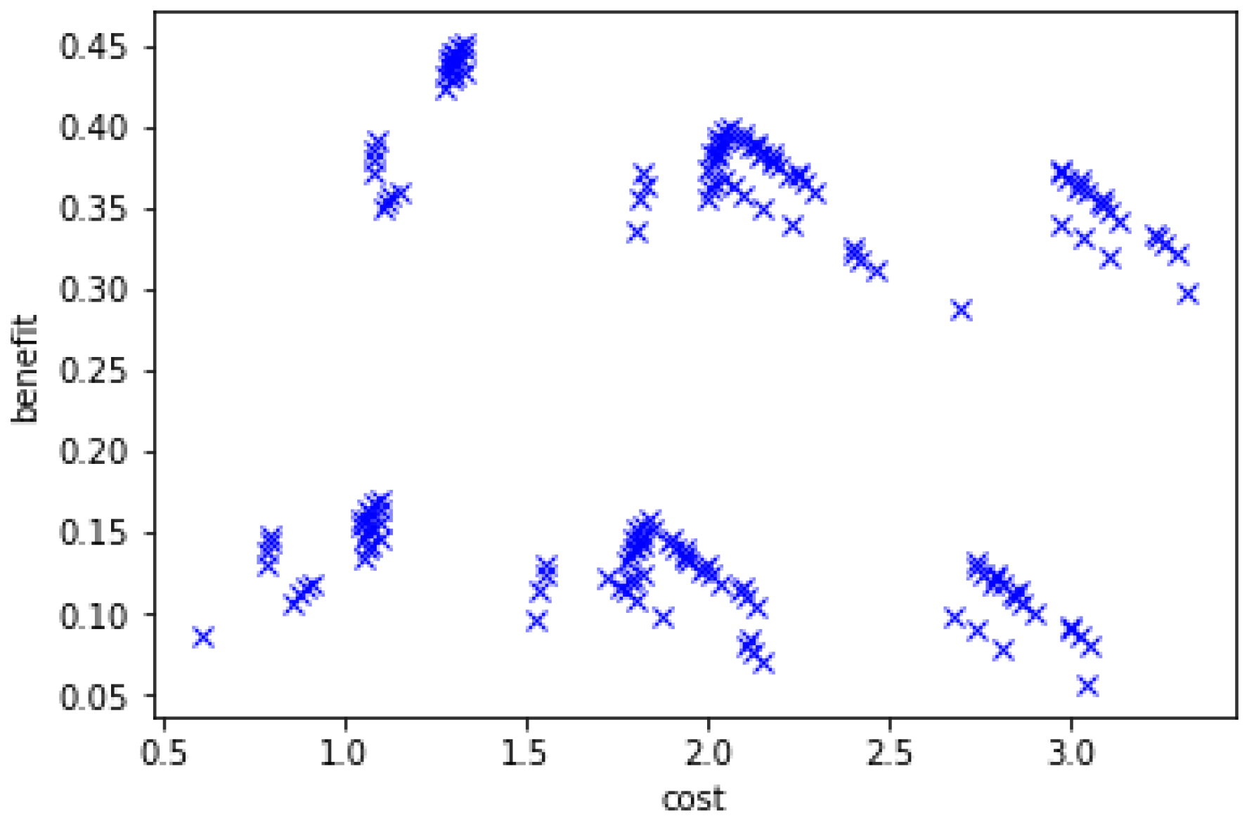
The second pair of scenarios (2 and 2A) corresponds to a priority scheme to achieve a carbon neutral district. The distribution of scenarios is shown in the following Figure 5. As it can be observed within the graphs, there is a set of scenarios that present much higher benefit values than the rest in both cases. These correspond to those that have included passive internal, roof, active and renewable measures applied in an integrated manner. There is one scenario which becomes invariable, with the lowest cost and benefit values, which corresponds to the application of only one active measure.
Also, it can be observed that the benefit values cover a wider range than in the first case, but three main rows appear: the upper row corresponds with the scenarios where all ECMs are applied together; the middle row where a renewable measure is applied in combination with others (P+R, P+A+R, (P ext) + (P roof) + R, (P ext) + (P roof) + A + R, or (P int) + (P roof) + R); whereas in the lower row the rest of the scenarios can be found (passive separately, P+A, Pext +Proof, (P ext) + (P roof) + A, (P int) + (P roof), (P int) + (P roof) + A).
When comparing these two scenarios with the previous (1 and 1A), it can be observed that the point distribution varies, where the cost and benefit values corresponding to the scenarios where passive external and passive roof in combination with active and renewable measures shift to the top, obtaining higher benefit values. This shift can stem from the higher weight given in this pair of prioritisation schemes to the net fossil energy consumed (ENE06) and the energy demand covered by renewable sources (ENE09), which makes scenarios where renewable measures are applied more favourable and, therefore, increasing their benefits.
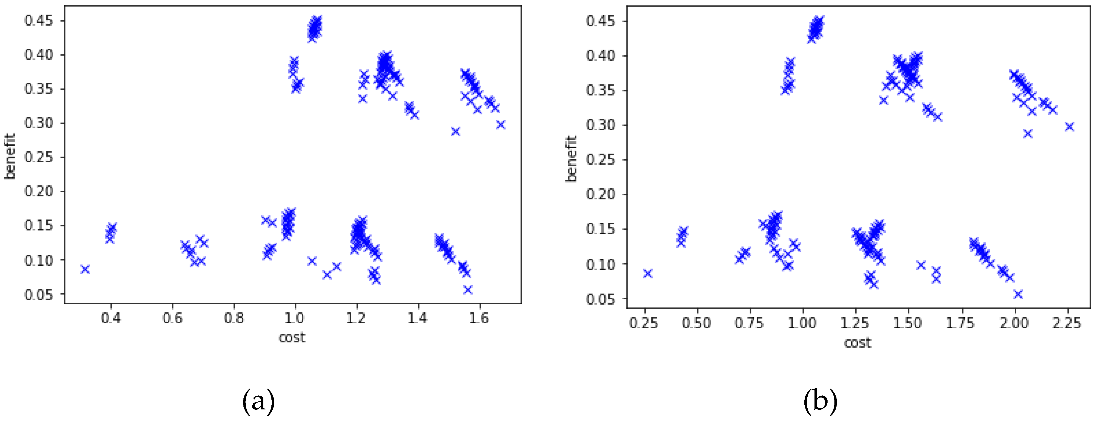
The third pair of scenarios compared corresponds to 3 and 3A, for which the results obtained with the application of their corresponding pre-defined weighting schemes are presented in the following Figure 6:
Comparing pre-defined schemes 3 and 3A it can be concluded that one scenario’s results become invariable, with the lowest cost and benefit values, which corresponds to the application of the active measure separately.
The set of points are divided into two main groups (with the highest or lowest benefit costs): in this set of graphs corresponding to the pre-defined schemes 3 and 3A, the shift towards the top of the scenarios corresponding to passive external and passive roof in combination with active and renewable measures becomes more visible and the difference between cost and benefit values of the scenarios less apparent. The reason for this may lie in the configuration of the prioritisation schemes: in both cases higher weights have been applied to a reduced number of DPIs (in particular ENV06 – energy payback time in the cost’s side and ENE06 (net fossil energy consumed) and ENE09 (energy demand covered by renewable sources), the latter being related to each other.
The sets of scenarios are easily identifiable in both cases. In addition, the sets of scenarios are more clearly identifiable as in the previous cases, having more similar cost and benefit values among each other. Additionally, the cost values are very similar for each set of scenarios where similar ECMs have been applied.
Comparing these two scenarios with the previous it can be shown that the sets of scenarios are more clearly identifiable than in the previous sets of graphs: this implies that small differences in the types of ECMs cannot be fully appreciated, especially in terms of the cost. Shift to the top: higher benefit values are obtained in this scheme for the scenarios where renewables have been applied, which seems logical due to the definition of the scheme: priority to energy generation through renewables.
Finally, the results obtained through applying the pre-defined weighting scheme 6A are shown in Figure 7, where it can be observed that: there are two main groups of scenarios: as in previous cases, there is a great difference among the scenarios where the implementation of renewables is considered (top benefit values) and where they have not (lower values).
For this scheme, groups of scenarios are easily identifiable: as it happened previously, the different sets of scenarios can be easily appreciated. It is to be remarked that especially those with a cost value lower than 1.5 remain quite constant on the cost values, forming vertical lines.
These scenarios correspond to scenarios where the following combinations have been applied: A, P+A, P+A+R, P int + P roof + A and P int + P roof + A +R.

5.2. Pareto Front Observation

Even though some conclusions can be extracted from the visual analysis of these graphs, a closer look at the scenarios that belong to the Pareto front has been performed, in order to check the ones that are displayed to the user at the end of the process.
The first analysis of the graphs enabled the identification of the scenarios belonging to the Pareto front. An analysis of the Pareto fronts obtained was performed based on numerical values where each pair of schemes was compared among each other to detect the major differences.
To serve as a summary of the results obtained through the analysis performed [39] the following table is presented. The different schemes considered are shown, as well as the number of scenarios in their respective Pareto fronts, the targets and boundaries they have reached, together with their maximum and minimum cost and benefit values.
From the table below (Table 10) it can be deduced that the pairs of prioritisation weighting schemes 1 and its complementary economic one (1A) experience an expected variation in the cost values, which sometimes can be highly influential in the cost values obtained and in the number of scenarios in the Pareto front. To this latter aspect, it is also noticeable that a higher number of scenarios appear in the Pareto front for the more economically driven prioritisation schemes (1A, 2A, 3A and 4A).
When comparing the minimum benefit values among each other and the maximum benefit values it can be observed that the deviation among these is not great. However, when doing the same exercise with minimum cost values and maximum cost values, it can be seen that there are major differences.
These can stem from the DPIs considered in each cost and benefit group: whereas in the cost list (ENV01, ENV04, ECO02.2, ECO03 and ECO05) the DPIs are highly different from each other, in the benefits (ENE01, ENE02, ENE06, ENE09, ENE13 and COM01) DPIs evolve in the same direction.
This implies that greater changes will be experienced in the costs whenever a parameter changes in the definition of the scenarios or in the DPI results, whereas in the benefits side, it will remain quite invariable.

6. Conclusions

The platform introduced in this paper offers a tool to stakeholders in order to support them during the decision-making to design energy efficient retrofitting projects at district scale. It provides a comprehensive method in order to make more informed decisions through assessing the performance of the baseline and the candidate retrofitting scenarios against a set of criteria in relevant fields as energy, comfort or economic aspects. This tool automates the generation of these scenarios through combining energy conservation measures, which are selected based on the barriers and priorities established by the user.
A core element of this platform is the evaluation methodology and evaluation tool that has been developed and validated as presented within this paper. This methodology integrates multi-criteria decision analysis methods in order to support building a comprehensive judgement of the district performance under different retrofitting alternatives.
One of the main challenges is the integration of the subjective information coming from stakeholders regarding their priorities and transforming it into quantifiable information that can support the deployment of the appropriate evaluation.
This paper presents an approach to solve this issue through integrating a pairwise comparison method in order to generate the weights that allow building the cost and benefit functions to evaluate and optimise the candidate retrofitting scenarios. This method has led to deploying a set of pre-defined weighting schemes that capture several approaches for energy efficient retrofitting for districts, as prioritising the integration of renewables or the environmental aspects. The method to build the pre-defined weighting schemes has followed the same principles as those that will follow the stakeholders when setting their own priorities to ensure that the evaluation is in line with their expectations.

6.1. Validation of the Evaluation Method

The validations performed have demonstrated the validity of the evaluation method with the results of a series of indicators in scenarios where a determined set of ECMs have been applied.
As input for the evaluation methodology, the prioritisation criteria are needed and the pre-defined weighting schemes developed for the evaluation methodology have been tested. As a conclusion of this analysis the following has been extracted:
  • The cost and benefit functions obtained after evaluating the candidate scenarios with the pre-defined weighting schemes are reasonable.
  • While some pre-defined schemes presented graphs where the point distribution was more spread it is to be highlighted that in schemes such as 3 or 3A (those schemes related to energy generation through renewables) points corresponding to sets of scenarios where the same type of ECM was implemented were more concentrated, indicating that these schemes left little space to appreciate the differences among the same type of ECM.
  • Also noticeable was the great difference between the schemes where renewables were favoured (as schemes 3 or 3A) and the rest. In these first schemes it can be observed that the scenarios where renewables have been applied have greater benefits. This was the main intention of the configuration of the scheme. However, it might be advisable to make the user aware of these facts when applying the pre-defined schemes.
  • For the economically driven prioritisation schemes (1A, or 3A) a higher number of scenarios appear in the Pareto front. It can be deducted that the use of these schemes makes possible to better discriminate scenarios with similar measures by intensifying their main differences.
The analysis of the numerical values of the Pareto front did not provide highly relevant insights to the analysis, since the point distributions and related observations had already been carried out. However, it is to be highlighted that regardless of the scheme, the extreme benefit values do not vary significantly, whereas major differences can be seen in the cost values.
These validations have served for the tool to address more complex cases, evaluating and optimising districts with several buildings covering the complete assessment of the effects among buildings and how the optimisation at district scale can derive into wider benefits than when tackling buildings individually. Under these cases the scale of the optimisation problem rises dramatically and requires enough power in order to compute the simulation models in a reasonable time. This is addressed through techniques as parallel computing in order to cope with the number of models required.

6.2. Limitations and Considerations

As it can be shown within the description of the methodology and its validation, the implementation of this approach is highly dependent on the quality of the input information provided in order to perform both the validation and evaluation of the candidate retrofitting scenarios to effectively support decision making. The quality of the input data is validated through a set of processes that ensure completeness and minimum quality requirements to allow generating the simulation models to launch the tools that integrate the simulation toolbox. However, there is a need for an intensive validation of the accuracy of these data by the user before being inserted into the tool to ensure the district to be evaluated is appropriately represented within the models that capture the situation before implementing the retrofitting project.
Apart from the accuracy of the data, as it can be concluded from the implementation of the various prioritisation schemes, the way in which the candidate scenarios are formulated and ranked depend on an appropriate selection of the priorities to achieve when describing the problem to be addressed by the platform. The tool enables the users selecting from a range of prioritisation weighting schemes or the definition of an own scheme through implementing a pairwise comparison method over the indicators selected for the evaluation. The selection of the importance given to each indicator over the others, which aims at transforming subjective information into an objective mathematical problem to allow identifying the optimal retrofitting scenarios, is therefore a key element to ensure that the best scenarios are those which respond to the boundary conditions that the stakeholders of the retrofitting process have set.

6.3. Future Research Work

Future work could consider the integration of more domains within the evaluation method in order to cover other relevant fields apart from the evaluation of energy efficiency measures. The evaluation method and tool proposed have demonstrated to be flexible and expandable enough in order to ensure an appropriate integration of new developments.
Conclusively, this evaluation method and its integration within the comprehensive platform to deliver services for energy efficient projects design can provide important benefits to the stakeholders, such as enabling more informed and comprehensive decision making, consideration of their priorities in a quantifiable manner, and automation of the evaluation process that reduces time and uncertainties and better integration of stakeholders.

Author Contributions

The contents of this paper have been collaboratively created by the authors, with the following contributions: conceptualisation, methodology, validation, formal analysis, investigation, writing-original draft preparation, writing-review and editing, visualisation, supervision, project administration, and funding acquisition, M.Á.G.-F.; software, validation, formal analysis, data curation, and funding acquisition, V.S.; validation, formal analysis, investigation, and data curation, G.H.; writing-review and editing, and supervision, A.M.

Funding

This research work has been partially funded by the European Commission through the European Union’s Horizon 2020 Research and Innovation Programme under the research project Optimised Design Platform for Refurbishment at District Level (OptEEmAL) with grant agreement No. 680676.

Acknowledgments

The authors would like to thank the rest of the partners for their support. All related information to the project is available at www.opteemal-project.eu.

Conflicts of Interest

The authors declare no conflicts of interest.

Nomenclature

BIMBuilding Information ModellingMCDAMulti-criteria Decision Analysis
IPDIntegrated Project DeliveryAHPAnalytic Hierarchy Process
ECMEnergy Conservation MeasureENEEnergy indicators
DPIDistrict Performance IndicatorCOMComfort indicators
IFCIndustry Foundation ClassesECOEconomic indicators
GUIGraphical User InterfaceENVEnvironmental indicators

References

  1. Directive on the Energy Performance of Buildings (EPBD). Directive 2002/91/EC of the European Parliament and Council on Energy Efficiency of Buildings. Off. J. Eur. Communities 2002, 1, 65–71. [Google Scholar]
  2. Europe’s Buildings under the Microscope; Buildings Performance Institute Europe (BPIE): Bruxelles, Belgium, 2011; ISBN 9789491143014.
  3. Laponche, B.; López, J.; Raoust, M.; Novel, A.; Devernois, N. Energy Efficiency Retrofitting of Buildings: Challenges and Methods; Agence Française de Développement: Paris, France, 2012. [Google Scholar]
  4. Lilis, G.N.; Giannakis KKatsigarakis, K.; Rovas, D.; Costa, G.; Sicilia, A.; García-Fuentes, M. Simulation model generation combining IFC and CityGML data. In Proceedings of the ECCPPM 2016 11th European Conference on Product and Process Modelling, Limassol, Cyprus, 7–9 September 2016. [Google Scholar]
  5. García-Fuentes, M.A.; Pujols, C.; García-Pajares, R.; Vasallo, A.; Martín, A. Metodología de Rehabilitación Energética hacia Distritos Residenciales de Energía Casi Nula. Aplicación al barrio del Cuatro de Marzo (Valladolid). In Proceedings of the II Congreso EECN, Madrid, Spain, 6–7 May 2014. [Google Scholar]
  6. Bryde, D.; Broquetas, M.; Volm, J.M. The project benefits of Building Information Modelling (BIM). Int. J. Proj. Manag. 2013, 31, 971–980. [Google Scholar] [CrossRef]
  7. The American Institute of Architects (AIA) National. Integrated Project Delivery: A Guide; Report; American Institute of Architects, AIA California Council: Sacramento, CA, USA, 2014. [Google Scholar]
  8. OptEEmAL. Available online: www.opteemal-project.eu (accessed on 13 June 2019).
  9. Lilis, G.N.; Giannakis, G.; Rovas, D.V. Inter-building shading calculations based on CityGML geometric data. In Proceedings of the 15th IBPSA Conference, San Francisco, CA, USA, 7–9 August 2017; pp. 370–379. [Google Scholar]
  10. OptEEmAL Partners. D3.1: Requirements and Specification of the ECMs Catalogue. 2016. Available online: https://www.opteemal-project.eu/files/opteemal_d3.1_requirementsspecificationecmscatalogue.pdf (accessed on 9 May 2019).
  11. Industry Foundation Classes (IFC) for Data Sharing in the Construction and Facility Management Industries; ISO 16739; International Organization for Standardization: Geneva, Switzerland, 2013.
  12. Kolbe, T.H.; Gröger, G.; Plümer, L. CityGML: Interoperable Access to 3D City Models. In Geo-Information for Disaster Management; Springer: Berlin/Heiidelberg, Germany, 2005; pp. 883–899. [Google Scholar]
  13. Lilis, G.N.; Giannalis, G.; Rovas, D. District-aware Building Energy Performance simulation model generation from GIS and BIM data. In Proceedings of the BSO 2018 4th Building Simulation and Optimisation Conference, Cambridge, UK, 11–12 September 2018. [Google Scholar]
  14. Bazjanac, V. Space boundary requirements for modeling of building geometry for energy and other performance simulation. In Proceedings of the CIB W78, Cairo, Egypt, 16–19 November 2010. [Google Scholar]
  15. Giannakis, G.; Lilis, G.N.; Garcia-Fuentes, M.A.; Kontes, G.; Valmaseda, C.; Rovas, D. A methodology to automatically generate geometry inputs for energy performance simulation from IFC BIM models. In Proceedings of the Building Simulation IBPSA Conference, Hyderabad, India, 7–9 December 2015; pp. 504–511. [Google Scholar]
  16. Hernández, G.; Serna, V.; García-Fuentes, M.Á. Design of energy efficiency retrofitting projects for districts based on performance optimization of District Performance Indicators calculated through simulation models. Energy Procedia 2017, 122, 721–726. [Google Scholar] [CrossRef]
  17. García-Fuentes, M.Á.; García-Pajares, R.; Sanz, C.; Meiss, A. Novel Design Support Methodology Based on a Multi-Criteria Decision Analysis Approach for Energy Efficient District Retrofitting Projects. Energies 2018, 11, 2368. [Google Scholar] [CrossRef]
  18. Crawley, D.; Lawrie, L.; Pedersen, C.; Winkelmann, F. EnergyPlus: Energy Simulation Program. ASHRAE J. 2000, 42, 49–56. [Google Scholar]
  19. De Tommasi, L.; Ridouane, H.; Giannakis, G.; Katsigarakis, K.; Lilis, G.N.; Rovas, D.; Tommasi, L. Model-Based Comparative Evaluation of Building and District Control-Oriented Energy Retrofit Scenarios. Buildings 2018, 8, 91. [Google Scholar] [CrossRef]
  20. Peyser, A.; Sinha, A.; Vennemo, S.B.; Ippen, T.; Jordan, J.; Graber, S.; Morrison, A.; Trensch, G.; Fardet, T.; Mørk, H.; et al. NEST 2.14.0. Zenodo 2017. [Google Scholar] [CrossRef]
  21. Valderrama-Ulloa, C.; Puiggali, J.R. User requirements in building translated in a methodology of decision support. Inf. Constr. 2014, 66, e022. [Google Scholar] [CrossRef]
  22. Dodgson, J.; Spackman, M.; Pearman, A.; Phillips, L. Multi-Criteria Analysis: A Manual; Communities and Local Government Publications: Wetherby, UK, 2009.
  23. Environmental Management—Lifecycle Assessment: Principles and Framework; ISO14040; International Organization for Standardization: Geneva, Switzerland, 2006.
  24. Pohekar, S.D.; Ramachandran, M. Application of multi-criteria decision making to sustainable energy planning—A review. Renew. Sustain. Energy Rev. 2004, 8, 365–381. [Google Scholar] [CrossRef]
  25. Manjarres, D.; Mabe, L.; Oregi, X.; Landa-Torres, I.; Arrizabalaga, E. A Multi-objective Harmony Search Algorithm for Optimal Energy and Environmental Refurbishment at District Level Scale. In Proceedings of the 3rd International Conference on Harmony Search Algorithm (ICHSA 2017), Bilbao, Spain, 22–24 February 2017; Springer: Berlin/Heidelberg, Germany, 2017. [Google Scholar]
  26. Nemhauser, G.; Rinnooy, A.; Todd, M. (Eds.) Optimization. Handbooks in Operations Research and Management Science; Elsevier: Amsterdam, The Netherlands, 1989; Volume 1. [Google Scholar]
  27. Rowley, H.V.; Peters, G.M.; Lundie, S.; Moore, S.J. Aggregating sustainability indicators: Beyond the weighted sum. J. Environ. Manag. 2012, 111, 24–33. [Google Scholar] [CrossRef] [PubMed]
  28. Coello, C. A Short Tutorial on Evolutionary Multiobjective Optimization; Lecture Notes in Computer Science book series; Springer Nature: Basel, Switzerland, 1993; Volume 1993. [Google Scholar]
  29. Engel, A. Verification, Validation and Testing of Engineered Systems; Wiley Series in Systems Engineering and Management; Wiley: Hoboken, NJ, USA, 2010. [Google Scholar]
  30. Ebert, U.; Welsch, H. Meaningful environmental indices: A social choice approach. J. Environ. Econ. Manag. 2004, 47, 270–283. [Google Scholar] [CrossRef]
  31. Barba-Romero, S.; Pomerol, J.C. Decisiones Multicriterio: Fundamentos Teóricos y Utilización Práctica; Universidad de Alcalà: Madrid, Spain, 1995. [Google Scholar]
  32. Kima, D.O.; Ramina, M.; Chenga, V.; Javeda, A.; Kaluskara, S.; Kellya, N.; Kobilirisa, D.; Neumanna, A.; Nia, F.; Pellera, T.; et al. An integrative methodological framework for setting environmental criteria: Evaluation of stakeholder perceptions. Ecol. Inform. 2018. [Google Scholar] [CrossRef]
  33. Boyssou, D.; Marchant, T.; Pirlot, M.; Tsoukiàs, A.; Vincke, P. Evaluation and Decision Models with Multiple Criteria: Stepping Stones for the Analyst; Springer: New York, NY, USA, 2006. [Google Scholar]
  34. Song, B.; Kang, S. A Method of Assigning Weights Using a Ranking and Nonhierarchy Comparison. Adv. Decis. Sci. 2016, 2016, 1–9. [Google Scholar] [CrossRef] [Green Version]
  35. Saaty, T.L. Decision making with the analytic hierarchy process. Int. J. Serv. Sci. 2008, 1, 83. [Google Scholar] [CrossRef] [Green Version]
  36. Klutho, S. Mathematical Decision Making: An Overview of the Analytic Hierarchy Process. 2013. Available online: https://www.whitman.edu/Documents/Academics/Mathematics/Klutho.pdf (accessed on 13 June 2019).
  37. OptEEmAL Partners. D4.4: Requirements and Design of the Simulation Model Input Generator, 2016.
  38. García-Fuentes, M.; Serna, V.; Hernández, G. Evaluation and optimisation of energy efficient retrofitting scenarios for districts based on district performance indicators and stakeholders’ priorities. In Proceedings of the Building Simulation and Optimisation 2018, Cambridge, UK, 11–12 September 2018. [Google Scholar]
  39. OptEEmAL Partners. D4.3: Validation of the Optimisation Module, 2017.
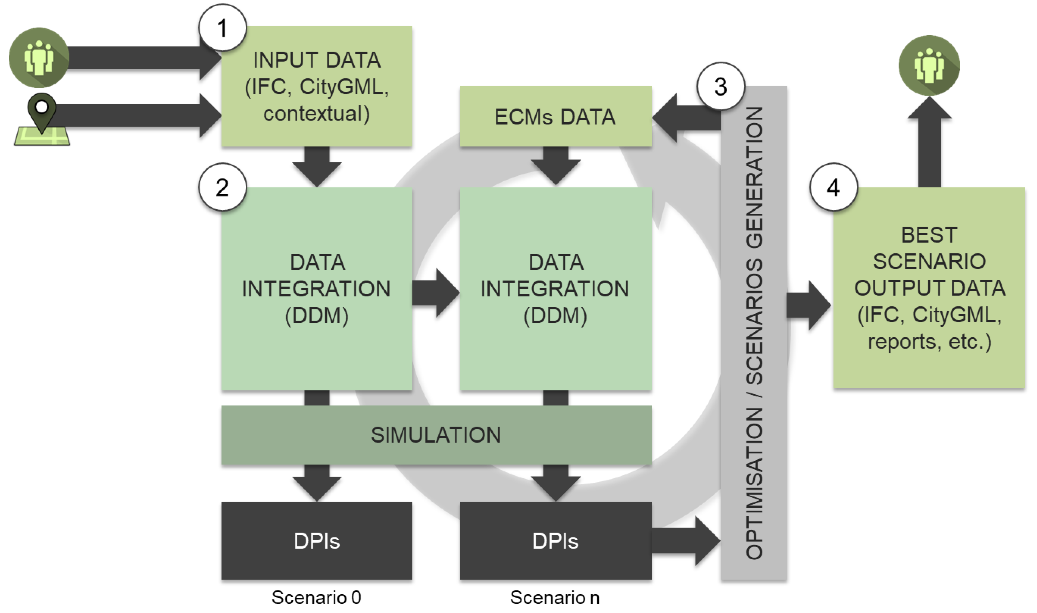
Figure 1. Platform process. Adapted from [16].
Applsci 09 02448 g001
Figure 2. Scheme of the evaluation process.
Applsci 09 02448 g002
Figure 3. Hierarchy for the decision-making process.
Applsci 09 02448 g003
Figure 4. Pre-defined scheme 1 (achieve a nearly zero energy district) (a) and pre-defined scheme 1A (achieve a nearly zero energy district + economic aspects) (b).
Applsci 09 02448 g004
Figure 5. Pre-defined scheme 2 (achieve a carbon neutral district) (a) and pre-defined scheme 2A (achieve a carbon neutral district + economic aspects) (b).
Applsci 09 02448 g005
Figure 6. Pre-defined scheme 3 (energy generation through renewables) (a) and pre-defined scheme 3A (energy generation through renewables + economic aspects) (b).
Applsci 09 02448 g006
Figure 7. 6A (environmental issues + economic aspects).
Applsci 09 02448 g007
Table 1. List of District Performance Indicators (DPIs) per evaluation group.
Group 1—CostGroup 2—Benefit 1Group 3—Benefit 2
ENV01.Global Warming Potential - GWP (kg CO2) ENE 01.Energy demandENE 14.Energy use from Biomass
ENV04.Primary energy consumptionENE02.Final energy consumptionENE 15.Energy use from PV
ENV06.Energy payback timeENE 06.Net fossil energy consumed ENE 16.Energy use from Solar Thermal
ECO02.2 Investments (in €)ENE 09.Energy demand covered by renewable sourcesENE 17.Energy use from Hydraulic
ECO03.Life cycle costENE 13.Energy use from District HeatingENE 18.Energy use from Mini-Eolic
ECO05.Payback PeriodCOM01.Local thermal comfortENE 19.Energy use from Geothermal
Table 2. The fundamental scale of absolute numbers. Adapted from [35].
Intensity of ImportanceDefinitionExplanation
1Equal importanceThe two criteria present the same importance for the participants
3Moderate importanceThe criteria is slightly more important than the one against it is compared
5Strong importanceThe criteria is strongly more important than the one against it is compared
7Very strong importanceThe criteria is very strongly more important than the one against it is compared
9Extreme importanceThe criteria reaches the highest importance, leaving the one against it is compared with negligible importance
Reciprocals of aboveWhen comparing one criteria with a second, the importance of the second over the first is the reciprocal value of the first over the second
Table 3. Pairwise comparison matrices for Matrix 1 (cost).
MATRIX 1: COSTENV03ENV04ENV06ECO02ECO03ECO05
ENV031ENV03/ENV04ENV03/ENV06ENV03/ECO02ENV03/ECO03ENV03/ECO05
ENV04ENV04/ENV031ENV04/ENV06ENV04/ECO02ENV04/ECO03ENV04/ECO05
ENV06ENV06/ENV03ENV06/ENV041ENV06/ECO02ENV06/ECO03ENV06/ECO05
ECO02ECO02/ENV03ECO02/ENV04ECO02/ENV061ECO02/ECO03ECO02/ECO05
ECO03ECO03/ENV03ECO03/ENV04ECO03/ENV06ECO03/ECO021ECO03/ECO05
ECO05ECO05/ENV03ECO05/ENV04ECO05/ENV06ECO05/ECO02ECO05/ECO031
Table 4. Pairwise comparison matrices for Matrix 2 (Benefits Level 1).
MATRIX 2: BENEFITS 1ENE01ENE02ENE06ENE09ENE13COM01
ENE011ENE01/ENE02ENE01/ENE06ENE01/ENE09ENE01/ENE13ENE01/COM01
ENE02ENE02/ENE011ENE02/ENE06ENE02/ENE09ENE02/ENE13ENE02/COM01
ENE06ENE06/ENE01ENE06/ENE021ENE06/ENE09ENE06/ENE13ENE06/COM01
ENE09ENE09/ENE01ENE09/ENE02ENE09/ENE061ENE09/ENE13ENE09/COM01
ENE13ENE13/ENE01ENE13/ENE02ENE13/ENE06ENE13/ENE091ENE13/COM01
COM01COM01/ENE01COM01/ENE02COM01/ENE06COM01/ENE09COM01/ENE131
Table 5. Pairwise comparison matrices for Matrix 3 (Benefits Level 2).
MATRIX 3: BENEFITS 2ENE14ENE15ENE16ENE17ENE18ENE19
ENE141ENE14/ENE15ENE14/ENE16ENE14/ENE17ENE14/ENE18ENE14/ENE19
ENE15ENE15/ENE141ENE15/ENE16ENE15/ENE17ENE15/ENE18ENE15/ENE19
ENE16ENE16/ENE14ENE16/ENE151ENE16/ENE17ENE16/ENE18ENE16/ENE19
ENE17ENE17/ENE14ENE17/ENE15ENE17/ENE161ENE17/ENE18ENE17/ENE19
ENE18ENE18/ENE14ENE18/ENE15ENE18/ENE16ENE18/ENE171ENE18/ENE19
ENE19ENE19/ENE14ENE19/ENE15ENE19/ENE16ENE19/ENE17ENE19/ENE181
Table 6. Weighting of indicators to build the cost–benefit functions.
DPI CodeWeight (wi)RangeObjectiveDPI for Scenario x fi(x)Normalised DPI for Scenario x Ii(x)Weighted and Normalised DPI
min (fi_min)max (fi_max)
ENEi w E N E i 0 1001 f E N E i ( x ) I E N E i ( x ) = f E N E i ( x ) 100 w E N E i · I E N E i ( x )
COMi w C O M i 0 1001 f C O M i ( x ) I C O M i ( x ) = f C O M i ( x ) 100 w C O M i · I C O M i ( x )
ECOi w E C O i 0 f E C O i _ m a x 0 f E C O i ( x ) I E C O i ( x ) = 1 f E C O i ( x ) 100 w E C O i · I E C O i ( x )
ENVi w E N V i 01001 f E N V i ( x ) I E N V i ( x ) = f E N V i ( x ) 100 w E N V i · I E N V i ( x )
Table 7. Description of the case study.
PropertyValuePicture
SurfaceWall surface: 75.60 m2 Applsci 09 02448 i001
Roof surface: 48.00 m2
Spaces1
Elements4 walls
1 roof
0 windows
Table 8. List of scenarios generated for the validation.
ScenariosNumberConcept
11REach renewable (R) measure separately
21AEach active (A) measure separately
3–1412PEach passive (P) measure separately
15–2612P + REach passive measure separately + renewable
27–3812P + AEach passive measure separately + active
39–5012P + A + REach passive measure separately + renewable + active
51–6616(P ext) + (P roof)External passive measure (P ext) + roof insulation (P roof)
67–8216(P ext) + (P roof) + RExternal passive measure + roof insulation + renewable
83–9816(P ext) + (P roof) + AExternal passive measure + roof insulation + active
99–11416(P ext) + (P roof) + A + RExternal passive measure + roof insulation + active + renewable
115–13016(P int) + (P roof) Internal passive measure (P int) + roof insulation
131–14616(P int) + (P roof) + RInternal passive measure + roof insulation + renewable
147–16216(P int) + (P roof) + AInternal passive measure + roof insulation + active
163–17816(P int) + (P roof) + A + RInternal passive measure + roof insulation + active + renewable
Table 9. List of tools used to calculate the indicators.
TypeNameTool
CENV01: Global Warming PotentialNEST
CENV04: Primary energy consumption
CENV06: Energy payback time
CECO02.2: InvestmentsAd-hoc developed tool for economic assessment
CECO03: Life cycle cost
CECOO05: Payback period
B (1)ENE01: Energy demandEnergy Plus and Ad-hoc developed tool for HVAC and control simulation
B (1)ENE02.0: Final energy consumption
B (1)ENE06: Net fossil energy consumed
B (1)ENE09: Energy demand covered by renewable sources
B (1)ENE13: Energy use from District Heating
B (1)COM01: Local thermal comfort
B (2)ENE14: Energy use from biomass
B (2)ENE15: Energy use from PV
B (2)ENE16: Energy use from Solar Thermal
B (2)ENE17: Energy use from hydraulic
B (2)ENE18: Energy use from mini-eolic
B (2)ENE19: Energy use from geothermal
Table 10. Summary of Pareto front and cost and benefit value observation.
SchemeNumber of ScenariosMin. Benefit ValueMax. Benefit ValueMin. Cost ValueMax. Cost Value
1110,0470,4860,7741,597
1A200,0470,4860,5492,545
290,0430,4600,7881,558
2A190,0430,4600,5862,035
3200,0570,4510,3141,669
3A240,0570,4510,2652,259
4200,0570,5330,3141,669
4A240,0570,5330,2652,259
6A200,0570,4510,6043,323