Article

The Impacts of Random Distributed Vacancy Defects in Steady-State Thermal Conduction of Graphene

1
Department of Computational Science and Statistics, School of Science, Nantong University, Nantong 226019, China
2
School of Transportation and Civil Engineering, Nantong University, Nantong 226019, China
3
Département Mécanique, Institut national des sciences appliquées de Rouen, 76801 Rouen, France
*
Author to whom correspondence should be addressed.
Appl. Sci. 2019, 9(11), 2363; https://doi.org/10.3390/app9112363
Submission received: 21 April 2019 / Revised: 3 June 2019 / Accepted: 3 June 2019 / Published: 10 June 2019
(This article belongs to the Section Nanotechnology and Applied Nanosciences)

Abstract

:
The unavoidable vacancy defects dispersed throughout the entire pristine graphene tailor to the integrity of the lattice structure and thereby have complicated impacts on the mechanical and thermal properties of graphene. In order to analyze the influence of vacancy defects on the extraordinary thermal conductivity of graphene, three typical kinds of vacancy defects—namely center concentrated, periodic, and random distributed vacancy defects—are compared and discussed. In the steady-state thermal conduction, the finite element method (FEM) is performed to calculate the total thermal energy and temperature field. The equivalent coefficient of thermal conductivity is derived from thermal energy, amount of vacancy defects, and boundary condition. The chirality in graphene is discussed by the location of its heat source. Moreover, the Monte Carlo simulation is applied to propagate the uncertainty of random vacancy defects in the finite element model of pristine graphene. In this paper, we provide the robustness to defend the impacts of vacancy defects on thermal conduction and the fluctuation and divergence caused by a certain number of random vacancy defects.

1. Introduction

The capability of heat conduction in materials is rooted in its atomic structure. Carbon materials form a variety of allotropes. The allotropes of carbon have completely different orders of magnitude in thermal conductivity, from 0.01 W/mK in amorphous carbon to 2000 W/mK in diamond or graphene in room temperature [1,2]. The mechanical exfoliation of graphene [3] and discovery of its extraordinary electrical conduction [4,5,6] provide strong evidence of thermal transportation in two-dimensional (2D) crystals.
Thermal conductivity is one of the essential issues in the exploration and development of optoelectronic and photonic devices. In the integrated circuits and three-dimensional electronics, thermoelectric energy conversion strongly suppressed thermal conductivity [7]. From the measurement of optothermal Raman in suspended graphene from mechanical exfoliation, the value of thermal conductivity is found to exceed 3000 W/mK [8,9,10]. The phonon mean-free path was estimated to be 775 nm near room temperature [11]. For high-quality chemical vapor deposited (CVD) graphene, the thermal conductivity is also beyond 2500 W/mK at 350 K and is as high as 1400 W/mK at 500 K [12]. When the environmental temperature is at 600 K, the thermal conductivity becomes 630 W/mK for suspended graphene [13]. The range in the interval from 1500–5000 W/mK is reported for the thermal conductivity of suspended graphene [14].
In the investigation process, theoretical and analytical methods are available alternatives of experimental measurements. The theoretical results obtained for heat conduction can be tested and compared with the experiments of high-quality suspended graphene with few layers [15,16,17,18]. Previously, graphene’s thermal conductivity was computed using relaxation-time approximation (RTA) [19]. Based on the Klemens theory, thermal conductivity is predicted with divergence in layer, grain size, and substrate [20,21]. In addition, the molecular dynamics (MD) simulation also provided 9000 W/mK for graphene near room temperature [22]. Heat conduction in graphene nanoribbons with uncertain length, existence of edge roughness, and unavoidable defect concentration has Tersoff and Brenner potential, [23,24,25,26,27,28]. The rough edges in graphene contribute to the reduction of thermal conductivity by orders of magnitude [29,30]. Usually, theoretical description of thermal properties of graphene closely corresponds to that of carbon nanotubes [31].
The extraordinary thermal conductivity of graphene is confirmed both in experimental measurements and theoretical analysis results. However, there are still challenging issues. First, whether the contribution and importance of Z axial acoustic phonons in graphene is negligible [32,33] or dominant, it is still not clearly defined. Second, thermal conductivity non-linearly depends on the temperature [34], which is proofed in the experimental [35] and theoretical [36] data. Third, the optical absorption under the conditions of the experiment [37] leads to underestimated thermal conductivity. It is hard to compare directly its accuracy of Raman optothermal technique with that of the thermal-bridge or 3-ω techniques [38,39,40,41]. Lastly, the parameters of geometrical properties are ambiguous and the defects are difficult to precisely define. Based on the inter-atomic potential [42], the graphene thickness equals 0.34 nm, but based on Young’s modulus and tensile strength [43], the thickness ranges from 0.06–0.69 nm. The inevitable vacancy defects dispersed throughout the entire pristine graphene tailor to the integrity of the lattice structure and impact the thermal conductivity of graphene. It is necessary to quantitatively analyze the influence of vacancy defects in graphene’s thermal conduction.
In this paper, three typical kinds of vacancy defects—namely center concentrated, periodic, and random distributed vacancy defects—are introduced in the pristine graphene. The chirality of graphene is considered by using the boundary condition as a location of its heat source. In steady-state thermal conduction, the finite element method (FEM) is performed to calculate the total thermal energy and temperature field in graphene. The equivalent coefficient of thermal conductivity is derived from thermal energy, amount of vacancy defects, and boundary condition. Moreover, the Monte Carlo simulation is applied to propagate the uncertainty of random vacancy defects in the finite element model of pristine graphene. The results are discussed and analyzed comprehensively.

2. Materials and Methods

Heat is transferred through two different modes: elastic crystal lattice vibrations of atoms or molecules and collision between particles caused by free electrons movability. The impurities and defects cause structure heterogeneity, destroy the continuums, and bring about electron scattering. The thermal conductivity sharply declines in the appearance of impurities and defects. For quantitative analysis of the impacts of vacancy defects on graphene, the finite element method is applied in the steady-state thermal conduction.

2.1. Steady-State Thermal Conduction

Consider that the volume of an element is and the quantity of the heat entering in time δ τ is δ Q x . According to Fourier’s heat conduction equation, the temperature T is a function of x, y, z, and time τ . The unidirectional heat flow can be written as:
δ Q x = K x ( δ y δ z ) T x δ τ
where K x is the conductivity constant in the x direction and the lengths of the volume elements in y and z direction are represented as δ y , δ z respectively. The leaving quantity of heat can be expressed by Taylor’s series as:
δ Q x + δ x = δ Q x + x ( δ Q x ) δ x + ε
Excluding the high order terms ε , the net heat inflow in x direction can be approximately computed as:
δ Q x δ Q x + δ x = x [ K x ( δ y δ z ) T x δ τ ] δ x = [ x ( K x T x ) ] δ V δ τ
where δ V = δ x δ y δ z is the volume. According to the heat inflow in x direction, the sum of the net amount of heat stored due to difference in conduction heat flow can be expressed as:
δ Q = [ x ( K x T x ) + z y ( K y T y ) + z ( K z T z ) ] δ V δ τ
K y , K z are the conductivity constants in the y and z direction, respectively. Besides, the heat generation in the element at a rate of per unit volume per unit time is introduced as q g :
x ( K x T x ) + y ( K y T y ) + z ( K z T z ) + q g = ρ c T τ
For homogeneous materials, K x = K y = K z . When there is no heat generation q g = 0 , the above equation is simplified as:
2 T x 2 + 2 T y 2 + 2 T z 2 = 1 α T τ
For the steady-state heat conduction, the derivative of the temperature with time is zero. Then, the heat conduction equation can be written as:
2 T x 2 + 2 T y 2 + 2 T z 2 + q g K = 0

2.2. Thermal Conductivity

The thermal conductivity in matter is one of the natural properties. For graphene, optothermal Raman, and electrical measurements are performed to test the thermal conductivity of suspended graphene layers from exfoliation or chemical vapor deposition (CVD). Besides, MD numerical simulation and analytical methods based on the Boltzmann transport equation in valence force field are explored to determine the precise value of thermal conductivity. In Table 1, the ranges of thermal conductivity for graphene are listed from different experimental tests and simulation methods. Large deviation is demonstrated for thermal conductivity from 600 W/mK to 10000 W/Mk. However, the results of Nika [21,36], Savin [25] and Lindsay [31] are more approximated consistent to the measurements results of Balandin [8], Ghosh [10], Jaugeras [14], and Cai [12] than the result of MD [29], as shown in Figure 1. Therefore, the values of thermal conductivity for graphene are settled in the reported range of Balandin [8] and Nika [21].
The heat in graphene is mostly carried by acoustic phonons rather than by electrons. The heat flux along a graphene flake can be computed as [21]:
W = s , q v ( s , q ) ω s ( q ) N ( q , ω s ( q ) ) = s , q v ( s , q ) ω s ( q ) n ( q , ω s )
The above equation can be used to calculate the thermal conductivity with the actual dependence on the phonon frequency ω s ( q ) , the phonon velocity v ( s , q ) , and the number of the phonon with the certain frequencies n ( q , ω s ) . v ω is the energy carried by one phonon and N ( ω , q ) is the number of phonons in the heat flux. From the macroscopic definition:
W α = κ α β ( T ) β h L x L y
where L x = d is the width of graphene flake, L y is the sample length, and h is supposed to be 0.35 nm as the thickness of graphene. The thermal conductivity tensor κ α β in Equation (9) is expressed as:
κ α β = 1 h L x L y s , q τ t o t ( s , q ) v α ( s , q ) v β ( s , q ) N 0 ( ω s ) T ω s ( q )
where τ t o t is the combined phonon relaxation rate in graphene. Moreover, α , β are the subscripts that represent the elements in the matrix of thermal conductivity tensor. Similarly, the diagonal element of the thermal conductivity tensor is computed as:
κ α α = 1 h L x L y s , q τ t o t ( s , q ) v 2 ( s , q ) cos 2 φ N 0 ( ω s ) T ω s ( q )
Then, the 2D density of phonon states is taken into consideration to obtain the expression for the scalar thermal conductivity:
κ = 1 4 π k T 2 h s = 1 6 0 q max { [ ω s ( q ) v s ( q ) ] 2 τ t o t ( s , q ) E x p ( ω s ( q ) / k T ) ( E x p ( ω s ( q ) / k T ) 1 ) 2 q } d q
Based on Equation (12), the dispersion of phonon and phonon polarization branches are taken into consideration using a valence force field. The room temperature is substituted into the theoretical expression of Equation (12). Then, the value of thermal conductivity in this study is set to be 3000 W/mK for steady-state heat conduction.

2.3. Finite Element Model for Graphene

FEM is applied for spatial discretization. In the weighted residual method, trial functions serve as weighting functions. In the finite element model, the conducting bars in graphene lattice is defined by two nodes, a cross-sectional area, and the material properties, as in Figure 2. Specific heat and density are ignored for steady-state solutions. The thermal conductivity is in the element longitudinal direction.
The conductivity matrix of element can be expressed as:
[ K e ] = A K L [ 1 1 1 1 ]
where A, K, and L is the area, thermal conductivity, and distance between nodes, respectively.
The output is computed as:
q = K ( T i T j ) L
Q = q A
where q , T i , T i , and Q is the thermal flux, temperature at node i and j, and Q is the heat rate.
Energies are available in the solution for each element.
E e p o = { 1 2 i = 1 N { σ } T { ε e i } v o l i + E e p i + E s 1 2 { u e } T ( [ K e ] + [ S e ] ) { u e }
where N is the number of integration points, { σ } is the stress vector, { ε e i } is the elastic strain vector, v o l i of integration point i , E e p i is the plastic strain energy, E s is the stress stiffening energy.
E s = { 1 2 { u e } T [ S e ] { u e } 0
where [ K e ] is the element stiffness or conductivity matrix. [ S e ] is the element stress stiffness matrix. { u e } is element degree of freedom vector.
Figure 3 shows the finite element model based on honeycomb lattice structure of graphene. Its heat source is discussed in armchair and zigzag edges, respectively, as shown in Figure 3a,b. The colorful contour depicts the thermal conduction in the steady-state.
Vacancy defects are an unavoidable existence in graphene. However, the shape, size, and location in the entire graphene are unpredictable and uncertain. In order to discuss the impacts of vacancy defects in the steady-state thermal conduction of graphene, three different vacancy defects are compared and discussed in the following results. As shown in Figure 4, center concentrated vacancy defects, periodic vacancy defects, and random distributed vacancy defects are included as three typical vacancy defects in graphene.

3. Results and Discussion

In the following section, the three kinds of vacancy defects are sequentially presented.

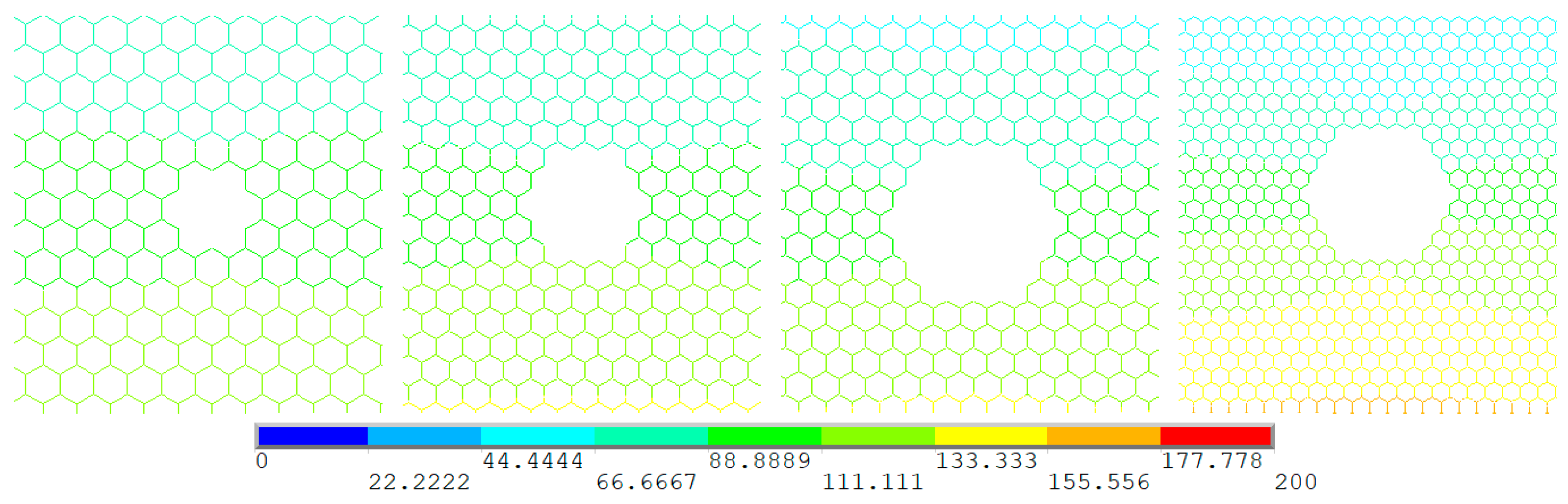
3.1. Center Concentrated Vacancy Defects

The concentrated vacancy defects in the center of graphene are gradually amplified, as shown in Figure 5. According to the size amplification of the center concentrated vacancy defects, the thermal energy of entire graphene gradually decreases in both situations, no matter what its heat source is in the armchair or zigzag edges. The thermal energy of graphene with its heat source in armchair edges is larger than that of graphene with its heat source in zigzag edges, as shown in Figure 6a. The location of its heat source, as one of the boundary conditions, contributes to the difference of thermal energy in the steady-state thermal conduction of graphene. Furthermore, the definition of equivalent coefficient of thermal conductivity for vacancy defected graphene can be expressed as:
C = i = 1 m E i T / m i = 1 n E p i T / n
In addition, the percentage of vacancy defects in the entire graphene can be counted as:
P e r = n m n × 100 %
where n and m are the number of elements in pristine graphene and vacancy defected graphene. The total thermal energy is computed by the sum of the thermal energy of each element and E p i T in pristine graphene and vacancy defected graphene, independently.
Based on Equation (18), the amount of vacancy defects is introduced in an equivalent coefficient of the thermal conduction. In Figure 6b, the reduction of an equivalent coefficient of thermal conductivity becomes sharper with the size amplification of a concentrated center. Under both boundary conditions, the impact of vacancy defects in a steady-state thermal conduction is non-linear. Further, the gradient of curve in the equivalent coefficient is augmented with the enlargement of center concentrated vacancy defects. Moreover, the vacancy defected graphene sheets with its heat source in armchair and zigzag edges have consistent results in the thermal condition’s equivalent coefficient, especially when the size of the center concentrated vacancy defects is not large. With the size enlargement of the center concentrated vacancy defects, the difference between two boundary conditions becomes evident. The graphene with its heat source in armchair edges has higher equivalent coefficient of thermal conductivity than that with its heat source in zigzag edges.
In addition, the contour of temperature in graphene is revealed in Figure 7 and Figure 8. In order to track the exact impacts of center concentrated vacancy defects in the steady-state heat conduction of graphene, the local region around the center concentrated vacancy defects is compared. When the size of the vacancy defects is small, the effects in temperature are not obvious. Along with the size amplification of center concentrated vacancy, the influenced region in graphene become larger and the regularity and band characteristic of temperature results in pristine graphene is destroyed under both boundary conditions. The regions close to the center concentrated vacancy defects tend to have a higher temperature than the pristine graphene. Therefore, the center concentrated vacancy defects in graphene is a crucial factor to change the temperature field in the steady-state thermal conduction. Heat accumulation near the center concentrated vacancy defects in graphene leads to local higher temperature and can cause thermal damages in devices.

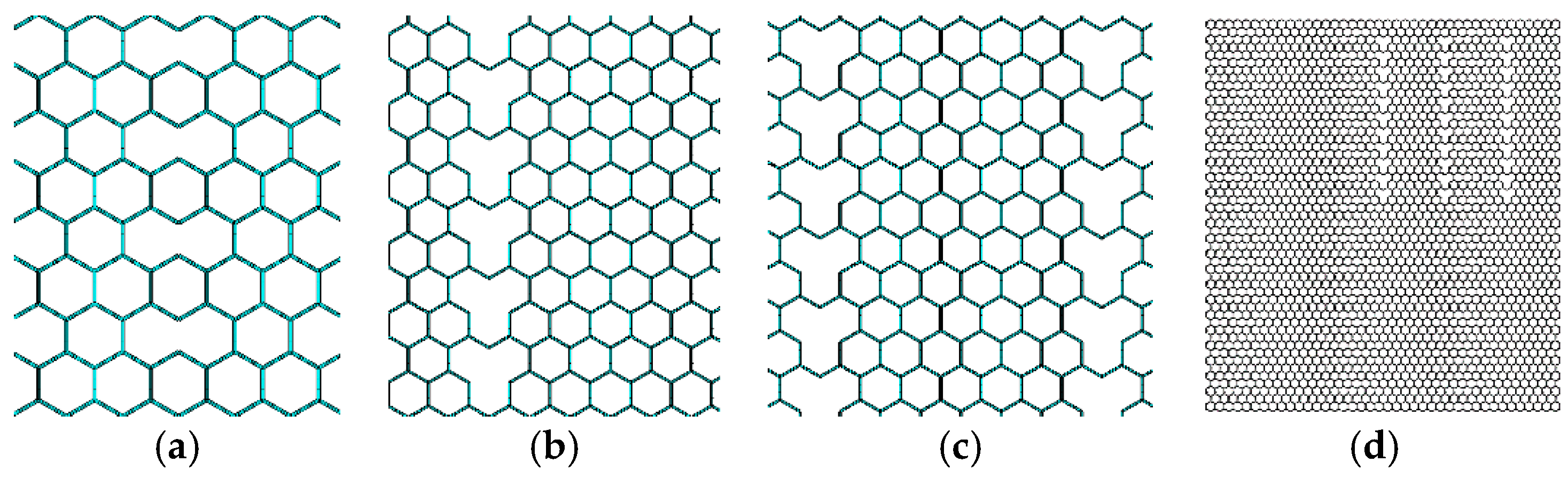
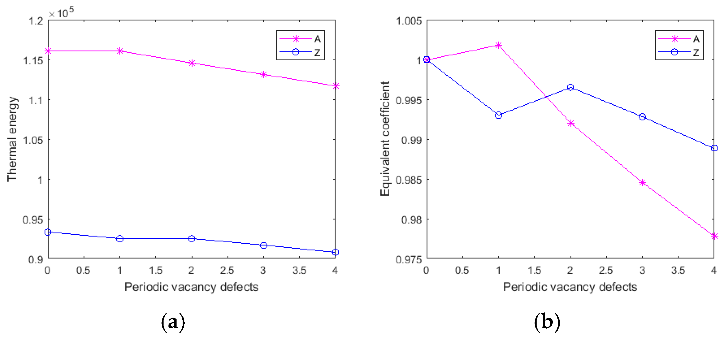
3.2. Periodic Vacancy Defects

Different with the pattern of center concentrated vacancy defects, periodic vacancy defects are gradually dispersed in one quarter of a graphene sheet, as presented in Figure 9. The thermal energy and equivalent coefficient of thermal conductivity are computed by the finite element model in graphene with its heat source in armchair and zigzag edges.
With the increase in the amount of periodic vacancy defects, the thermal energy in graphene with its heat source in the armchair and zigzag edges generally decrease. The thermal energy in the graphene with heat source in the armchair edges are absolutely larger than that in the graphene with its heat source in zigzag edges. However, the results of the equivalent coefficient of thermal conductivity is more complicated than that of the center concentrated vacancy defects, as shown in Figure 10. The equivalent coefficient of the thermal conductivity in graphene with its heat source in armchair edges has a strengthening effect, owing to periodic vacancy defects. Furthermore, the equivalent coefficient of thermal conductivity in graphene with its heat source in zigzag edges does not monotonically decrease with the development of periodic vacancy defects. The fluctuation exists in the second mode of periodic vacancy defects.
Contrary to graphene with its heat source in armchair edges, graphene with its heat source in zigzag edges has an apparent reduced equivalent coefficient of thermal conductivity in the first mode of periodic vacancy defects. Although thermal energy of graphene with its heat source in armchair edges is larger than that of graphene with its heat source in zigzag edges in all modes of periodic vacancy defects, graphene with its heat source in zigzag edges has greater equivalent coefficient of thermal conductivity after the first mode. Thus, graphene with its heat source in armchair edges has a strengthening effect caused by the first mode of periodic vacancy defects. However, it decreases abruptly with the development of periodic vacancy defects, while graphene with its heat source in zigzag edges is more robust and defends against the effects of periodic vacancy defects with fluctuation.
Moreover, the influence of periodic vacancy defects in the temperature field is not as evident as that in the center concentrated vacancy. In Figure 11 and Figure 12, the changes in the temperature field of the local region near the periodic vacancy defects in graphene with its heat source in armchair and zigzag edges are not obvious when compared with the results in the original pristine graphene.

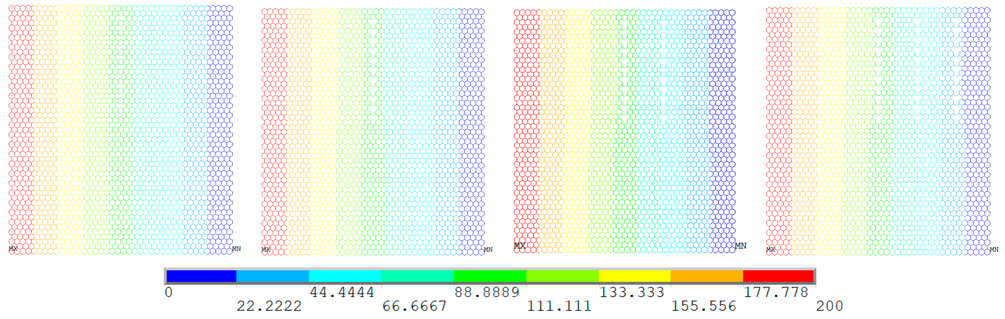
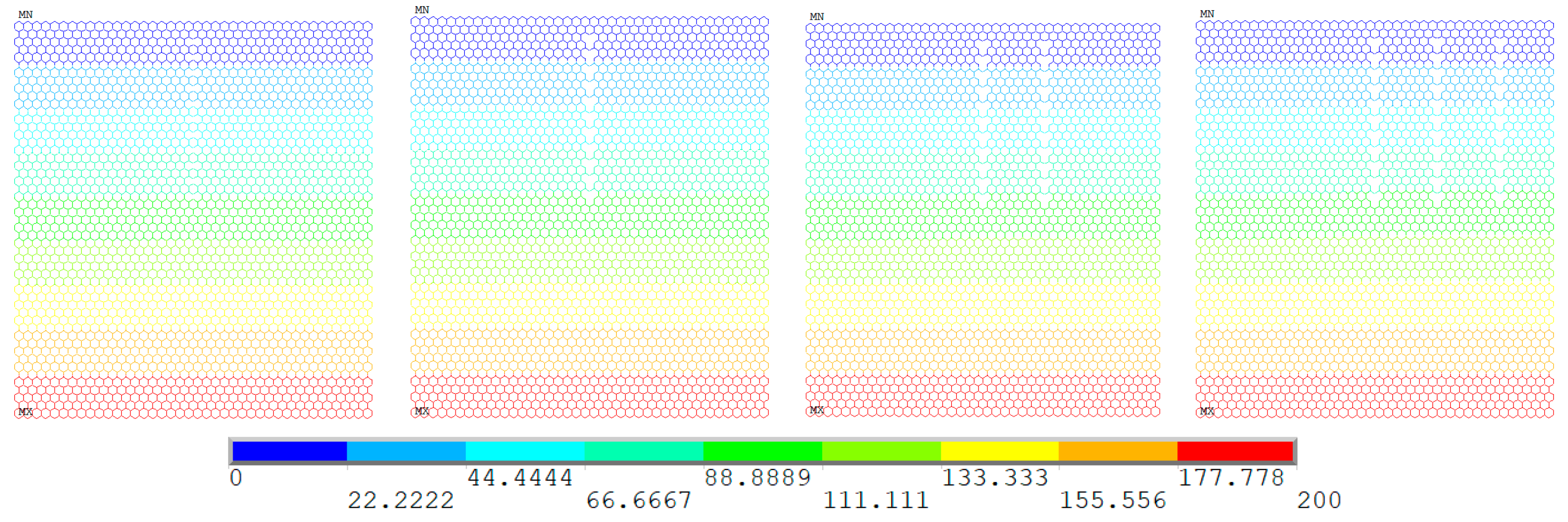
3.3. Random Distributed Vacancy Defects

The center concentrated and periodic vacancy defects are two typical vacancy defects in graphene. Actually, the vacancy defects are stochastically distributed; thus, it is difficult to predict the placement in the entire graphene. By combing the finite element model with the Monte Carlo simulation [46], the vacancy defects are randomly dispersed in graphene with a specific amount. The statistical results of thermal energy for graphene with heat source in armchair and zigzag edges are listed in Table 2. In the procedure of the Monte Carlo based finite element method, the minimum and maximum values of the thermal energy are captured from many possible situations. The mean and variance values are computed from series of thermal energy from samples of the Monte Carlo based finite element method.
Different than the center concentrated and periodic vacancy defects, the minimum, maximum, and mean values of thermal energy in graphene with random distributed vacancy defects have linear declined tendency with the increase of the amount of vacancy defects. The minimum, maximum, and mean values of graphene’s thermal energy with its heat source in armchair edges are larger than when its heat source is in zigzag edges, but the linear results are parallel to each other in the two different boundary conditions, as presented in Figure 13. In addition, the divergences between the minimum and maximum values of the thermal energy with different amounts of vacancy defects are non-negligible (Table 2 and Figure 13). The unit of the thermal energy is 105 J. With the increase of the number of random distributed vacancy defects in graphene, the differences between the minimum and maximum values of the thermal energy are amplified. The exact computation results are provided and compared in the following discussion.
Furthermore, the variance of thermal energy is amplified with the enlargement in the amount of stochastically distributed vacancy defects. However, the parallel characteristic between the results of the two boundary conditions disappears in the variance of thermal energy. The variances of graphene with its heat source in armchair edges have linear growth with an increase of the number of stochastic vacancy defects. However, the graphene with its heat source in zigzag edges is tougher to shield than the variation and fluctuation in thermal energy. The gradient of variance in Figure 13d declines when Per equals 3%. The difference in variance of thermal energy in two boundary conditions becomes large.
To be more exact, the probability density distribution of thermal energy in graphene under two boundary conditions are illustrated in Figure 14 and Figure 15. With the variance of thermal energy, the probability density is distributed in a narrow range when the number of random vacancy defects is small in both boundary conditions. When the amount of vacancy defects is amplified, the probability density covers a wider range with larger variances. When Per is 0.2% for graphene with its heat source in armchair edges, the range of probability density distribution ranges from 114.9–115.7 kJ; the range becomes 95.71–100.6 kJ when Per equals 5%. The same situation happens in graphene with its heat source in zigzag edges. The range of probability density distribution is at 92.3–93.0 kJ when Per is 0.2% and 77.18–80.50 kJ when Per equals to 5%. When the percentage of random vacancy defects is petite, the probability density is more condensed as a peak, while the probability density distribution is gentle with a longer drag when Per is large. Importantly, even though vacancy defects are stochastically dispersed in the entire graphene, the range of thermal energy cannot cover the whole result domain and may be limited in certain intervals when Per is determined. The range of thermal energy in graphene with two boundary conditions is not continuous but discrete in the specific intervals according to Per. The discontinuity (between Per is 1%, 3%, and 5%) in thermal energy is useful to distinguish the amount of vacancy defects and also can be designed as control switch in precise devices and instruments.
In addition, the ratio of thermal energy reduction in graphene with two boundary conditions is compared in Figure 16. In the graphene with its heat source in armchair edges, the minimum value of thermal energy has 1%, 2.37%, 3.16%, 3.85%, 10.86%, and 17.56% of reduction compared with the thermal energy in original pristine graphene, when Per equals to 0.2%, 0.5%, 0.8%, 1%, 3%, and 5%. The decrease in the maximum value of thermal energy is smaller when Per equals 0.28%, 0.98%, 1.65%, 2.25%, 7.39%, and 13.32%, respectively. In graphene with its heat source in zigzag edges, the degrees of reduction in minimum and maximum values of thermal energy are similar to that in armchair edges. Precisely, the minimum values of thermal energy have 1.05%, 2.09%, 3.19%, 4.09%, 11.04%, and 17.28% of declines, while the maximum values of thermal energy have 0.31%, 1.03%, 1.81%, 2.14%, 7.94%, and 13.72% of declines, respectively, when Per equals to 0.2%, 0.5%, 0.8%, 1%, 3% and 5%. Therefore, the difference caused by boundary conditions is not as obvious as that attributed to the random distribution of vacancy defects. The stochastic dispersion of vacancy defects plays a more important role in the deviation of thermal energy.
In order to analyze the robustness of graphene with random distributed vacancy defects, the index β is introduced as:
β = M V
where M is the mean value of thermal energy and V is the variance of thermal energy. The divergence due to the randomness of vacancy defects in graphene is measured using the variance of thermal energy; the quadratic square root of variance is written as a denominator compared with the mean value of thermal energy.
In Figure 17a, the equivalent coefficient of thermal conductivity is nearly identical in the two boundary conditions. With the increment of the random vacancy defects, the equivalent coefficient of mean thermal conductivity is linearly declined; the β gradient becomes smaller with the increase of random vacancy defects. When Per is less than 1%, β decreases sharply, but when Per equals 3% and 5%, β experiences a moderate reduction. Similar with the equivalent coefficient of thermal conductivity, the results of β in the two boundary conditions are consistent with small deviation. β equals to 2.47, 1.54, 1.21, 1.12, 0.58, and 0.40 in graphene with its heat source in armchair edges, and 2.41,1.60, 1.22, 1.11, 0.54, and 0.41 when Per is 0.2%, 0.5%, 0.8%, 1%, 3%, and 5%, respectively. Thus, the robustness of graphene to resist the fluctuation is due to the randomness of vacancy defects, which sharply cuts down when Per is less than 1%.
In Figure 18 and Figure 19, the temperature results of the samples of random vacancy defected graphene are presented. The local temperature field is not convenient when distinguishing the impacts of the random distributed vacancy defects. The discrete and stochastic vacancy defects in the usual samples cannot present the comprehensive influence in thermal conductivity. However, the thermal energy of the entire graphene is more appropriate and reliable to observe the impacts of vacancy defects.

4. Conclusions

In this paper, we analyzed and discussed the impacts of vacancy defects in graphene for steady-state thermal conduction. Two boundary conditions as chirality in graphene are considered. The center concentrated, periodic, and random distributed vacancy defects in graphene are compared using thermal energy, the equivalent coefficient of thermal conductivity, and thermal field. The results show that:
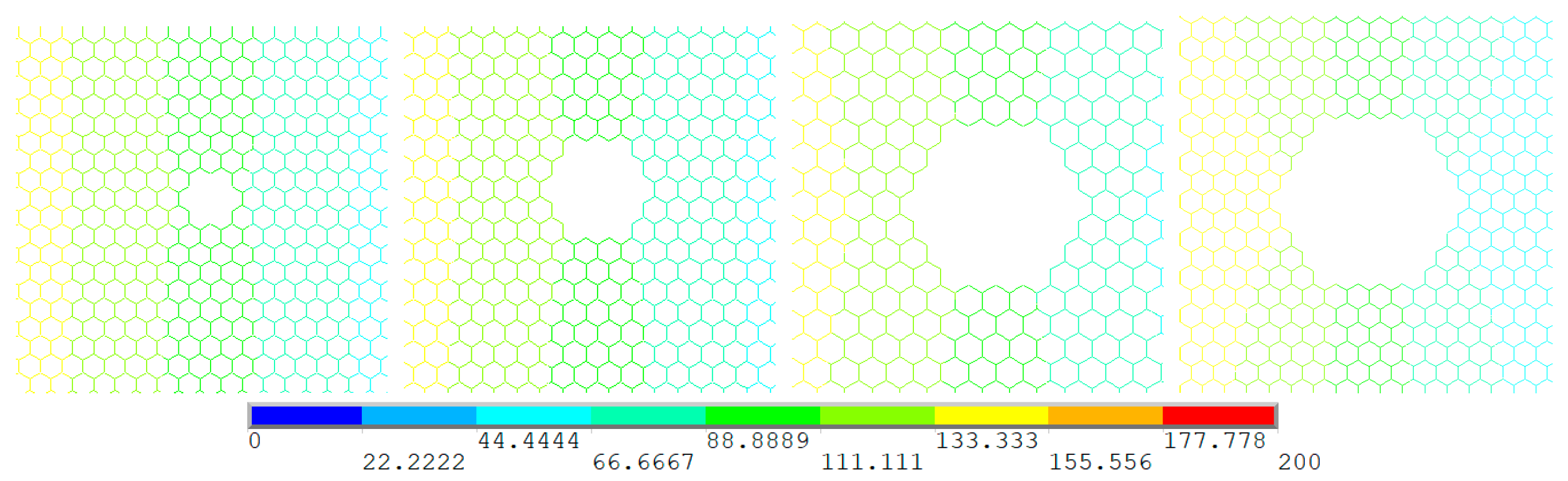
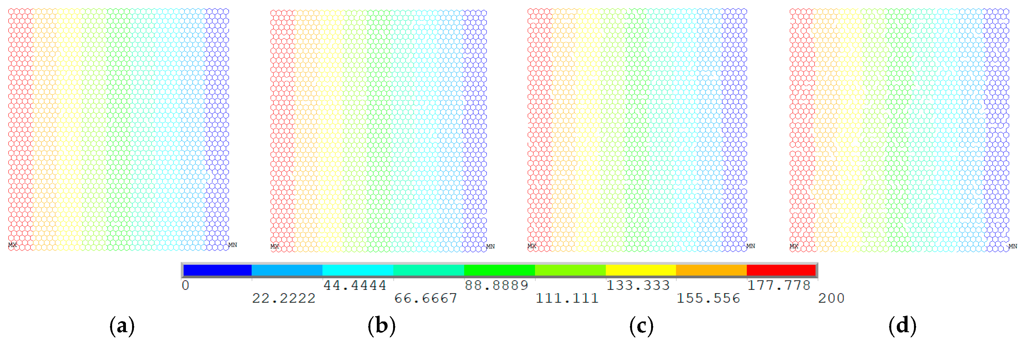
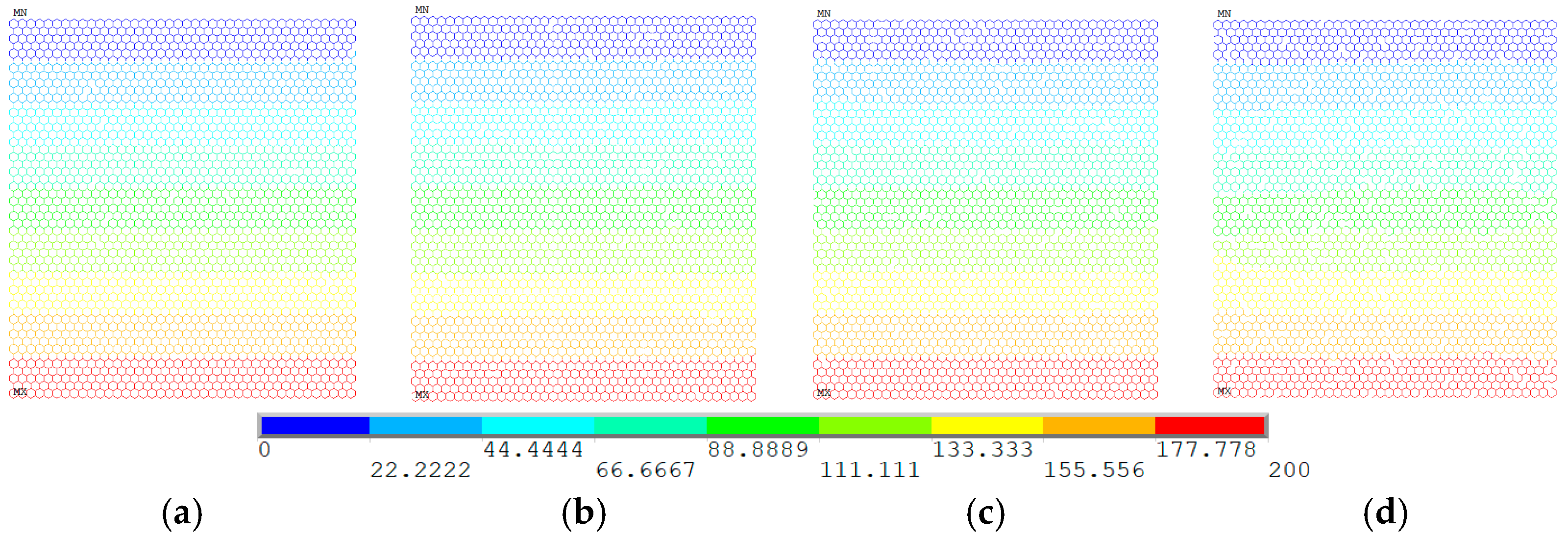
  • The center concentrated vacancy defects evidently destroyed the regularity and band characteristic of the temperature field in the steady-state thermal conduction. Moreover, the impacts of periodic and random distributed vacancy defects in temperature field of graphene is not convenient to track.
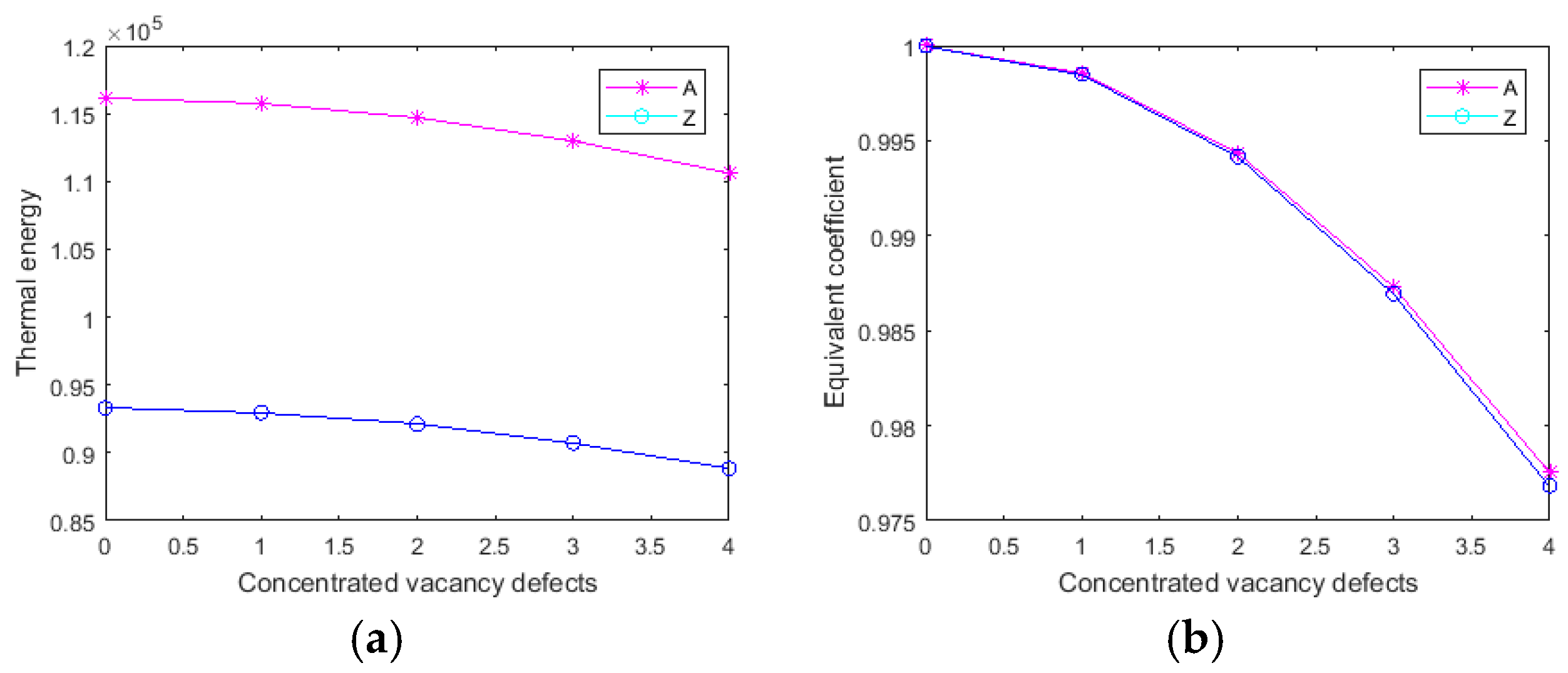
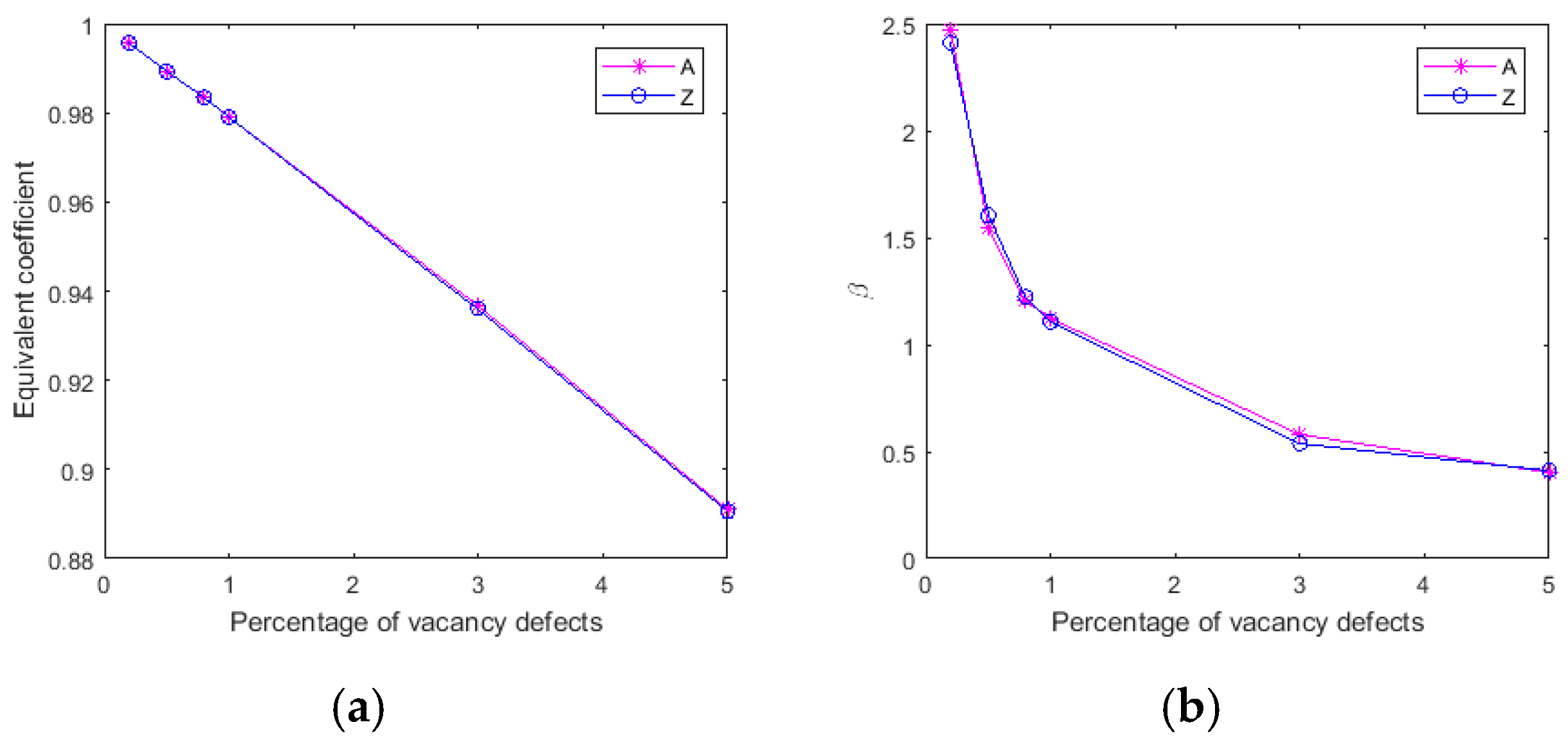
  • The graphene with periodic vacancy defects is sensitive to boundary conditions. The graphene with its heat source in armchair edges has a strengthening effect in the equivalent coefficient of thermal conductivity when periodic vacancy defects is distributed in the first mode. However, graphene with its heat source in zigzag edges is more robust to defend the reduction of the equivalent coefficient of thermal conductivity in the development of periodic vacancy defects. On the contrary, center concentrated and randomly distributed vacancy defects have a consistent equivalent coefficient of thermal conductivity under two boundary conditions.
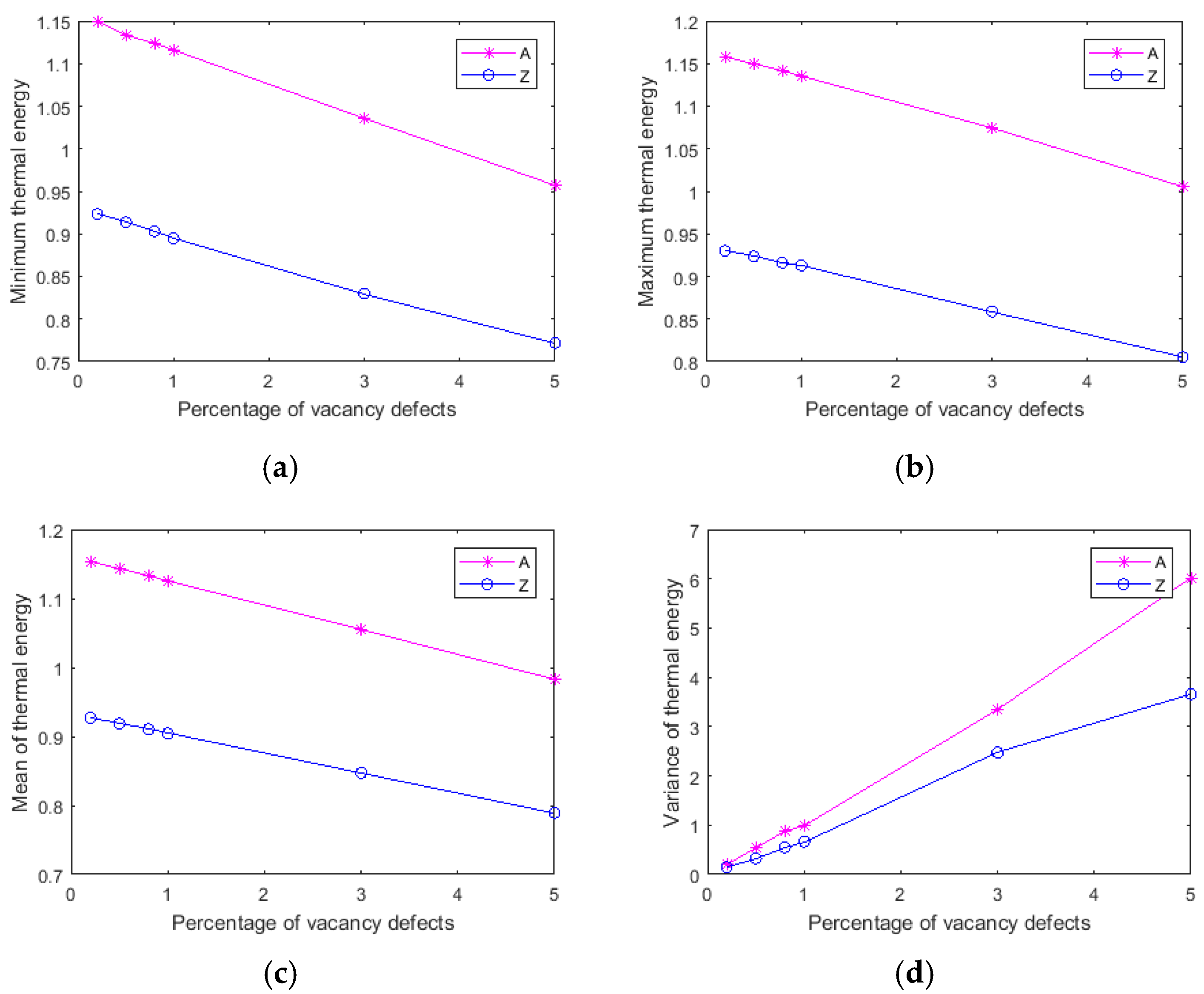
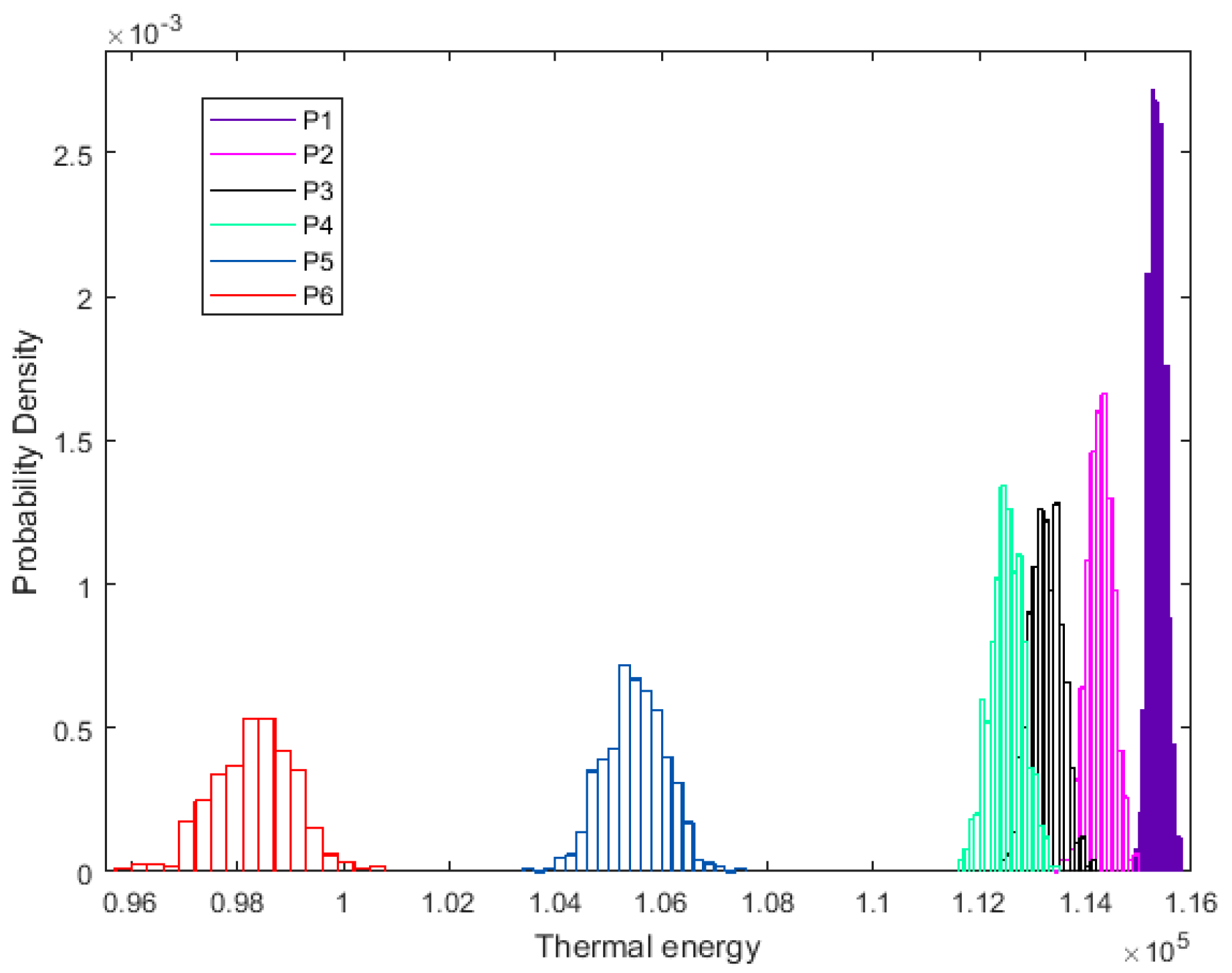
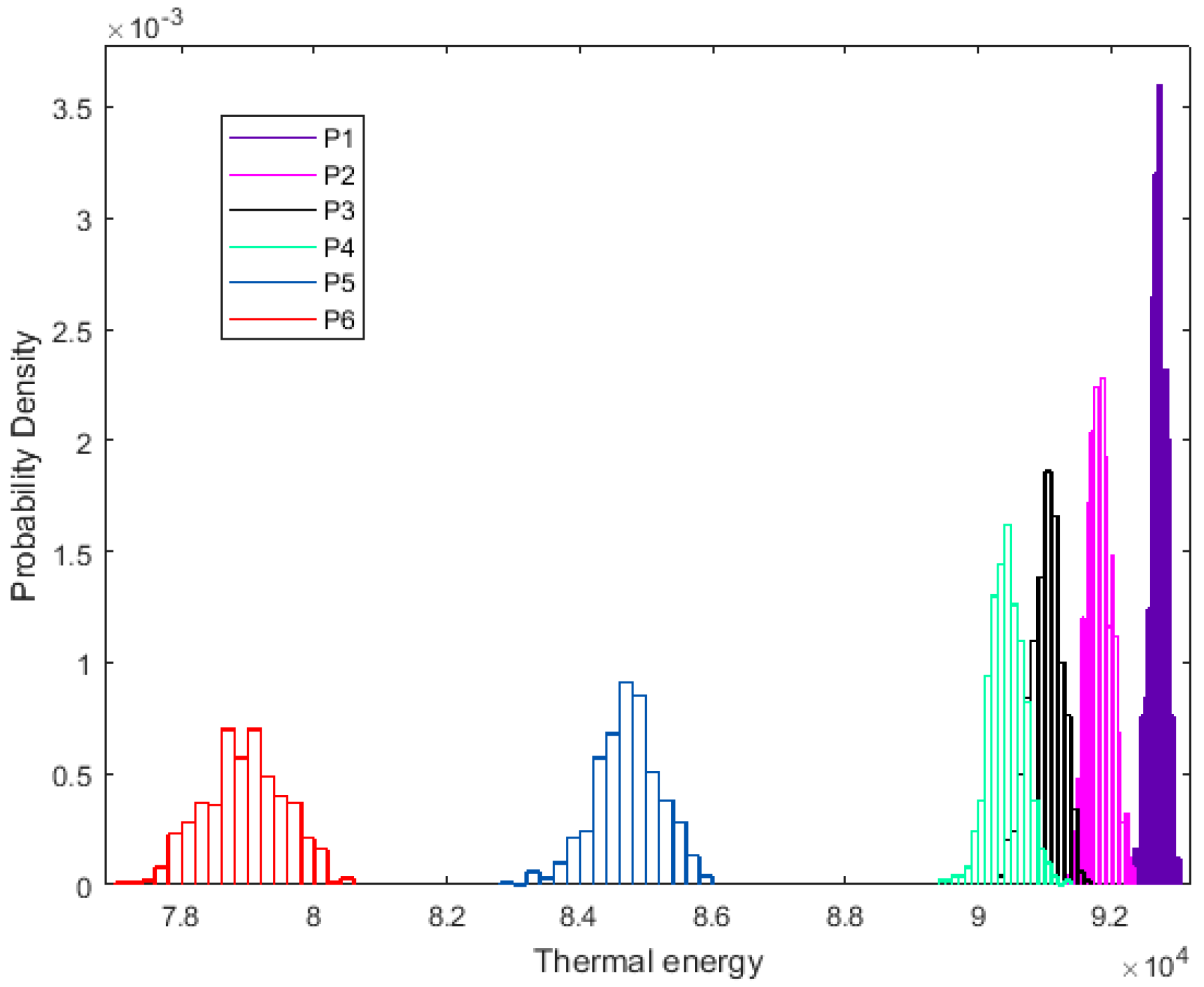
  • Furthermore, the amount and randomness of the vacancy defects are more important than the chirality in stochastically vacancy defected graphene. When Per equals to 0.2%, the reduction of thermal energy fluctuates from 0.3–1%, and from 13–17% when Per is 5%. The thermal energy has discrete range for certain quantity of random vacancy defects. The range of thermal energy is useful when reflecting on the amount of vacancy defects designed as a control switch in devices or instruments.
  • The robustness of graphene to resist the fluctuation owing to the randomness of vacancy defects declines sharply when Per is less than 1%. The variance caused by random dispersion of vacancy defects is amplified, according to the increment of Per.
  • Different than the center concentrated and periodic vacancy defects, the minimum, maximum, and mean values of thermal energy in graphene with random vacancy defects have a linear decreased tendency with the increase of vacancy amounts.

5. Data Availability Statement

The original data used to support the findings of this study are available from the corresponding author upon request.

Author Contributions

L.S accomplished the major work; L.C. came up with the main idea and performed the numerical analysis; J.S. accomplished the main writing for the research; and E.S.d.C. provided the mathematical and theoretical support for the research.

Funding

This research is supported by the National Natural Science Foundation of China (Grant No. 11602114).

Conflicts of Interest

The authors declare no conflict of interest.

References

  1. Kim, P.; Shi, L.; Majumdar, A.; Mc Euen, P.L.C. Thermal Transport Measurements of Individual Multiwalled Nanotubes. Phys. Rev. Lett. 2001, 87, 215502–215504. [Google Scholar] [CrossRef] [PubMed]
  2. Pop, E.; Mann, D.; Wang, Q.; Goodson, K.; Dai, H. Thermal conductance of an individual single-wall carbon nanotube above room temperature. Nano Lett. 2006, 6, 96–100. [Google Scholar] [CrossRef] [PubMed]
  3. Novoselov, K.S.; Geim, A.K.; Morozov, S.V.; Jiang, D.; Zhang, Y.; Dubonos, S.V.; Grigorieva, I.V.; Firsov, A.A. Electric field effect in atomically thin carbon films. Science 2004, 306, 666–669. [Google Scholar] [CrossRef] [PubMed]
  4. Geim, A.K.; Novoselov, K.S. The rise of graphene. Nanosci. Technol. 2009, 6, 11–19. [Google Scholar] [CrossRef]
  5. Novoselov, K.S.; Geim, A.K.; Morozov, S.V.; Jiang, D.; Katsnelson, M.I.; Grigorieva, I.V.; Dubonos, S.V.; Firsov, A.A. Two-dimensional gas of massless Dirac fermions in graphene. Nature 2005, 438, 197–200. [Google Scholar] [CrossRef] [PubMed]
  6. Zhang, Y.B.; Tan, Y.W.; Stormer, H.L.; Kim, P. Experimental observation of the quantum Hall effect and Berry’s phase in graphene. Nature 2005, 438, 201–204. [Google Scholar] [CrossRef]
  7. Balandin, A.A. Better computing through CPU cooling. IEEE Spectrum. 2009, 29, 33. [Google Scholar]
  8. Balandin, A.A.; Ghosh, S.; Bao, W.; Calizo, I.; Teweldebrhan, D.; Miao, F.; Lau, C.N. Superior thermal conductivity of single layer graphene. Nano Lett. 2008, 8, 902–907. [Google Scholar] [CrossRef]
  9. Ghosh, S.; Nika, D.L.; Pokatilov, E.P.; Balandin, A.A. Heat conduction in graphene: Experimental study and theoretical interpretation. New J. Phys. 2009, 11, 1–18. [Google Scholar] [CrossRef]
  10. Ghosh, S.; Bao, W.; Nika, D.L.; Subrina, S.; Pokatilov, E.P.; Lau, C.N.; Balandin, A.A. Dimensional crossover of thermal transport in few-layer graphene. Nat. Mater. 2010, 9, 555–558. [Google Scholar] [CrossRef]
  11. Ghosh, S.; Calizo, I.; Teweldebrhan, D.; Pokatilov, E.P.; Nika, D.L.; Balandin, A.A.; Bao, W.; Miao, F.; Lau, C.N. Extremely high thermal conductivity in graphene: Prospects for thermal management application in nanoelectronic circuits. Appl. Phys. Lett. 2008, 92, 151911. [Google Scholar] [CrossRef]
  12. Cai, W.; Moore, A.L.; Zhu, Y.; Li, X.; Chen, S.; Shi, L.; Ruoff, R.S. Thermal transport in suspended and supported monolayer graphene grown by chemical vapor deposition. Nano Lett. 2010, 10, 1645–1651. [Google Scholar] [CrossRef] [PubMed]
  13. Faugeras, C.; Faugeras, B.; Orlita, M.; Potemski, M.; Nair, R.R.; Geim, A.K. Thermal Conductivity of graphene in Corbino membrane geometry. ACS Nano 2010, 4, 1889–1892. [Google Scholar] [CrossRef] [PubMed]
  14. Jauregui, L.A.; Yue, Y.; Sidorov, A.N.; Hu, J.; Yu, Q.; Lopez, G.; Jalilian, R.; Benjamin, D.K.; Delk, D.A.; Wu, W.; et al. Thermal transport in graphene nanostructures: Experiments and simulations. ECS Trans. 2010, 28, 73–83. [Google Scholar]
  15. Saito, K.; Dhar, A. Heat conduction in a three dimensional anharmonic crystal. Phys. Rev. Lett. 2010, 104, 040601. [Google Scholar] [CrossRef] [PubMed]
  16. Lippi, A.; Livi, R. Heat conduction in two-dimensional nonlinear lattices. J. Stat. Phys. 2010, 100, 1147–1172. [Google Scholar] [CrossRef]
  17. Yang, L. Finite heat conductance in a 2d disorder lattice. Phys. Rev. Lett. 2002, 88, 094301. [Google Scholar] [CrossRef]
  18. Dhar, A. Heat conduction in the disordered harmonic chain revisited. Phys. Rev. Lett. 2001, 86, 5882–5885. [Google Scholar] [CrossRef]
  19. Klemens, P.G. Theory of the A-plane thermal conductivity of graphite. J. Wide Bandgap Mater. 2000, 7, 332–339. [Google Scholar] [CrossRef]
  20. Klemens, P.G.; Pedraza, D.F. Thermal conductivity of graphite in basal plane. Carbon 1994, 32, 735–741. [Google Scholar] [CrossRef]
  21. Nika, D.L.; Pokatilov, E.P.; Askerov, A.S.; Balandin, A.A. Phonon thermal conduction in graphene: Role of Umklapp and edge roughness scattering. Phys. Rev. B 2009, 79, 155413. [Google Scholar] [CrossRef] [Green Version]
  22. Berber, S.; Kwon, Y.-K.; Tomanek, D. Unusually high thermal conductivity if carbon nanotubes. Phys. Rev. Lett. 2000, 84, 4613–4616. [Google Scholar] [CrossRef] [PubMed]
  23. Lindsay, L.; Broido, D.A.; Mingo, N. Flexural phonons and thermal transport in graphene. Phys. Rev. B 2010, 82, 115427. [Google Scholar] [CrossRef]
  24. Munoz, E.; Lu, J.; Yakobson, B.I. Ballistic thermal conductance of Graphene ribbons. Nano Lett. 2010, 10, 1652–1656. [Google Scholar] [CrossRef] [PubMed]
  25. Savin, A.V.; Kivshar, Y.S.; Hu, B. Suppression of thermal conductivity in graphene nanoribbons with rough edges. Phys. Rev. B 2010, 82, 195422. [Google Scholar] [CrossRef]
  26. Huang, Z.; Fisher, T.S.; Murthy, J.Y. Simulation of phonon transmission through graphene and graphene nanoribbons with a green’s function method. J. Appl. Phys. 2010, 108, 094319. [Google Scholar] [CrossRef]
  27. Hu, J.; Ruan, X.; Chen, Y.P. Thermal conductivity and thermal rectification in graphene nanoribbons: A molecular dynamic study. Nano Lett. 2009, 9, 2730–2735. [Google Scholar] [CrossRef]
  28. Guo, Z.; Zhang, D.; Gong, X.-G. Thermal Conductivity of graphene nanoribbons. Appl. Phys. Lett. 2009, 95, 163103. [Google Scholar] [CrossRef]
  29. Evans, W.J.; Hu, L.; Keblinsky, P. Thermal conductivity of graphene ribbons from equilibrium molecular dynamics: Effect of ribbon width, edge roughness, and hydrogen termination. Appl. Phys. Lett. 2010, 96, 203112. [Google Scholar] [CrossRef]
  30. Aksamija, Z.; Knezevic, I. Lattice thermal conductivity of graphene nanoribbons: Anisotropy and edge roughness scattering. Appl. Phys. Lett. 2011, 98, 141919. [Google Scholar] [CrossRef] [Green Version]
  31. Lindsay, L.; Broido, D.A.; Mingo, N. Diameter dependence of carbon nanotube thermal conductivity and extension to the graphene limit. Phys. Rev. B 2010, 82, 161402. [Google Scholar] [CrossRef]
  32. Woodcraft, A.L.; Barucci, M.; Hastings, P.R.; Lolli, L.; Martelli, V.; Risegari, L.; Ventura, G. Thermal conductivity measurements of pitch-bonded at millikelvin temperatures: Finding a replacement for AGOT graphite. Cryogenics 2009, 49, 159–164. [Google Scholar] [CrossRef]
  33. Jang, W.; Chen, Z.; Bao, W.; Lau, C.N.; Dames, C. Thickness-dependent thermal conductivity of encased graphene and ultrathin graphite. Nano Lett. 2010, 10, 3909–3913. [Google Scholar] [CrossRef] [PubMed]
  34. Chen, S.; Moore, A.L.; Cai, W.; Suk, J.W.; An, J.; Mishra, C.; Amos, C.; Magnuson, C.W.; Kang, J.; Shi, L.; et al. Raman measurement of thermal transport in suspended monolayer graphene of variable sizes in vacuum and gaseous environments. ACS Nano 2011, 5, 321–328. [Google Scholar] [CrossRef]
  35. Lee, J.U.; Yoon, D.; Kim, H.; Lee, S.W.; Cheong, H. Thermal Conductivity of suspended pristine graphene measured by raman spectroscopy. Phys. Rev. B 2011, 83, 081419. [Google Scholar] [CrossRef]
  36. Nika, D.L.; Ghosh, S.; Pokatilov, E.P.; Balandin, A.A. Lattice thermal conductivity of graphene flakes: Comparison and bulk graphite. Appl. Phys. Lett. 2009, 94, 203103. [Google Scholar] [CrossRef]
  37. Mak, K.F.; Shan, J.; Heinz, T.F. Seeing many-body effects in single and few layer graphene: Observation of two-dimensional saddle point excitons. Phys. Rev. Lett. 2011, 106, 046401. [Google Scholar] [CrossRef]
  38. Bullen, A.J.; O’Hara, K.E.; Cahill, D.G.; Monteiro, O.; Von Keudell, A. Thermal conductivity of amorphous carbon thin films. J. Appl. Phys. 2000, 88, 6317–6320. [Google Scholar] [CrossRef] [Green Version]
  39. Chen, G.; Hui, P.; Xu, S. Thermal conduction in metalized tetrahedral amorphous carbon ta-c films on silicon. Thin Solid Films 2000, 366, 95–99. [Google Scholar] [CrossRef]
  40. Shamsa, M.; Liu, W.L.; Balandin, A.A.; Casiraghi, C.; Milne, W.I.; Ferrari, A.C. Thermal conductivity of diamond like carbon films. Appl. Phys. Lett. 2006, 89, 161921. [Google Scholar] [CrossRef]
  41. Balandin, A.A.; Shamsa, M.; Liu, W.L.; Casiraghi, C.; Ferrari, A.C. Thermal conductivity of ultrathin tetrahedral amorphous carbon. Appl. Phys. Lett. 2008, 93, 043115. [Google Scholar] [CrossRef]
  42. Huang, Y.; Wu, J.; Hwang, K.C. Thickness of graphene and single-wall carbon nanotubes. Phys. Rev. B 2006, 74, 245413. [Google Scholar] [CrossRef]
  43. Odegard, G.M.; Gates, T.S.; Nicholson, L.M.; Wise, K.E. Continuum model for the vibration of multilayered graphene sheets. Compos. Sci. Technol. 2002, 62, 1869. [Google Scholar] [CrossRef]
  44. Murali, R.; Yang, Y.; Brenner, K.; Beck, T.; Meindl, J.D. Breakdown current density of graphene nanoribbons. Appl. Phys. Lett. 2009, 94, 243114. [Google Scholar] [CrossRef] [Green Version]
  45. Seol, J.H.; Jo, I.; Moore, A.L.; Lindsay, L.; Aitken, Z.H.; Pettes, M.T.; Li, X.; Yao, Z.; Huang, R.; Broido, D.; et al. Two-dimensional phonon transport in supported graphene. Science 2010, 328, 213–216. [Google Scholar] [CrossRef] [PubMed]
  46. Chu, L.; Shi, J.; Souza de Cursi, E. Vibration Analysis of Vacancy Defected Graphene Sheets by Monte Carlo Based Finite Element Method. Nanomaterials 2018, 87, 489. [Google Scholar] [CrossRef]
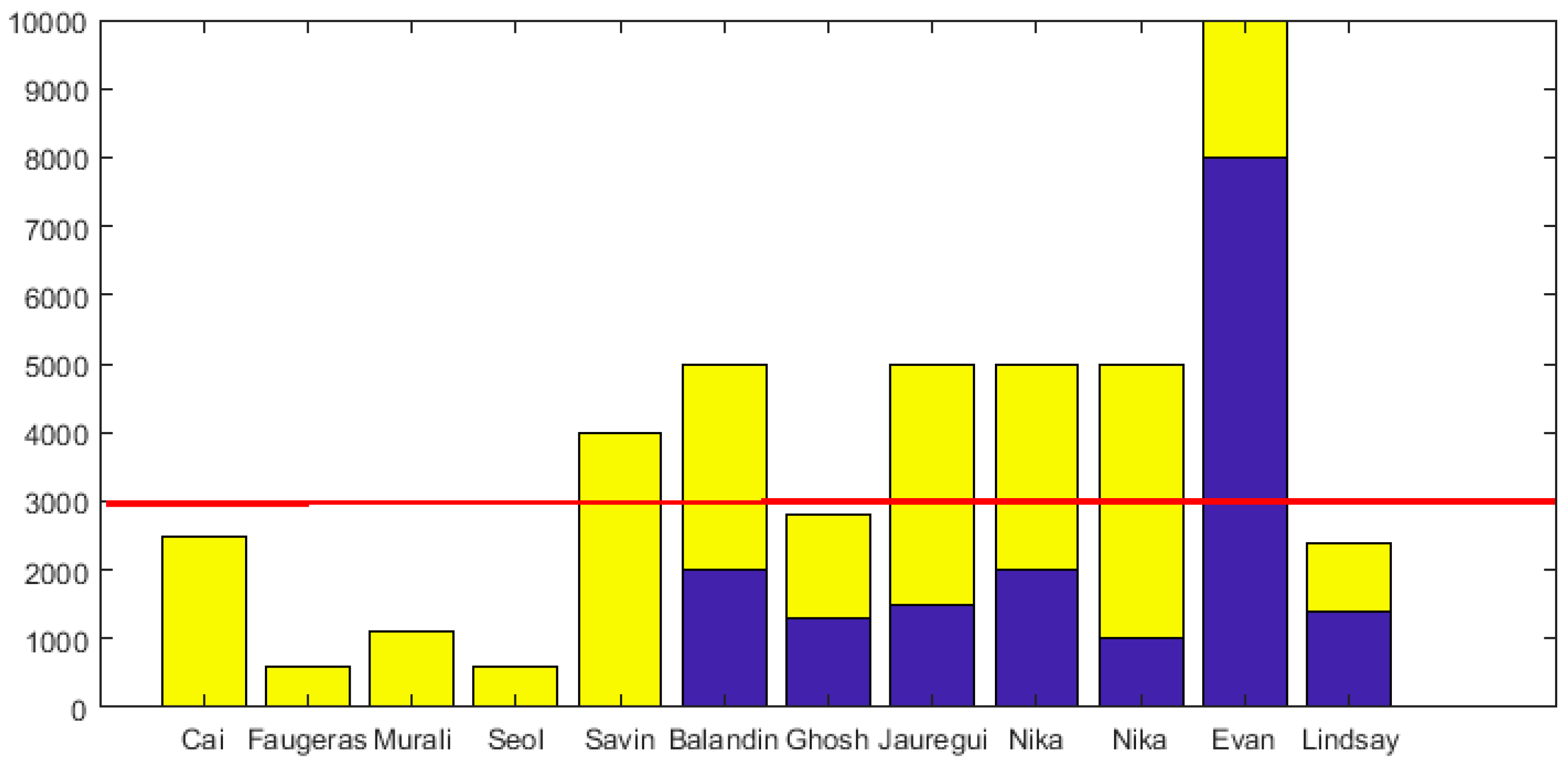
Figure 1. Thermal conductivity of graphene (unit: W/mK).
Applsci 09 02363 g001
Figure 2. Finite element model (FEM) for graphene lattice.
Applsci 09 02363 g002
Figure 3. Finite element model of pristine graphene for the thermal conduction. (a,b) is its heat source in the armchair and zigzag edge, respectively.
Applsci 09 02363 g003
Figure 4. Graphene with vacancy defects. (ac) are for center concentrated, periodic, and random distributed vacancy defects, respectively.
Applsci 09 02363 g004
Figure 5. Center concentrated vacancy defects. The size of center concentrated vacancy defects is gradually amplified from (ad).
Applsci 09 02363 g005
Figure 6. The results of graphene with center concentrated vacancy defects (A—heat source in armchair edges, Z—heat source in zigzag edges, and (a) is for the thermal energy, (b) is for the equivalent coefficient, unit for thermal energy is J).
Applsci 09 02363 g006
Figure 7. Temperatures in the local region around the center concentrated vacancy with its heat source in armchair edges.
Applsci 09 02363 g007
Figure 8. Temperatures in the local region around the center concentrated vacancy with its heat source in zigzag edges.
Applsci 09 02363 g008
Figure 9. Periodic dispersion vacancy defects. (ad) for first-fourth mode of periodic vacancy defects.
Applsci 09 02363 g009
Figure 10. The results of graphene with periodic vacancy defects. A—heat source in armchair edge, Z—heat source in zigzag edge. And (a) is for the thermal energy, (b) is for the equivalent coefficient, unit for thermal energy is J.
Applsci 09 02363 g010
Figure 11. Temperatures of graphene with its heat source in armchair edges (The four figures are for the graphene sheets with generally increasing periodic vacancy defects).
Applsci 09 02363 g011
Figure 12. Temperatures of graphene with its heat source in zigzag edges (The four figures are for the graphene sheets with generally increasing periodic vacancy defects).
Applsci 09 02363 g012
Figure 13. The statistical results of graphene with random distributed vacancy defects (the unit for thermal energy is 105 J; (ad) are the minimum, maximum, mean, and variance values of the thermal energy, respectively.
Applsci 09 02363 g013
Figure 14. The histogram of probability density distribution of thermal energy in graphene with its heat source in armchair edges (P1–P6 represents the percentage of vacancy as 0.2%, 0.5%, 0.8%, 1%, 3%, and 5%, respectively, and the unit for thermal energy is J).
Applsci 09 02363 g014
Figure 15. The histogram of probability density distribution of thermal energy in graphene with its heat source in zigzag edges (P1–P6 represents the percentage of vacancy as 0.2%, 0.5%, 0.8%, 1%, 3%, and 5%, respectively, and the unit for thermal energy is J).
Applsci 09 02363 g015
Figure 16. Ratio of thermal energy reduction (A-1 and A-2 are for minimum and maximum thermal energy in graphene with its heat source in armchair edges, respectively; Z-1 and Z-2 for minimum and maximum thermal energy in graphene with its heat source in zigzag edges, respectively).
Applsci 09 02363 g016
Figure 17. The robustness of graphene with random distributed vacancy defects. (a) is for the equivalent coefficient, (b) is for β .
Applsci 09 02363 g017
Figure 18. Temperature results of random vacancy defected graphene with its heat source in armchair edges (the percentages of vacancy defects in (ad) are 0.2%, 0.5%, 1%, and 3%, respectively).
Applsci 09 02363 g018
Figure 19. Temperature results of random vacancy defected graphene with its heat source in zigzag edges (the percentages of vacancy defects in (ad) are 0.2%, 0.5%, 1%, and 3%, respectively).
Applsci 09 02363 g019
Table 1. Thermal conductivity of graphene in reference.
ReferenceK (W/mK)Method
Balandin [8]2000–5000RO, exfoliated
Ghosh [10]1300–2800RO, exfoliated
Jauregui [14]1500–5000RO, CVD
Cai [12]2500RO, CVD
Faugeras [13]600RO, exfoliated
Murali [44]1100Electrical self-heating, exfoliated
Seol [45]600Electrical, exfoliated
Savin [25]4000Ballistic, width dependence
Nika [21]2000–5000VFF, BTE, width dependence
Nika [36]1000–5000RTA, size dependence
Evan [29]8000–10000MD, square graphene sheet
Lindsay [31]1400–2400BTE, length dependence
Raman optothermal—RO, chemical vapor deposition—CVD, VFF—valence force field, BTE—Boltzmann transport equation, RTA—relaxation time approximation, MD—molecular dynamics.
Table 2. Statistical thermal energy results for random distributed vacancy defects (unit: ×105 J).
TypePer (%)Minimum MaximumMeanVariance
A0.21.14941.15771.15350.2181
0.51.13351.14961.14280.5465
0.81.12431.14191.13260.8798
11.11631.13491.12521.0048
31.03491.07521.05503.3332
50.95711.00630.98316.0168
Z0.20.92320.93010.92710.1480
0.50.91350.92340.91840.3278
0.80.90320.91610.91020.5540
10.89480.91300.90430.6667
30.83000.85890.84722.4754
50.77180.80500.78943.6630

