1. Introduction
5G networks are expected to provide a wide variety of services to individual users and industry customers who may have different quality of service (QoS) requirements. The explosive data traffic demand in 5G has stressed the need for the network capacity increase. Thus, 5G should be more flexible and scalable enough to meet a variety of requirements of the traffic. However, traditional network upgrade methods for increasing the network capacity such as vertical and horizontal scaling create excessive operating and capital expenses of network operators. The concept of network slicing through resource sharing has been presented as a promising solution to achieve efficient and affordable 5G. Network slicing divides a single physical network into multiple virtual networks to be configured to provide specific QoS as required by different applications and traffic classes. From the network management point of view, the mechanism for resource allocation across slices is the major research direction for network slicing and enables each slice’s own set of allocated resources to be separately operated and maintained.
Network slicing provides new business opportunities for service providers and vertical industries, including healthcare, IoT, smart cities, and mobile broadband services. Since network slices will be used by traffic engineering businesses, network slicing is a matter of business and economic model as well as a simple resource allocation mechanism. Entities involved in the network slicing business can be roughly categorized into slice providers and slice tenants. The owner of each network slice is known as a slice tenant [
1]. The slice provider provides the customized network to the slice tenants [
2]. Each entity independently pursues a profit-earning business model. The slice tenants have the discretion to decide how much amount of resource should be purchased according to the traffic and market conditions. The slice provider can establish a service level agreement (SLA) contract according to resource requests from slice tenants. In addition, users, who consume services offered by each tenant, pay tenants a fee for using the services.
Despite the resource sharing concept, which is a key idea of network slicing, has recently attracted considerable attention, an efficient use of resources is still a challenge. In legacy networks, every tenant pays a fixed and roughly estimated monthly or annual fee for shared resources according to a contract signed with a provider in an exclusive and excessive manner [
3]. The 3rd Generation Partnership Project (3GPP) suggests that static resource allocation based on fixed network sharing can be one of the approaches for resource management in network slicing. However, such a static allocation mechanism may lead to low efficiency. For example, suppose that an amount of bandwidth enough to support the peak traffic demand is statically allocated to a network slice. In this case, the bandwidth utilization will be low on average due to continuous fluctuations in the network demand, even leading to a very high tenant’s cost. Obviously, exclusive and excessive resource allocation, which cannot adapt to the change of network demand, is not a cost-effective method.
A dynamic resource trading mechanism can be a solution to the inefficient resource allocation. With dynamic trading of shared resources, a network operator can allocate the necessary resources as traffic changes. However, it is difficult to negotiate and optimize resource allocation, because the resource is not managed by a single management entity, and several business entities independently participate in resource trading for their own benefit. This dynamic trading involves a very high computational cost and can make it impractical for real-scenarios. As a solution, Q-learning can be a reasonable approach; it can choose an optimal action in real-time without considering the future information at upcoming slots, which may represent a definite advantage in real-world scenarios.
On the 5G standardization front, various approaches to resource management in network slicing are currently specified by the 3GPP. The slice tenant and provider are the entities that provide various services; thus, they should negotiate the resource according to the information such as the type of service and traffic fluctuations. In this paper, we propose a resource management mechanism based on variations of the traffic mix using Q-learning algorithm. Our approach is based on the ability of tenants to manage resource allocation and negotiate their resource with the provider. Since we focus on resource management from each tenant’s point of view, the Q-learning algorithm operates on each tenant’s resource management controller. A tenant has two business interfaces: one interface toward the provider, and the other toward the end-user. The former interface is used for acquiring network resources upon the requirements and paying for the resources to the provider. In other words, each independent tenant trades resources with the provider, and there is no direct resource transaction between the tenants. The tenant interacts with end-users using the latter interface to provide the resources to them. Under such a Q-learning-based dynamic resource trading environment, each tenant exhibits a strategic behavior to maximize its own profit. Meanwhile, since the tenants are independent business entities, they want to purchase as much amount of resource as they need, and, in this case, the physical resource may become scarce. Therefore, the provider manages the limited resource by increasing the resource price as the resource demand increases. This basic knowledge of the market is that the price increases if the demand increases, and this mechanism keeps the trading market in balance [
4]. Our contributions are summarized as follows.
We model a network slicing resource trading process between the slice provider and multiple tenants in a network slicing environment using a Markov Decision Process (MDP).
We propose taking a ratio of the number of inelastic flows to the total number of flows in each network slice as an MDP state parameter to characterize different QoS satisfaction properties of each slice to the change of slice resource allocation.
We propose a Q-learning-based dynamic resource management strategy to maximize tenant’s profit while satisfying QoS of end-users in each slice from each tenant’s point of view.
The rest of the paper is organized as follows. In
Section 2, we briefly review the related work on resource management systems and business models in network slicing. In
Section 3, we describe the service model and resource trading model for network slicing. In
Section 4, we outline the design of the proposed resource management system using an MDP. In
Section 5, we propose a dynamic resource adjustment algorithm based on the Q-learning approach. We present the performance evaluation results in
Section 6. Finally, we conclude this paper in
Section 7.
2. Related Work
The topic of network slicing has received substantial attention among the research community. The end-to-end network slicing allocates slice components spread across the entire network to the tenants to satisfy the diverse requirements with flexibility and scalability [
5]. From the current technology’s point of view, although network slicing is still a theoretical step, many researchers are looking forward to making a commercial product out of the network slicing concept for 5G systems because of the flexibility and scalability provided by network slicing. In fact, business opportunities of network slicing paradigm can promote an economic advantage for 5G. In [
6], Habiba and Hossain conducted a survey of the economic aspects of network slicing virtualization in terms of network resource and pricing based on various auction mechanisms. They presented the fundamentals of auction theory in designing the business model and simultaneously attempted to optimize resource utilization and profit using a pricing rule. The auction theory is able to model interactions among the provider and multiple tenants. In [
7], Luong et al. reviewed resource pricing approaches for efficient resource management to maximize the benefits of the provider and tenants. They emphasized that an efficient mechanism of resource allocation is required for the high resource utilization of the provider and QoS for end-users of tenants.
There has been a significant amount of research work on the management and orchestration of network slicing. In [
8], Alforabi et al. comprehensively summarized principal concepts, enabling technologies and solutions as well as the current standardization efforts such as the software-defined networking (SDN) and network function virtualization (NFV). By presenting relevant research, they described how end-to-end network slicing can be achieved by designing, architecting, deploying, and managing network components in 5G networks. An important issue of network slicing is the resource allocation to satisfy a number of heterogeneous service requirements by taking the tenant’s point of view. Under such a resource allocation model, every tenant has the ability to allocate network resources to their own slice according to their strategic behavior. In [
9,
10], Caballero et al. focused on resource allocation based on a game-theoretical model for tenants’ strategic behavior and analyzed parameters to reduce cost while maintaining the QoS. The Fisher market mechanism has been used to share the resources of each tenant in a fair manner according to different requirements of end-users who are served by each tenant. The tenants indicate their preferences to the infrastructure and then receive resources of the base station according to their preferences. On the other hand, there is a strategy of the resource allocation and admission control focusing on how the mobile network operator (MNO) adjust slice parameters to maximize the overall revenue. When a tenant issues a service request to create a new slice, the MNO considers the admission of the slice. If MNO determines approval of the request, a slice is created and granted to the tenant. In [
11], Bega et al. proposed a mechanism that MNO has the authority of admission control of tenants to maximize the revenue of a network. In [
3], Han et al. proposed a genetic optimization for resource management across the slices using an MNO’s binary decision.
However, the majority of such studies have not considered dynamically changing resource requirements over time. Thus, most of their business models were quite simple in that a fixed and roughly estimated monthly or annual fee was paid for the resource sharing. The operation in such a framework can often incur unnecessary expenditure due to unused resources or resource scarcity. To address this issue, there are some studies that have considered resource trading in the context of network slicing. In [
12], Xie et al. proposed a dynamic resource pooling and trading mechanism in network virtualization using Stackelberg game to achieve more efficient utilization of network resources. In [
13,
14], Akguel et al. proposed an algorithm for trading resources among tenants. However, their approach involves a high computational cost that can make it impractical for real-scenarios. In contrast, we consider Q-learning-based approach to determine how much amount of resource a tenant needs to purchase in advance using only the current information while considering the future rewards at upcoming slots. This reinforcement learning based approach can solve the resource trading problem for network slicing with reasonably low complexity, and thus is applicable to real-world applications in practice.
4. Resource Trading System Using a Markov Decision Process
In this section, we outline the design of our dynamic resource trading system that aims at maximizing the profit of a slice tenant using an MDP. The MDP is defined by a 4-tuple as , where , , , and denote the state space, action space, reward function, and transition probability, respectively. In any state at time slot t, one of the available actions can be selected. After the selected action has been taken, the state may change to the next state with a state transition probability of . represents an immediate reward that can be obtained by taking action in state .
4.1. State Space
In our system, the tenant plays a role as an agent that interacts with the environment and exhibits strategic behavior to maximize its reward. The state space at time slot
t can be defined as
where
,
,
, and
are the flow ratio of the slice, total resource demand, current market price ratio, and time zone index of the current time slot, respectively. The information of these four state elements is considered to be known to the tenant at each time slot
t.
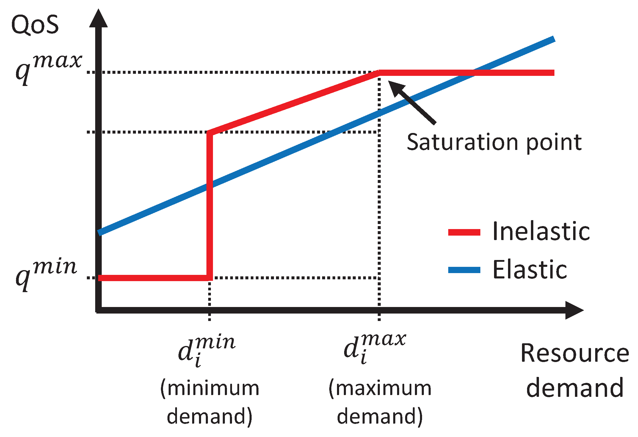
To characterize the type of services supported by each slice, we define the flow ratio, denoted as
, which is computed by dividing the number of inelastic flows by the total number of flows as follows:
where
I and
E denote the set of inelastic and elastic flows, respectively. We expect
to be used as a parameter to determine how much bandwidth the tenant purchases in advance. It is a very important approach for our dynamic resource trading system because the system will violate QoS and get a penalty if there is not enough immediate bandwidth. The effect of
on the system performance is analyzed in detail in
Section 6.
Let
be the sum of the minimum demands of all inelastic flows belonging to slice
n at time slot
t and
denote the sum of the average demands of all elastic flows served by slice
n at time slot
t, respectively, as follows:
Then, we can define the total resource demand at time slot
t, which is the sum of the minimum demands of all inelastic flows and average demands of all elastic flows, as follows:
If the total bandwidth demand exceeds the total purchased bandwidth at time slot t, i.e., , resource utilization is 1 because the used bandwidth cannot exceed the total purchased bandwidth.
The price ratio, denoted as , represents the ratio of the unit price of the bandwidth that tenants purchase from the provider to the unit price of the bandwidth that they sell to the end-user, i.e., . is included in the state since it highly affects the profit of the slice tenant. We assume that is determined by the provider according to the amount of the total resource remained in the physical network. For example, if the amount of remaining resource in the physical network is decreased, the provider increases . This implies that can play an important role in the resource balancing in the physical network through regulating the amount of resource being purchased by adjusting .
Time slot needs to be included in the state because the tenant may act differently at different time slots. As an effort to avoid a situation that the number of states goes infinitely high, we apply the concept of the time zone; i.e., we use the index of the time zone rather than the index of the actual time slot. Let
and
T denote the number of time zones in the slice and the lifetime of the slice, respectively. Then, the time zone index of the current time slot can be defined as follows:
4.2. Action Space
In a given state
, the tenant selects an action
from the set of possible actions defined as
where
represents the resource trading unit. For instance, if a positive/negative action is taken, the agent increases/decreases the amount of resource being bought from the provider.
means that the agent keeps maintaining the amount of resource. We define a possible action set
in the action space
A. In each trading interval
h,
is constrained by the amount of the allocated resource. For example, if a slice does not have enough resource to satisfy the requirements, i.e.,
, it certainly has to purchase more bandwidth, whereas if
, one more action,
, is also available. Otherwise, all actions are available. As a result,
can be determined as follows:
4.3. Reward Function
Let
denote the reward function that returns a reward indicating the profit of the tenant. When action
is taken at state
,
can be defined as
where
is the QoS-weight factor determining the importance of the QoS compared to the profit. In Equation (
11),
is an amount of bandwidth that violates QoS when the total resource demand
exceeds the achievable rate
at time slot
t (i.e.,
). In other words, if the amount of bandwidth is insufficient compared to the resource demand, the QoS of some flows may be violated. In this case, a penalty will be imposed by
. To let the system meet the QoS more strictly, we can increase
to impose a larger penalty for the QoS violations. Using the reward
, we define the total discounted reward
to take into account future rewards as follows:
where
is a discount factor weighting future rewards relative to current rewards. Our ultimate goal is to find an optimal policy that can maximize
. In the next section, a dynamic resource adjustment algorithm using Q-learning is proposed to find the optimal policy.
5. Dynamic Resource Adjustment Algorithm
Based on the model presented in the previous section, we propose a dynamic resource adjustment algorithm that aims at maximizing slice tenant’s profit by learning with the reward resulting from the previous action while satisfying the requirements of flows. Our adjustment algorithm is based on the Q-learning approach. Q-learning is one of the most widely used reinforcement learning techniques, which finds and selects an optimal action based on Q-function that defines state–action pairs. A Q-value represents the expected long-term reward of an agent under the assumption that it chooses the best actions from a specific state. First, the agent perceives the current states of the system and takes an action according to policy
defined as
where
is the Q-value, and the system keeps a memory for all state–action pairs. If the action
that has the maximum Q-value at the current state is selected by the policy, the reward is calculated according to Equation (
11), leading to updating the Q-value. If the agent infinitely visits all state–action pairs, Q-values converge to an optimal value.
However, always taking the best action with the maximum Q-value at every state (i.e., exploitation) may result in a wrong decision after the completion of learning. The agent should be exposed to as many states as possible to learn how to deal optimally with all of them. Thus, the algorithm also needs to explore all possible
options, including those that do not maximize the Q-value (i.e., exploration). The exploration strategy involves performing random actions to experience environmental changes to preclude from focusing on immediate rewards, whereas the exploitation strategy makes use of only what the agent knows already. We adopt the
-greedy method to establish the exploration and exploitation balance. It means that the agent exploits the action that minimizes the immediate reward
and explores random actions with a probability
. Therefore, the probability of selecting action
in state
under policy
, denoted as
, can be represented as
To maximize the overall reward of the agent, the algorithm constantly learns the characteristics of the system by exploring it and taking decisions many times. The action to be taken in the current state depends on the Q-value
. The learning process continuously updates Q-values until the system can take the best action for all states. The agent updates the action-value function according to the following rule:
where
denotes the learning rate that determines how fast the learning happens, whereas the discount factor
weighs the importance of future rewards in making the current decision. When
is small, it will take a long time for the algorithm to converge, whereas, with a large
, the algorithm might not converge. Setting
to a small value results in the Q-value being optimized by immediate rewards, whereas, with large
values, the algorithm heavily depends on future rewards. An appropriate selection of
and
can allow achieving effective control of the Q-learning process.
The pseudo-code of the proposed resource adjustment algorithm is shown in Algorithm 1. The algorithm maintains the Q-values that are being iteratively updated when new events happen. First, the parameters for Q-learning are initialized. In particular, the Q-values are initialized to zeros (Lines 1–2). At each time slot t, the agent monitors the states (i.e., the flow ratio of the slice, total resource demand, current market price ratio and time zone index) (Line 4). The possible action set considering the current resource state is determined for each trading interval (Line 6). An action with the highest Q-value or a random action with a probability of following the -greedy policy can be taken from (Line 7). Based on the selected action, the environment changes the state and provides the agent with a reward (Line 8). The algorithm calculates the Q-value using the learning rate (Line 9).
| Algorithm 1 Resource adjustment algorithm using Q-learning. |
- 1:
Initialize , and . - 2:
Initialize learning parameters , and - 3:
for each time slot t do - 4:
Monitor states - 5:
for each trading interval h do - 6:
Determine a possible action set by ( 10) - 7:
Select action from using policy derived from -greedy by ( 13) - 8:
Take action and observe and - 9:
Update by ( 15) - 10:
end for - 11:
and - 12:
end for
|
6. Performance Evaluation
This section describes the MATLAB simulation results to evaluate the performance and effectiveness of the proposed Q-learning-based resource adjustment algorithm.
6.1. Setup of the Simulation Environment
We implemented a network slicing simulation environment to simulate behaviors of a slice tenant and evaluate its profit and QoS. The tenant can trade resources according to the strategies defined in the simulation. Once the slice is created, the initial resource is allocated to the slice, and the slice has to keep the minimum resource (). We considered a scenario with 200 flows, where the ratio between inelastic and elastic flows is randomly chosen to be between 0 and 1. We set the number of time zones to 10 and the lifetime of the slice to 100 time slots. Unless otherwise stated, the unit buying price and unit selling price of the bandwidth were set to $40 and $200, respectively, and the QoS weight was set to . We assumed that requests for flow creation are issued following a Poisson process of rate , and every flow has a random lifetime that follows an exponential random variable of rate . The initial resource is first bundled into slices and then allocated to slices.
6.2. Q-Learning Algorithm Convergence
To demonstrate the effectiveness of our Q-learning algorithm, we observed the average reward of Q-learning with respect to trading episodes. The Q-values are stored in the Q-table and updated during the training process of the algorithm. The Q-table is initialized with zeros. We considered that the Q-learning algorithm is implemented by the tenant with and . To speed up the convergence rate, can be set closer to 1; however, a higher value of would lead to local optimization. We also employed the -greedy strategy to make sure that all state–action pairs are explored enough before converging to a particular action. Since the value of exploration was high at the beginning, we defined as a linear function of the episode. In other words, we set the initial value of to 1, and approached 0 as the episode number increased. This was only done for the first 50% of the episodes, whereas was 0 for the rest of the episodes. This was to ensure that every action was performed a sufficient number of times before converging to a particular action.
Figure 3 illustrates the convergence speed of the Q-learning algorithm with the average reward and standard deviation (red region) obtained per episode during the learning process. We assumed that the system had reached convergence when the mean of all Q-values did not change over time. It was observed that Q-values started from a low initial reward level but quickly converged to a competitive trading strategy with a satisfying reward performance within hundreds of episodes. This result shows that Q-values are successfully learned after a certain number of episodes and can achieve better resource trading than that without any prior training.
6.3. Competitiveness
To verify the competitiveness of our algorithm, we next evaluated the performance of our algorithm by comparing it with the following strategies:
Fixed-resource strategy allocates enough resources in an exclusive and excessive manner. This strategy is the most straightforward algorithm.
Half-of-demand strategy allocates resources equal to a half of the entire resource demand of the previous episode.
Previous-slot-demand strategy dynamically allocates resources corresponding to the resource demand of the previous time slot.
Among these strategies,
fixed resource and
half of demand are static resource allocation algorithms, whereas
previous demand and our Q-learning-based algorithm are dynamic trading strategies.
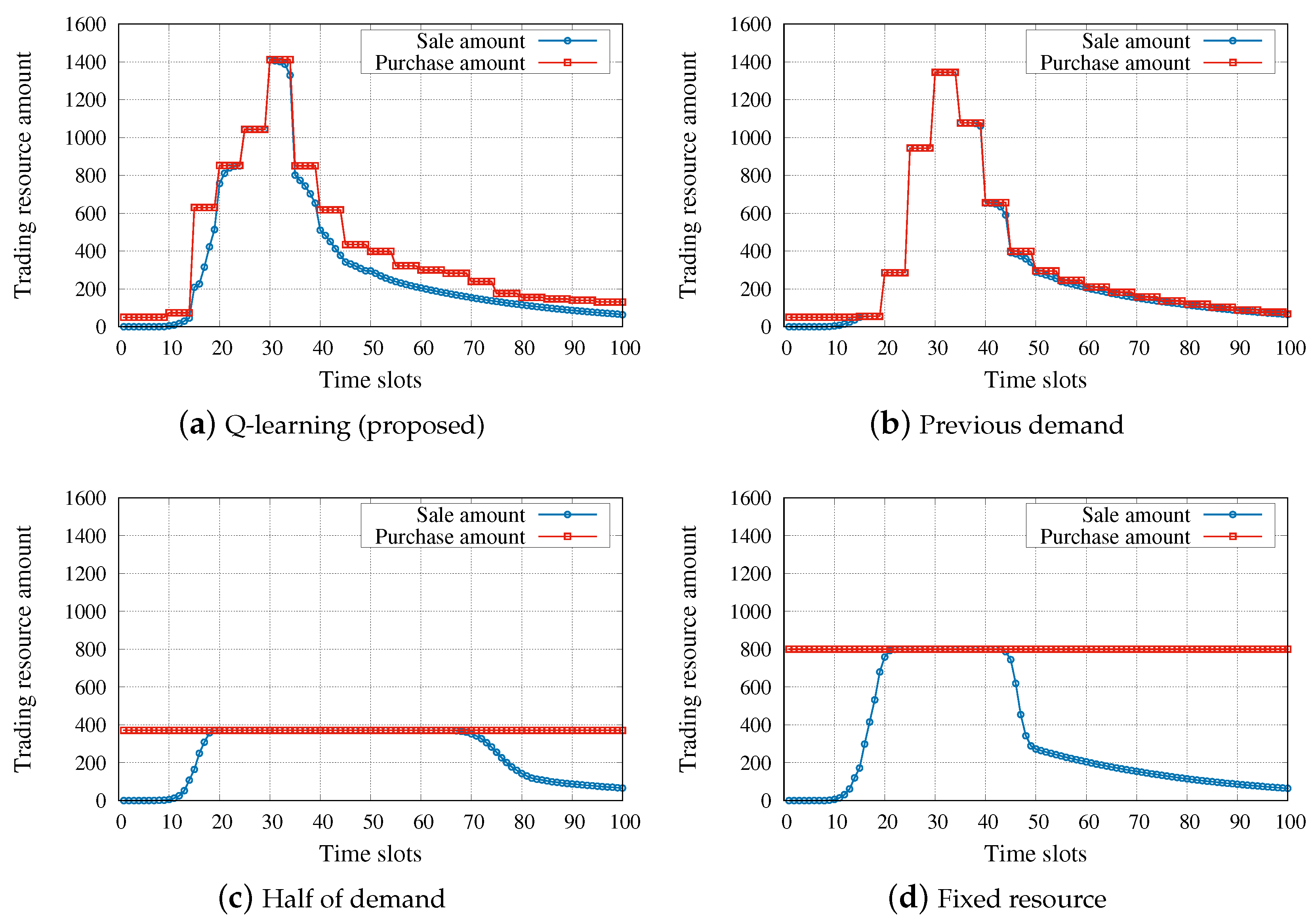
Figure 4 shows the purchase and sale amounts obtained by each of the strategies. The same simulation parameters were used in all four simulations as mentioned above, where the flow ratio was chosen randomly. In the static resource allocations, available resources are distributed among tenants based on a predefined algorithm regardless of current states of slices. Note that we set the fixed purchase amount of
fixed-resource method so that the QoS satisfaction rate is less than 0.01 (i.e.,
). As expected, the
fixed-resource method, which is the basic strategy of a legacy network, does not violate the QoS but results in a very low resource utilization. Although the
half-of-demand strategy tries to overcome the low resource utilization problem of the
fixed-resource strategy, the QoS can be violated to a greater extent when increasing the proportion of inelastic flows in the slice. In the dynamic resource adjustment algorithms, the slices’ states are used to effectively allocate existing resources. The two dynamic strategies adopted a trading interval of 5. We can observe in
Figure 4a that our algorithm performed very close to the optimal policy (i.e., the sale amount equals the purchase amount at every time slot). In particular, unlike the
previous-slot-demand strategy, our algorithm pre-purchases resources to avoid the QoS violation when resources are abruptly needed.
6.4. Impact of the Trading Interval on the Algorithm Performance
Generally, setting a short trading interval results in an increase of the computational cost. The short trading interval may affect controller overhead in the case when tenants request a very dynamic resource demand. Because the computational resource is unlimited, the trading interval should be long enough. Otherwise, the result of the resource trading may fluctuate severely, making a negative impact on the resource allocation performance. For these reasons, we conducted a simulation to assess how the profit and QoS change for different values of the trading interval h.
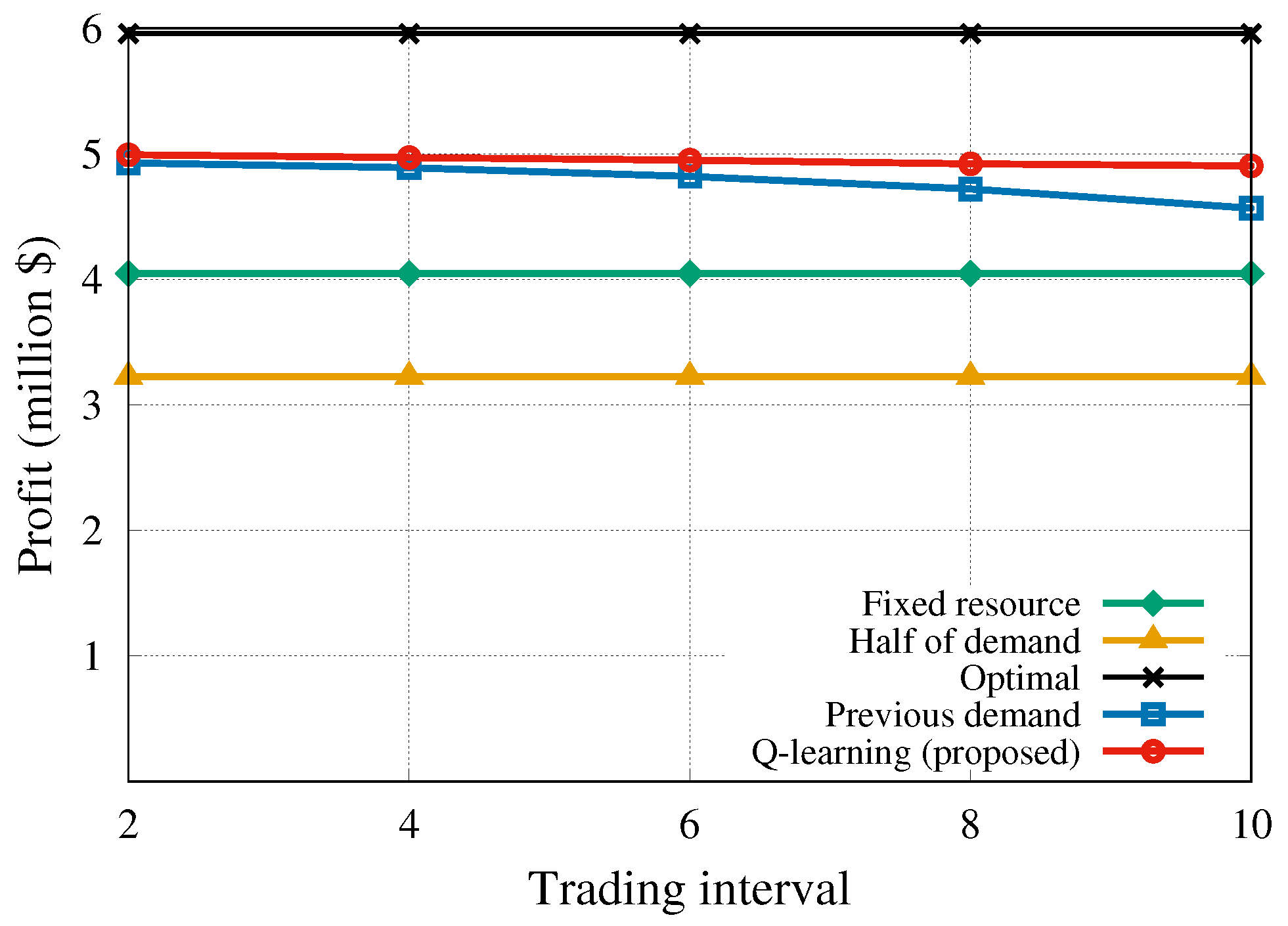
Figure 5 illustrates the comparison of the tenant profit achieved by the five algorithms. The static algorithms, i.e.,
half-of-demand and
fixed-resource, are not affected by the changes in the trading interval. The tenant has to pay for the resources that end-users do not actually use since the requested resources are statically provisioned. Therefore, there is no way to make an extra income from the unused resources resulting in a generally low profit. The dynamic strategies do not need to exclusively reserve resources every time, and they can trade the unused or additional resources at the next trading interval. As the trading interval increased, the
previous-slot-demand algorithm demonstrated a slightly decreasing profit because it did not consider future information, whereas the proposed algorithm was scarcely affected by the changes in the trading interval and earned the highest profit compared to the other algorithms.
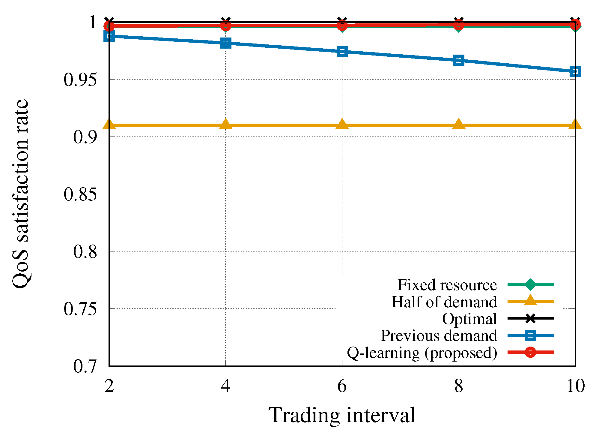
Figure 6 demonstrates that the proposed algorithm kept a very high QoS satisfaction rate because it allowed purchasing the required bandwidth in advance. This is the result of taking optimal actions according to the states for every
t on the basis of the state–action pairs, i.e., the Q-values. On the other hand, the QoS satisfaction rate achieved by
previous-slot-demand strategy decreased with the increasing trading interval. Similar to the previously stated result for this strategy, this indicates that the algorithm only focuses on the demand at the previous trading interval without considering the upcoming demand. The obtained results show that our algorithm works well even with a large trading interval to avoid the control overhead due to dynamic resource trading.
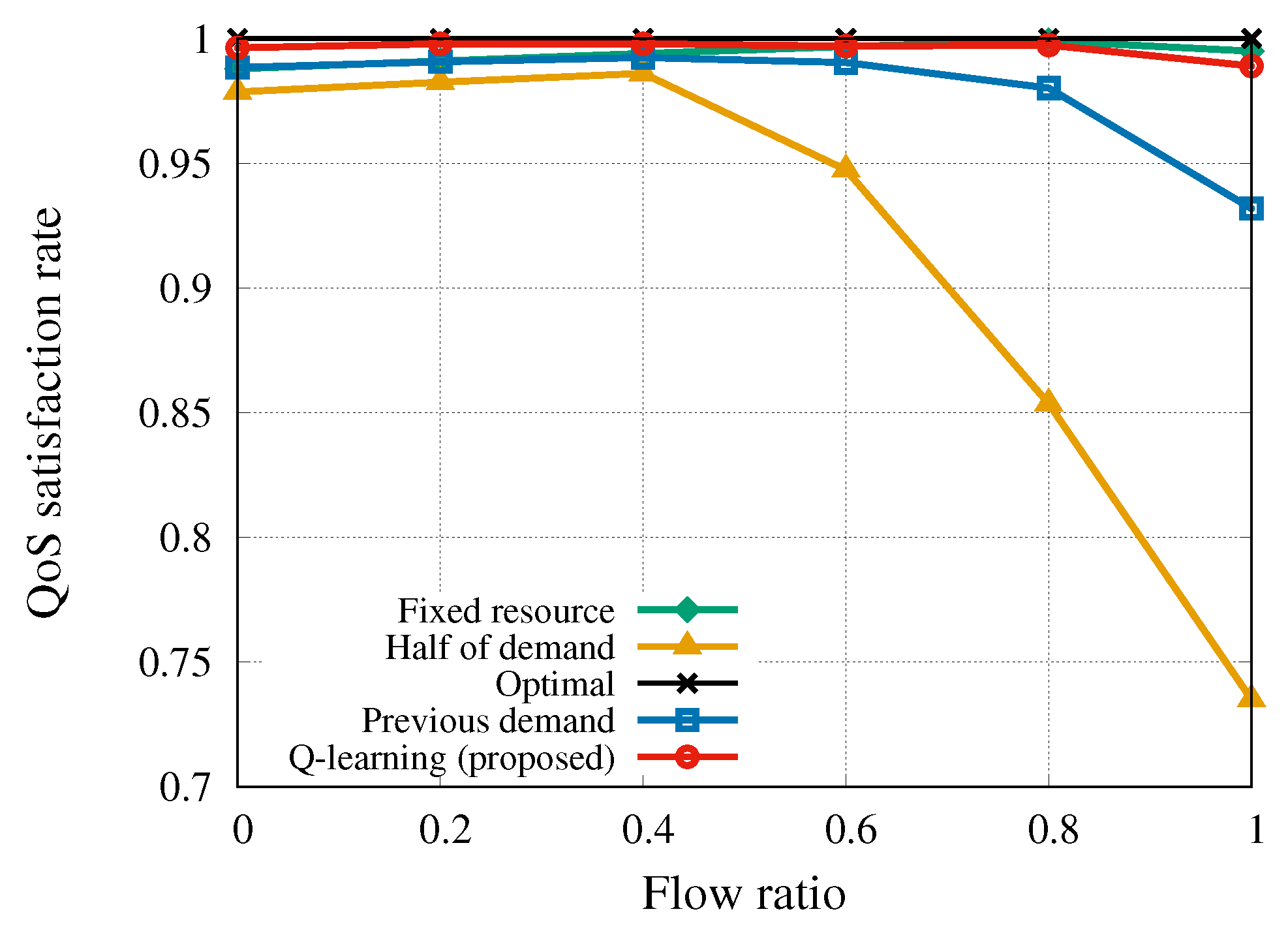
6.5. QoS Violation WITH Flow Ratio Change
To study the impact of the flow ratio on the algorithm performance, we plotted the QoS satisfaction rate of each algorithm according to the flow ratio
in Equation (
5). Note that we set the trading interval to 5 unless otherwise noted. Since inelastic flows usually require strict bandwidth, if the proportion of inelastic flows become large, the number of QoS violations may increase.
Indeed, the result illustrated in
Figure 7 demonstrates that the QoS satisfaction rate of all algorithms decreased as
increased in general. In particular, even though the
previous-slot-demand strategy is a dynamic adjustment algorithm, it depends upon the preceding information before trading interval
h. Since this algorithm did not prepare for sudden network traffic increase, QoS satisfaction rate decreased as the proportion of inelastic flows that require instantaneous bandwidth increased. Our algorithm guaranteed the QoS regardless of the inelastic flow ratio except in the case of the overwhelming number of inelastic traffic (of course pretty good performance). The result shows that our algorithm could adaptively determine how much amount of resource a tenant purchases in advance according to the inelastic flow ratio.
6.6. QoS Weight
We investigated the effect of penalty setting on the safety pursuit of the resource trading in Q-learning. In Equation (
11), the penalty is a function of the QoS weight
. The tenant putting a high value on the QoS satisfaction rate of end-users may set the QoS weight large for the Q-learning process. In this case, the tenant purchases more resources than it needs because it tends to pursue safety against QoS violations.
Figure 8 shows the total amount of the resource that the tenant trades during the lifetime of the slice. When a high QoS weight was applied, the tenant unnecessarily purchased more resources. This implies that a higher QoS weight can decrease the number of QoS violations but also lead to a lower profit.
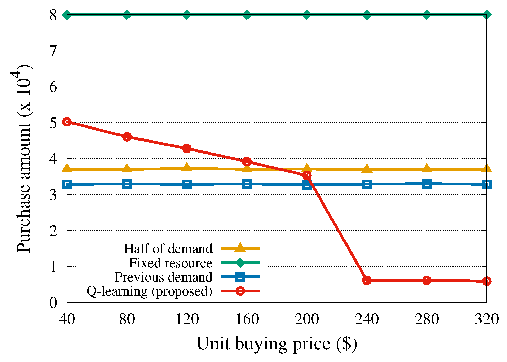
6.7. Adaptive Resource Trading Based on the Market Price
Finally, we investigated the effects of the pricing adjusted by the provider on the resource trading. We assumed that the buying price
is relative to the total allocated resource amount of all slices in Equation (
1). This is a consideration of the following two concerns in our business model. One concern is in terms of tenants: what should be done if sudden physical resource shortages arise due to increased traffic and increased resource requirements. It is reasonable to allow tenants to determine their resource amounts before a resource shortage occurs. The other concern is in terms of a provider, who pursues its profits as an independent business entity. As can be noticed in
Figure 9, only the proposed algorithm adjusted the purchase amount of the resource according to the buying price change. The change of the buying price may be caused by an increase in the total traffic volume of all slices. Since we set the selling price to
$200, purchasing resources at a buying price larger than
$200 would lead to a serious profit loss. Considering this fact, we can observe that our algorithm minimized the damage by reducing the amount of purchased resource when the unit buying price exceeded
$200. This result also indicates that the provider is able to manage and balance the allocation of limited resources through the price adjustments.


