Article

Incorporating Concentrating Solar Power into High Renewables Penetrated Power System: A Chance-Constrained Stochastic Unit Commitment Analysis

1
School of Electrical Engineering, Southeast University, Nanjing 210096, China
2
Jiangsu Provincial Key Laboratory of Smart Grid Technology and Equipment, Nanjing 210096, China
*
Author to whom correspondence should be addressed.
Appl. Sci. 2019, 9(11), 2340; https://doi.org/10.3390/app9112340
Submission received: 30 April 2019 / Revised: 30 May 2019 / Accepted: 1 June 2019 / Published: 6 June 2019
(This article belongs to the Special Issue Sustainable Energy Systems: Optimization and Efficiency)

Abstract

:
High renewables penetrated power systems would be greatly influenced by the uncertainty of variable renewable energy such as wind power and photovoltaic power. Unlike wind and photovoltaic plant, concentrating solar power with thermal energy storage has similar dispatchable characteristics as conventional thermal unit. Besides, thermal energy storage could support the coordinated operation of concentrating solar power with an electrical heater, which can be employed to convert surplus electricity in the grid into thermal power stored in thermal energy storage for further utilization. In this paper, concentrating solar power is incorporated into a chance-constrained two-stage stochastic unit commitment model. The model considers the energy and reserve services of concentrating solar power and the uncertainty of renewables. The proposed method is employed to assess the role of a concentrating solar power station with thermal energy storage and an electrical heater to provide grid flexibility in high renewables penetrated power systems. Numerical studies are performed on a modified IEEE 24-bus system to validate the viability of the proposed method for the day-ahead stochastic scheduling. The results demonstrate the economic and reliable value of concentrating solar power station to the improvement of unit commitment schedule, to the mitigation of wind uncertainty and photovoltaic uncertainty, and to the reduction of traditional unit reserve requirement. It is concluded that concentrating solar power with thermal energy storage and an electrical heater is effective in promoting the further penetration of renewables.

1. Introduction

The acceleration of renewable energy penetration is an irresistible trend of a power system to reduce energy crises and environmental problems [1]. However, compared with traditional thermal units, the variability and uncertainty of renewable energy such as wind power and solar photovoltaic (PV) pose great challenges to power system operation. Under the circumstance that the power system lacks operational flexibility, utilization of the costly electricity storage [2] and employment of the large amount of scheduled reserves [3] are common solutions to reduce the uncertainty of wind power and PV power. These methods lack cost-effectiveness in accommodating large-scale renewable energy.
In this light, the development of concentrating solar power (CSP) provides a new approach for renewable energy exploitability due to its dispatchability through using high-efficiency thermal energy storage (TES) [4]. Li et al. [5] and Gafurov et al. [6] simulated a sole TES system and a two-tank indirect TES system respectively and analyzed the dynamic characteristics of TES to provide flexible thermal energy. A CSP station with TES collects direct normal irradiation (DNI) during the daytime by converting it into thermal power, which is partially stored in TES and generates electricity as needed. Even in the cloudy day or at night, large-capacity TES enables CSP station to shift solar energy between different days to satisfy the load demand [7,8]. Besides, the capital cost of TES in a CSP station is $15/kWh, which is 1/10 of grid-connected electricity storage cost [9]. Furthermore, TES supports the coordinated operation between a CSP and electrical heater (EH). The incorporation of an EH enhances controllability of CSP to convert excess electricity in the power system into thermal energy for subsequent runs. In summary, the dispatchability of CSP with TES/EH would be an optimal choice to reduce renewable energy integration challenges and promote the power system to high renewables penetration.
Currently, much research is absorbed in the optimized operation strategy of CSP station [10,11] and economic benefit of a CSP station [12,13]. Additionally, the majority of works incorporated the CSP model into an electricity market, and addressed the strategic operation of CSP to maximize market profits [14,15]. With the increased CSP capacity, a CSP plant is definitely connected to the power system and receives the dispatching instructions. However, fewer studies analyzed the optimization of CSP operation from the perspective of the power system. Kroposki et al. [16] considered capitalized cost of the renewable energy and the transmission line, and discussed the probability of 100% renewables-dominated power system involving a CSP station. Jorge et al. [17] established a scheduling model to minimize the operating costs, and analyzed the economic benefits bought by the flexibility of a CSP in the renewable-dominated power system, however, the aspect of grid infrastructure expansion was not considered, where a CSP could provide cost advantages compared to other intermittent renewable technologies. Chen et al. [18] simulated a power system dispatching model with a CSP station to analyze the function of a CSP in reducing operating cost and renewables curtailment, however, the uncertainty of renewables was not considered. Du et al. [19] proposed a stochastic unit commitment (UC) and economic dispatch (ED) approach to evaluate the benefits of a CSP station for providing energy and extra reserve, but the results had geographical limitations and the simplified hypotheses needed further evaluation.
From the power system perspective, the optimization of a CSP station operation would not only concentrate on the energy services to reduce the overall operating cost of power system and increase renewables penetration, but also pays attention to the additional value of a CSP station to produce reserve services. Michael et al. [20] examined the mutual exclusion or complementarities among different benefits of a CSP station involving power generation profits, capacity benefits, reserve services and peak-shaving services. Pozo et al. [21] investigated the economic and advantages of a CSP reserve and EH reserve, but the results only verified the complementary effects among the CSP reserve and thermal unit reserve. In addition, there is a reasonable economic utilization range for renewable energy. The pursuit of 100% consumption would greatly increase the reserve scheduling cost and restrict the power system to receive more renewable energy, which greatly hinders the development of renewable energy. Luo et al. [22] set the minimum objective of the system power failure loss cost and the unit operating cost to optimize the system reserve, which could balance system economy and reliability. However, the global optimum results could not be guaranteed due to the spinning reserve and system operation were optimized separately. Wu et al. [23] formulated the chance constraints including loss-of-load probability (LOLP), reserve requirements and line flow limits, which were converted into a linear programming model and was solved by a decomposition-based method.
In this work, in order to estimate benefits of a CSP station in the high renewables penetrated power system, a chance-constrained stochastic unit commitment model with a CSP station is proposed. A scenario-based method is employed to represent the uncertainty of renewable energy [24,25]. The reserve planning method takes into account the chance constraints including “expected load not served (ELNS)” and “expected wind and solar curtailment (EWVS)” and optimizes reserve scheduling and system operation coordinately. The main contribution of our contributions can be summarized as follows.
(1)
A two stage stochastic UC model is established to research on the economic and reliable values of a CSP with TES/EH in the high renewables penetrated power system, concerning the uncertainty of wind power, PV and the solar energy received by CSP.
(2)
A chance-constrained method is employed in UC model to optimize the system reserves according to the scenario-based renewable energy forecast data.
(3)
The dispatchability and profitability of a CSP with TES/EH in unit commitment are verified through the comparative experiments among various system configurations.
The remainder of this paper is organized as follows. Section 2 describes the model of a CSP station with TES and EH equipment. Section 3 develops chance-constrained stochastic unit commitment model. A number of case studies based on IEEE-RTS 24 nodes system are carried out in Section 4 and discussed in Section 5. Finally, Section 6 concludes our research.

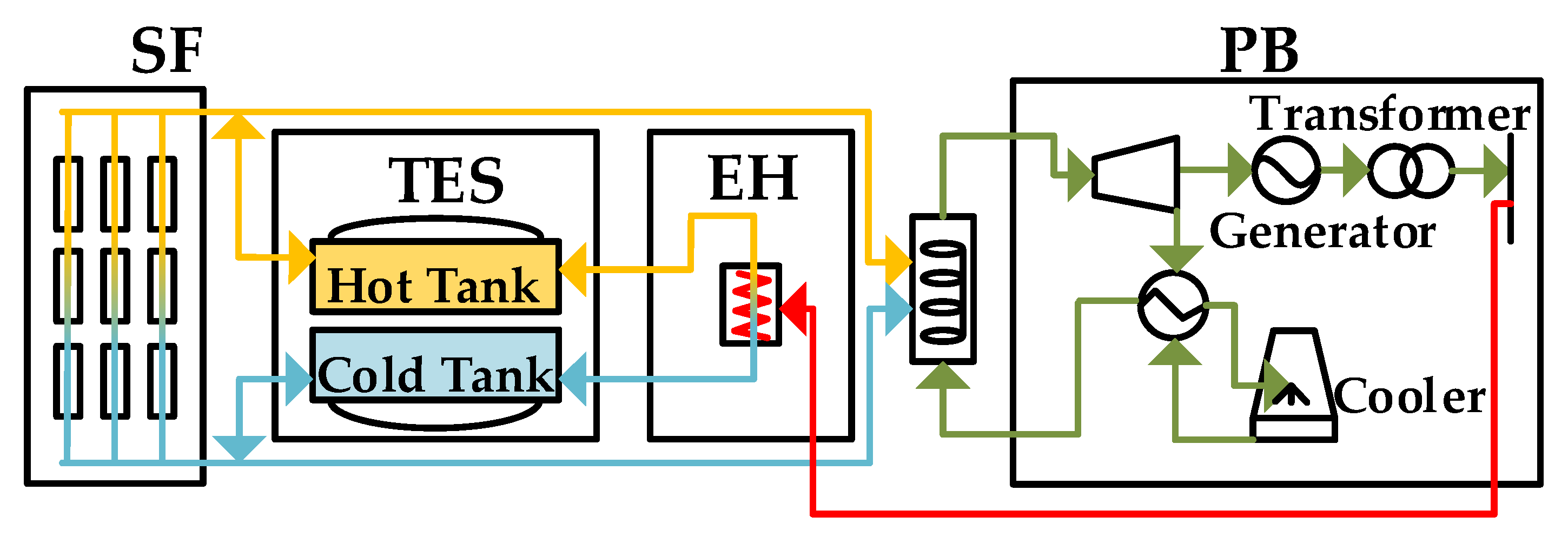
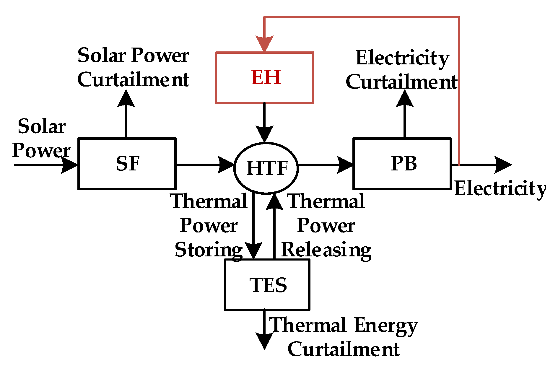
2. Model of Concentrating Solar Power (CSP) Station Equipped with Thermal Energy Storage (TES) and Electrical Heater (EH)

CSP utilizes solar power to generate electricity just like PV station, however, the conversion process of CSP is totally different from PV. CSP station is composed of four main parts, namely solar field (SF), TES system, power block (PB), additional EH equipment and the corresponding cleaning vehicle [26]. Heat transfer fluid (HTF) realizes the thermal cycling among different blocks. CSP station collects solar energy in SF to heat HTF. The heated HTF partially flows into PB to drive the steam turbine and then generates electricity. The rest of HTF could be stored in TES as thermal energy to be further used [27]. The capability of CSP station to utilize TES system makes CSP a dispatchable resource as thermal unit. EH equipment could absorb excess electricity in the power system and convert it into thermal energy to be stored in the TES system for later conversion. Therefore, EH could exploit the excess room of TES and expand the operating range of CSP station. The detailed configuration of grid-connected CSP station is illustrated in Figure 1.
From the aspect of the power dispatching system, the model of CSP station could ignore the short-time dynamic process of energy exchange, and concentrate on the power flow and operation constraints among different modules [28]. Based on the operation mechanism of CSP, this paper proposes a linear steady-state dispatch model of a CSP station which is applicable for the incorporation into the dispatching system. The operating state of a grid-connected CSP station with TES and EH equipment could be reflected by mixed integer linear constraints. The simplified energy flow is illustrated in Figure 2.
From the perspective of HTF, the energy flowing into a CSP station involves two main parts: thermal energy from SF ( q c , t S F _ H T F ) and thermal energy from EH ( q c , t E H _ H T F ). Correspondingly, the energy consumed by a CSP station includes thermal energy exchange of TES ( q c , t H T F _ T E S q c , t T E S _ H T F ) and thermal energy consumption by PB ( q c , t H T F _ P B ). The possible thermal energy dissipation is the solar power curtailment in SF and the loss in charging and discharging process, which is embodied in the efficiency parameters. The power balance can be expressed by Equations (1)–(4).
q c , t S F _ H T F + q c , t E H _ H T F =   ( q c , t H T F _ T E S q c , t T E S _ H T F ) + q c , t H T F _ P B   , t , c
q c , t S F _ H T F = q c , t S F , 0 p c , t C S P , c u r / η c P B   , t , c
q c , t T E S , c h a = η c T E S , c h a q c , t H T F _ T E S   , t , c
q c , t T E S , d i s = q c , t T E S _ H T F / η c T E S , d i s   , t , c
where, q , c , t S F is the point forecast of thermal power converted from solar power; P c , t C S P , c u r represents the possible power spillage of CSP station; η c P B means the efficiency of PB; q c , t T E S , c h a , q c , t T E S , d i s stand for the actual charging and discharging thermal power of the TES system respectively; η c T E S , c h a , η c T E S , d i s represent the charging and discharging efficiency of the TES system respectively.
The TES system possesses three operating states: charging, discharging and thermal equilibrium. The thermal power balance and the upper-lower limits are given by Equations (5) and (6). Besides, during the operation day, the state of charge (SOC) of the TES system is assumed to restore to the initial state at the end of the day which is shown in Equation (7).
E c , t T E S = ( 1 γ c T E S ) E c , t 1 T E S + ( q c , t T E S , c h a q c , t T E S , d i s ) Δ t   , t > 1   , c
E c T E S , + E c , t T E S E c T E S ,   , t , c
E c , t T E S = E c , t + 23 T E S   , t = 1 ,   c
where, E c , t T E S , E c , t 1 T E S represent the SOC of TES at time t and t − 1; Thermal energy loss is represented by parameter γ c T E S ; △t stands for the time interval; E + c T E S , , E c T E S , show the upper-lower limits of the SOC of TES.
Equations (8) and (9) set the charging and discharging rate of the TES system. When the on/off state variables of charging function ( o c , t T E S , c h a ) and discharging function ( o c , t T E S , d i s ) are equal to 1, the feasible interval of charging and discharging rate of TES system is [0, q c T E S , m a x ].
0 q c , t T E S , d i s o c , t T E S , d i s q c T E S , m a x   , t , c
0 q c , t T E S , c h a o c , t T E S , c h a q c T E S , m a x   , t , c
Equations (10)–(12) describe the relationship between the on/off state variable and the starting-up variable. The charging and discharging state could not happen simultaneously, and the TES discharging would arise only if the PB on/off state variable ( o c , t P B ) is equal to 1. If the TES charging state is on, EH could absorb energy from the grid and the EH on/off state variable ( o c , t E H ) is equal to 1.
o c , t T E S , c h a + o c , t T E S , d i s 1   , t , c
o c , t T E S , d i s o c , t P B   , t , c
o c , t T E S , c h a o c , t E H   , t , c
Concerning the PB system, this paper shows the linear relationship between the input thermal energy ( q c , t H T F _ P B ) and the output power of PB ( p c , t C S P ) shown in Equation (13). Equation (14) guarantees the power output range of PB system [ P c P B , m i n , P c P B , m a x ] when the PB system is on ( o c , t P B = 1).
η c P B ( q c , t H T F _ P B u c , t P B E c P B , s t ) = P c , t C S P   , t , c
o c , t P B P c P B , min P c , t C S P o c , t P B P c P B , max   , t , c
where, u c , t P B denotes the start-up variable of PB; E c P B , s t represents the initial power needed to start the PB system.
The power output of the EH ( p c , t E H ) is constrained between [ P c E H , m i n , P c E H , m a x ] when the on/off variable of EH is on ( o c , t E H = 1) which is shown in Equation (15).
o c , t E H P c E H , min P c , t E H o c , t E H P c E H , max   , t , c
The power output of the grid-connected CSP station ( P c , t N E T ) is denoted by Equation (16).
P c , t N E T = P c , t C S P P c , t E H   , t , c
The power output of PB has the similar constraints to the thermal units, such as the ramping constraints shown in Equations (17) and (18) and the minimum on/off time constraints described in Equations (19) and (20).
P c , t C S P P c , t 1 C S P ( 2 o c , t 1 P B o c , t P B ) P c P B , m i n + ( 1 + o c , t 1 P B o c , t P B ) Δ P c P B , u p   , t > 1 , c
P c , t 1 C S P P c , t C S P ( 2 o c , t 1 P B o c , t P B ) P c P B , m i n + ( 1 o c , t 1 P B + o c , t P B ) Δ P c P B , d n   , t > 1 , c
where, P c P B , u p , P c P B , d n formulate the upper-lower limit of ramping rate respectively.
( o c , t P B o c , t 1 P B ) T c , min P B , o n + τ = t T c , min P B , o n 1 t 1 o c , τ P B 0   , t > 1 , c
( o c , t 1 P B o c , t P B ) T c , min P B , o f f + τ = t T c , min P B , o f f 1 t 1 ( 1 o c , τ P B ) 0   , t > 1 , c
where, T c , m i n P B , o n , T c , m i n P B , o f f represent the minimum on time and off time respectively.
Other related constraints of CSP station are depicted in Equations (21)–(23).
o c , t P B o c , t 1 P B u c , t P B   , t > 1 , c
u c , t P B o c , t P B   , t , c
u c , t P B 1 o c , t 1 P B   , t > 1 , c

3. Chance-Constraint Two-Stage Stochastic Unit Commitment

3.1. Uncertainty of Renewables

In this section, renewable energy scenarios are generated for the stochastic UC program. In this paper, s represents the index of second-stage scenario from 1 to Ns. The time interval t is set a 1 h. Wind generation fluctuation ( w w , t , s W I N D , f o r e ), PV generation fluctuation ( v v , t , s P V , f o r e ) and solar power fluctuation in SF of CSP station ( q c , t , s S F , f o r e ) are considered as random functions. In this paper, the point forecast of load is generally hypothesized to be accurate, in other words, the uncertainty of load is ignored. The point forecast of load is L n , t 0 .
Probabilistic forecasting is the widely used method to provide the inherent uncertainty of renewables [29]. For a given point forecast of renewable energy, probability distribution functions are necessary to gain the future realization of renewables [30]. Currently, much previous research concerns the probability distribution functions, involving Gaussian distribution function [31], Beta distribution function [32,33] and truncated normal distribution function [34]. In this paper, network constraints are not involved in the proposed model. Therefore, because of the central limit theorem, the wind and PV production random functions could be simply described by Gaussian distributions with zero-mean Gaussian distributed errors within each time interval [21,35].
The wind power distribution function is described as Equation (24).
w w , t , s W I N D , f o r e N ( w w , t W I N D , 0 , σ w , t W I N D , v ) = w w , t W I N D , 0 + e w , t , s W I N D , e ,   t , w , s
where, w w , t W I N D , 0 represents the point forecast of wind power; e w , t , s W I N D , e denotes the zero-mean Gaussian distributed forecast errors.
The PV distribution function is described as Equation (25).
v v , t , s P V , f o r e N ( v v , t P V , 0 , σ v , t P V , v ) = v v , t P V , 0 + e v , t , s P V , e ,   t , v , s
where, v , v , t P V represents the point forecast of PV station; e v , t , s P V , e denotes the zero-mean Gaussian distributed forecast errors.
As for the CSP station, it is acknowledged that CSP is a partially dispatchable resource, however, in order to guarantee the credibility and stability of the results, the uncertainty of solar power in the SF section could not be simply ignored. More specifically, although the power output of the CSP station has no direct relationship with the instantaneous irritation owing to the large-capacity TES system, problems would come because the SOC of the TES system should restore to the initial state at the end of the day [3]. The storage level of TES would be affected by the uncertain DNI absorbed from the SF capsule, and would influence the power output of CSP. Therefore, it is necessary to take into account the uncertainty of solar energy received by SF in the stochastic scenarios. The CSP distribution function is described as Equation (26).
q c , t , s S F , f o r e N ( q c , t S F , 0 , σ c , t S F , v ) = q c , t S F , 0 + e c , t , s S F , e ,   t , c , s
where, q c , t S F , 0 is the point forecast of thermal energy converted from solar power; e c , t , s S F , e denotes the zero-mean Gaussian distributed forecast errors.
The net equivalent load is defined as the difference between load and the power output of wind power and PV power described in Equation (27). Equation (28) describes the mean and variance of the net equivalent load. CSP is assumed to be the controllable resource as a thermal unit.
L t , s E Q , f o r e = n = 1 N N L n , t 0 ( w = 1 N W w w , t , s W I N D , f o r e + v = 1 N V v v , t , s P V , f o r e ) ,   t , s N ( L t E Q , 0 , σ t )
L t E Q , 0 = n = 1 N N L n , t 0 ( w = 1 N W w w , t W I N D , 0 + v = 1 N V v v , t P V , 0 ) ,   t σ t 2 = ( N W σ w , t W I N D , v ) 2 + ( N V σ v , t P V , v ) 2 ,   t
Finally, based on the Gaussian distribution in each hour, a Latin hypercube sampling (LSH) technique [29] is employed to generate an appropriate number of power scenarios. Compared with Monte Carlo sampling, LSH adopts the stratified sampling method which could restore the probability distribution function with fewer samples [36]. The K-means clustering algorithm [37] is employed for the scenario reduction with little loss of statistical information. The reduced scenario sets could approximately represent the original power scenarios and could be calculated in unit commitment easily. Each scenario is associated with a scenario probability.

3.2. Scenario-Based Day-Ahead Unit Commitment

Oriented to the high renewables penetrated system, the proposed model of two-stage chance-constraint stochastic unit commitment could be used to optimize the day-ahead power generation scheme. With the consideration of the intermittency of renewable energy, power generation scheduling and spinning reserve scheduling are optimized simultaneously in the stochastic UC model. Furthermore, based on chance-constrained optimization, a reserve planning method is proposed to balance system reliability and economy, concerning thermal unit reserves and CSP reserves.
Day-ahead UC programming is separated into two parts. Based on the point forecast of renewables, the first stage of UC model optimizes the expected day-ahead generation, start-up and reserve decisions of each plant. The second stage of UC model is formulated to guarantee that the decisions made in the first stage could be deployed to handle the deviation between the expected point forecast of renewables and the probabilistic forecast of renewables in each pre-decided scenario.
In this paper, the proposed reserve decision planning is different from the traditional planning model. The traditional reserve decision making usually adopts spinning reserve according to the historical experience, and lacks reliability and economy [38,39]. In order to address the above issue, the chance-constraint reserve planning model is proposed to ensure that under various stochastic scenarios, the scheduled reserves could satisfy the system reliability requirements (EENS, EWVS) within the specified probability. Meanwhile, the reliability requirements are introduced in the objective function concerning economic dispatch. Therefore, the proposed reserve planning guarantees the reliable and economic requirements simultaneously.

3.2.1. Objective

The objective of UC model is to reduce the system operating costs (CostSys) including generation scheduling costs and economic dispatch costs. Generation scheduling costs (CostGC) are the first stage day-ahead costs, involving the fuel cost, the start-up cost and the reserve scheduling cost for the thermal units. Economic dispatch costs (CostDC) are the second stage costs, including the scenario-based spinning reserve deploying cost for thermal unit, the generating cost for the CSP and EH, and the penalty cost for load shedding and renewables spillage. The detailed objective is depicted in Equation (29).
m i n   Cos t S y s = Cos t G C + Cos t D C = t = 1 N T { g = 1 N G ( C g , t G + S T g , t G + C g G , u p R g , t G , u p + C g G , d n R g , t G , d n ) + s = 1 N S π s [ g = 1 N G ( c g G , u p r g , t , s G , u p + c g G , d n r g , t , s G , d n ) + c = 1 N C ( C c C S P P c , t , s C S P + C c E H P c , t , s E H ) + n = 1 N N c L L n , t , s c u r +   w = 1 N W c W P w , t , s W , c u r + v = 1 N V c V P v , t , s P V , c u r + c = 1 N C c P P c , t , s C S P , c u r ] }
where, C g , t G , S T g , t G represent the fuel cost and the start-up cost for thermal unit respectively; C g G , u p , C g G , d n stand for the coefficient of up/down reserve scheduling cost for thermal unit respectively; R g , t G , u p , R g , t G , d n describe the scheduled up/down reserve for thermal unit respectively; c g G , u p , c g G , d n are the coefficient of up/down reserve deploying cost for thermal unit respectively; r g , t , s G , u p , r g , t , s G , d n denote the deployed up/down reserve for thermal unit in stochastic scenarios respectively; C c C S P , C c E H are defined as the coefficient of CSP and EH generating costs, respectively; P c , t , s C S P , P c , t , s E H formulate the power output of the CSP and EH in stochastic scenarios respectively; cL, cW, cV, cP represent the coefficient of penalty costs for load shedding, wind power spillage, PV spillage and CSP spillage respectively; L n , t , s c u r , P w , t , s W , c u r , P v , t , s P V , c u r , P c , t , s C S P , c u r respectively demonstrate the quantity of load shedding, wind power spillage, PV spillage and CSP spillage; πs is the scenario probability. NT shows the time span of the test. NS, NG, NN, NW, NV and NC illustrate the quantity of scenarios, thermal units, load, wind stations, PV stations and CSP stations.

3.2.2. The First-Stage Constraint

The first stage is employed to optimize the day-ahead generation, start-up and scheduled reserve decisions for each plant. The first stage constraints are based on the point forecast of wind and solar power.
(1) Thermal unit constraints
Equations (30) and (31) set the minimum on and off time constraints. The relationships between unit status variables and start-up variables are described by Equation (32). Equations (33) and (34) show the ramping limits. Equations (35)–(37) ensure the capability of thermal units to provide reserve services within the operating range.
( o g , t G o g , t 1 G ) T g , min G , o n + τ = t T g , min G , o n 1 t 1 o g , τ G 0   , t > 1 , g
( o g , t 1 G o g , t G ) T g , min G , o f f + τ = t T g , min G , o f f 1 t 1 ( 1 o g , τ G ) 0   , t > 1 , g
o g , t G o g , t 1 G u g , t G , u g , t G o g , t G , u g , t G 1 o g , t 1 G   , t > 1 , g
P g , t G P g , t 1 G ( 2 o g , t 1 G o g , t G ) P g G , m i n + ( 1 + o g , t 1 G o g , t G ) Δ P g G , u p   , t > 1 , g
P g , t 1 G P g , t G ( 2 o g , t 1 G o g , t G ) P g G , m i n + ( 1 o g , t 1 G + o g , t G ) Δ P g G , d n   , t > 1 , g
P g , t G + R g , t G , u p o g , t G P g G , m a x   , t , g
P g , t G R g , t G , d n o g , t G P g G , m i n   , t , g
0 R g , t G , u p o g , t G R g G , u p , + ,   0 R g , t G , d n o g , t G R g G , d n , +   , t , g
where, o g , t G , o g , t 1 G are the status variable of thermal unit at time t and t − 1 respectively; u g , t G represents the start-up variables of thermal unit; T g , m i n G , o n , T g , m i n G . o f f respectively denote the minimum on and off time; P g , t G , P g , t 1 G represent the power output of thermal unit at time t and t − 1 respectively; P g G , m a x , P g G , m i n stand for the maximum and minimum power output of thermal unit respectively; P g G , u p , P g G , d n describe the up and down ramping limit for thermal unit respectively; R g , t G , u p , R g , t G , d n describe the scheduled up/down reserve for thermal unit respectively. R , + g G , u p , R + g G , d n , denote the maximum up and down reserve for thermal unit to ensure the generation efficiency respectively.
The start-up cost includes the hot start cost and the cold start cost. For each thermal unit, the start-up cost ( S T g , t G ) is classified by the idle time of unit before it is starts, namely start-up time. The set maximum hot start-up time m, and the test time M determine the classification of the start process. Where, Kg,n is the coefficient of the start-up cost; hcg represents the coefficient of the hot start cost; ccg decides the coefficient of the cold start cost. The piecewise linearized Equation (38) is formulated in which the start-up time between 0 and m − 1 would be classified as hot start, and the time between m and M would be considered as a cold start.
{ S T g , t G K g , n ( o g , t G n = 1 M o g , t n G ) S T g , t G 0 K g , 1 : m 1 = h c g , K g , m : M = c c g   , t , g
The piecewise linearized Equation (39) calculates the fuel cost of thermal unit.
C g , t G a g , t P g , t G + b g , t o g , t G   , t , g
where, ag,t and bg,t represent the coefficient of fuel cost.
(2) CSP and EH constraints
The operation constraints of the CSP and EH are described in the feasible operation space shown in Equations (1)–(23).
When incorporated into the power system, CSP and EH provide energy services as well as reserve services.
Equations (40)–(44) demonstrate the up/down spinning reserve scheduling constraints of TES system. When the PB system is on, the up spinning reserve ( R c , t P B , u p ) is limited by the upper limit of PB operating range and the room of available power releasing of TES system. Similarly, the down spinning reserve ( R c , t P B , d n ) is constrained by the lower limit of operation space and the remaining space of the TES system.
R c , t P B , u p o c , t P B ( P c P B , m a x P c , t C S P )   , t , c
R c , t P B , u p o c , t P B (   E c , t T E S E c T E S , ) η c P B   , t , c
R c , t P B , d n o c , t P B ( P c , t C S P P c P B , m i n )   , t , c
R c , t P B , d n o c , t P B (   E c T E S , +   E c , t T E S ) η c P B   , t , c
0 R c , t P B , u p o c , t P B R c P B , u p , + , 0 R c , t P B , d n o c , t P B R c P B , d n , +   , t , c
where, R c P B , u p , + , R c P B , d n , + denote the maximum up and down reserve for each unit to ensure the generation efficiency.
Equations (40)–(43) are composed of bilinear terms which belong to the non-deterministic polynomial hard (NP-Hard) problem. This kind of problem could not be calculated directly only if it is linearized. In this paper, the McCormick convex envelope method, namely Big-M method, is utilized to linearize the bilinear terms [39]. The detailed method is shown in Appendix A.
Equations (45)–(47) demonstrate the up/down spinning reserve scheduling constraints of EH equipment. By contrast with the CSP plant and the traditional thermal unit, the EH equipment consumes the excess electricity in the power system and responds quickly without set ramping rate. The EH provides up spinning reserve ( R c , t E H , u p ) and down spinning reserve ( R c , t E H , d n ) through decreasing and increasing electricity consumptions.
P c , t E H R c , t E H , u p o c , t E H P c E H , min   , t , c
P c , t E H   +   R c , t E H , d n o c , t E H P c E H , m a x   , t , c
0 R c , t E H , u p o c , t E H R c E H , u p , + , 0 R c , t E H , d n o c , t E H R c E H , d n , +   , t , c
where, o c , t E H is the status variable of EH; R c E H , u p , + , R c E H , d n , + denote the maximum up and down reserve for each EH unit.
(3) Wind power and photovoltaic (PV) constraints
Equations (48) and (49) formulate the power output range of wind power and PV station. The wind power ( P w , t W I N D ) and the PV power ( P v , t P V ) are definitely lower than the point forecast of wind power and PV power ( w w , t W I N D , 0 , v v , t P V , 0 ) and allow for the renewables spillage.
0 P w , t W I N D w w , t W I N D , 0   , t , w
0 P v , t P V v v , t P V , 0   , t , v
(4) System constraints
The system power balance is formulated in Equation (50) to guarantee the power output to meet the load requirement at each time. In the first stage, load shedding is not permitted.
w = 1 N W P w , t W I I N D + v = 1 N V P v , t P V + g = 1 N G P g , t G + c = 1 N C ( P c , t C S P P c , t E H ) = n = 1 N N L n , t 0   , t
Equations (51) and (52) set the scheduled up reserve range is [ R t u p , , R t u p , + ], and the scheduled down reserve range is [ R t d n , , R t d n , + ].
R t u p , g = 1 N G R g , t G , u p + c = 1 N C ( R c , t P B , u p + R c , t E H , u p ) R t u p , +   , t
R t d n , g = 1 N G R g , t G , d n + c = 1 N C ( R c , t P B , d n + R c , t E H , d n ) R t d n , +   , t
(5) Chance-constraints
The reliability requirements at time t is described in the chance-constrained manner and are shown in Equations (53) and (54). Under the circumstances that the CSP reserve and the thermal unit reserve are considered, the load shedding case Equation (53) at time t is bounded by b t l with the probability greater than α t l . A similar formulation in Equation (54) could be used for the renewables spillage limit. The chance-constraints must be converted into the equivalent deterministic formulations to be employed in the UC model. The detailed introduction of chance-constrained reserve planning as well as the linearized conversion method is described in Section 3.3.
Pr { E L N S t b t l ] } a t l   , t
Pr { E W V S t b t w v ] } a t w v   , t

3.2.3. The Second-Stage Constraint

The first stage utilizes the point forecasts to estimate the UC decisions and the scheduled reserve decisions. In the second stage, the uncertainty of renewables is considered and Ns pre-determined scenarios are generated using the method proposed in Section 3.1. In each pre-decided scenario, the second stage constraints guarantee the first stage decisions to be appropriately deployed to satisfy the power deviations of renewable energy.
(1) Thermal unit constraints
Equation (55) formulates the dispatched power output of each unit which equals to the day-ahead power output in the first stage plus the reserve deployment in the second stage.
P g , t , s G = P g , t G + r g , t , s G , u p r g , t , s G , d n ,   t , g , s
Equations (56)–(58) demonstrate that the deployed reserve is constrained within the capacity of the scheduled reserve and the up/down reserve deployment would not happen simultaneously. Equations (59)–(61) describe the other thermal unit constraints.
0 r g , t , s G , u p o g , t , s G , u p _ d e p l o y R g , t G , u p ,   t , g , s
0 r g , t , s G , d n o g , t , s G , d n _ d e p l o y R g , t G , d n ,   t , g , s
o g , t , s G , u p _ d e p l o y + o g , t , s G , d n _ d e p l o y 1 ,   t , g , s
o g , t , s G = o g , t G ,   t , g , s
o g , t , s G P g G , m i n P g , t , s G o g , t , s G P g G , m a x ,   t , g , s
( Other   constraints   are   the   modified   function   of   30 31 , 33 34 )
where, Equations (56) and (57) should be linearized by the Big-M method; P g , t , s G stands for the power output in the second stage; r g , t , s G , u p , r g , t , s G , d n represent the up/down deployed reserve in stochastic scenario; o g , t , s G , u p _ d e p l o y , o g , t , s G , d n _ d e p l o y stand for the on/off variable of the up reserve deployment and the down reserve deployment respectively. o g , t , s G represents the on/off state variable of thermal unit in the second stage. In Equation (61), the modified function has the stochastic properties, while the subscript s (the index of second-stage scenario from 1 to NS) should be added to these modified equations. This idea also applies for the following equations.
(2) CSP and EH constraints
Equations (62)–(65) demonstrate the power output range of the CSP station in the second stage. Equations (66)–(69) depict the power output range of the EH equipment. Equations (70)–(73) formulate the other CSP and EH constraints.
P c , t , s C S P = P c , t C S P + r c , t , s P B , u p r c , t , s P B , d n ,   t , c , s
0 r c , t , s P B , u p o c , t , s P B , u p _ d e p l o y R c , t P B , u p ,   t , c , s
0 r c , t , s P B , d n o c , t , s P B , d n _ d e p l o y R c , t P B , d n ,   t , c , s
o c , t , s P B , u p _ d e p l o y + o c , t , s P B , d n _ d e p l o y 1 ,   t , c , s
P c , t , s E H = P c , t E H r c , t , s E H , u p + r c , t , s E H , d n ,   t , c , s
0 r c , t , s E H , u p o c , t , s E H , u p _ d e p l o y R c , t E H , u p ,   t , c , s
0 r c , t , s E H , d n o c , t , s E H , d n _ d e p l o y R c , t E H , d n ,   t , c , s
o c , t , s E H , u p _ d e p l o y + o c , t , s E H , d n _ d e p l o y 1 ,   t , c , s
o c , t , s P B = o c , t P B ,   t , c , s
o c , t , s P B P c P B , m i n P c , t , s C S P o c , t , s P B P c P B , m a x ,   t , c , s
o c , t , s E H P c E H , m i n P c , t , s E H o c , t , s E H P c E H , m a x ,   t , c , s
( Other   constraints   are   the   modified   function   of   1 20 )
where, Equations (63), (64), (67) and (68) should be linearized by Big-M method; P c , t , s C S P , P c , t , s E H stand for the power output of the CSP and EH respectively in the second stage; r c , t , s P B , u p , r c , t , s P B , d n represent the up/down deployed reserve for CSP in the stochastic scenario; r c , t , s E H , u p , r c , t , s E H , d n represent the up/down deployed reserve for EH in the stochastic scenario; o c , t , s P B , u p _ d e p l o y , o c , t , s P B , d n _ d e p l o y , o c , t , s E H , u p _ d e p l o y , o c , t , s E H , d n _ d e p l o y stand for the on/off variable of the up reserve deployment and down reserve deployment for the CSP and EH system respectively. o c , t , s P B , o c , t , s E H stand for the on/off state variable of the CSP in the second stage.
(3) Wind power and PV constraints
The second stage power output of wind power and PV station are guaranteed in Equation (74).
( Modified   function   of   48 49 )
(4) System constraints
The second stage power balance is demonstrated in Equations (75) and (76). Load shedding is permitted in the second stage.
w = 1 N W P w , t , s W I I N D + v = 1 N V P v , t , s P V + g = 1 N G P g , t , s G + c = 1 N C ( P c , t , s C S P P c , t , s E H ) = n = 1 N N ( L n , t 0 L n , t , s c u r ) , t , s
0 L n , t , s c u r L n , t 0 ,   t , n , s
P w , t W I N D , P v , t , s P V stand for the power output of wind and PV respectively in the second stage. L n , t , s c u r represents the loss of load in the stochastic scenario.

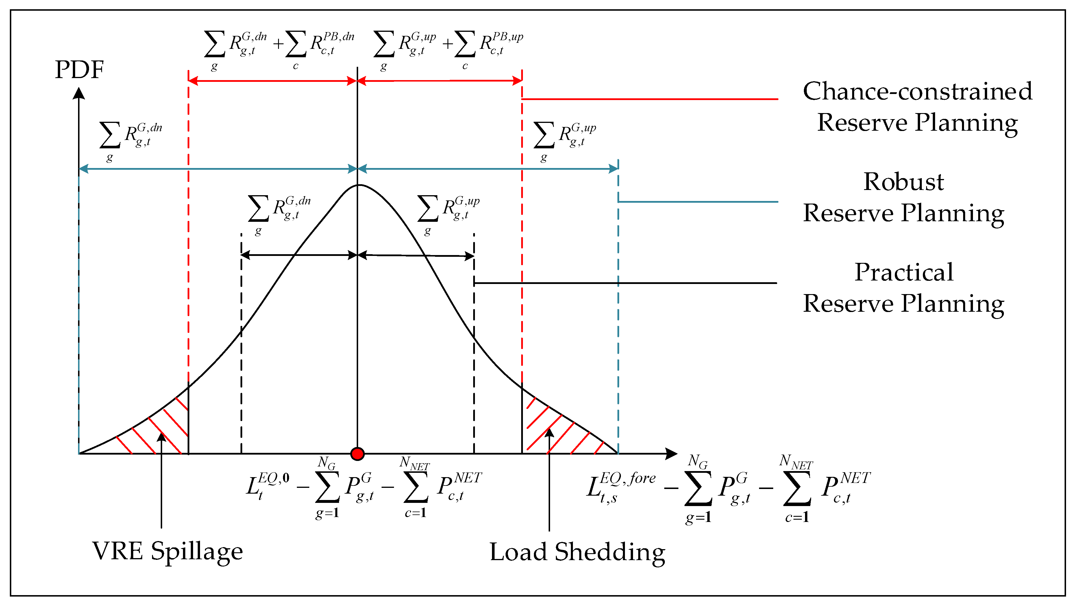
3.3. Chance-Constrainted Reserve Planning Model

In the traditional reserve planning model, the scheduled reserve is usually set as a constant value at each time and thermal unit provides the only reserve service in the power system. Specially, in the robust reserve planning, a significant number of reserves are scheduled to satisfy any kind of renewable energy deviations. Nevertheless, some extreme renewable energy outputs have low possibilities and there is no need to meet these demands [40]. Besides, in the practical reserve planning model, the capacity of the scheduled reserve is set as a certain percentage of system load and the additional reserve is considered in accordance with the renewables uncertainty. However, this method is not applicable for the power system with high renewables penetration, which has increased power output uncertainty [41].
Therefore, to handle the problems above, a chance-constrained reserve planning model is proposed in this paper which is introduced as follows. Figure 3 illustrates the chance-constrained reserve scheduling strategy.
From Equation (27), we know that the equivalent load obeys the Gaussian distribution in each hour, which is clearly shown in Equation (77).
L t , s E Q , f o r e = n = 1 N N L n . t 0 w = 1 N W w w , t , s W I N D , f o r e v = 1 N V v v , t , s P V , f o r e N ( n = 1 N N L n , t 0 w = 1 N W w w , t W I N D , 0 v = 1 N V v v , t P V , 0   ,   ( N W σ w , t W I N D , v ) 2 + ( N V σ v , t P V , v ) 2 ) N ( L t E Q , 0   ,   σ t 2 )
(1) Load shedding
When the power output of renewable energy in the stochastic scenario is lower than the expected point forecast, there is a chance that the power from thermal units, renewable energy could not satisfy the power balance considering the overall system up reserves (thermal unit reserves and CSP reserves).
The expected value of loss-of-load probability (LOLP) is defined as “expected load not served” (ELNS) which is shown in Equation (78). E represents the expected value.
E L N S t =   E [ F t ( s ) | F t ( s ) 0 ]
where, Ft(s) is shown in Equation (79).
F t ( s ) = L t , s E Q , f o r e g = 1 N G ( P g , t G + R g , t G , u p ) c = 1 N C ( P c , t C S P + R c , t P B , u p P c , t E H )
The probabilistic constraints concerning ELNS is depicts in Equation (80). Pr represents the probability value.
Pr { E L N S t b t l ] } a l
(2) Renewables spillage
When the stochastic renewable energy power appears higher than the expected point forecast, a chance occurs when the power from generators exceed the load demand after the utilization of the total system down reserves.
The expected value of wind power and PV spillage probability is defined as “expected wind and PV spillage” (EWVS) which is shown in Equation (81).
E W V S t = E [ H t ( s ) | H t ( s ) 0 ]
where, Ht(s) is shown in Equation (82).
H t ( s ) = L t , s E Q , f o r e g = 1 N G ( P g , t G R g , t G , d n ) c = 1 N C ( P c , t C S P R c , t P B , d n P c , t E H )
The probabilistic constraints concerning EWVS is depicts in Equation (83).
Pr { E W V S t b t w v ] } a w v
Equations (80) and (83) should be converted into the equivalent deterministic formulations to be employed in the UC model [35].
Given the parameter αl, αwv, b t l , b t w v , the equivalent deterministic formulations could be described in Equations (84)–(86).
E L N S t = 1 1 α l s = 1 N s p ( s ) z t ( s ) b t l
E W V S t = 1 1 α w v s = 1 N s p ( s ) y t ( s ) b t w v
0 z t ( s ) F t ( s ) , 0 y t ( s ) H t ( s )  
where, p(s) represents the probability of scenario S; zt(s) is the maximum value of 0 and Ft(s); yt(s) is the maximum value of 0 and −Ht(s).

4. Results

In this section, cases are carried out based on the IEEE reliability test system. Case studies are disposed of YALMIP (a MATLAB toolbox) [42] and are solved using CPLEX12.8.0 (an optimization software) on a PC with a 2.20 GHz Intel processor and 8.0 RAM.

4.1. Test System

All the case studies have been tested on the modified 24-bus IEEE reliability test system, involving 24 nodes, 15 generators. The detailed parameters could be referred to in [43]. In this paper, the time period is 24 h with the time interval 1 h. The ramping rate of the traditional thermal unit and the CSP station in 1 h are simply assumed to be the ramping rate within 5 min [44]. The capacity of the SF section in CSP is defined by the solar multiple (SM). SM represents the ratio of SF capacity to the thermal energy needed to operate PB at the rated power [45]. TES capacity is denoted as the full-load hour (FLH) which stands for the maximum hour to support CSP station to operate at the rated rate without illumination [46].
The capacity of the generation system is shown in Table 1. The parameters of CSP [19,20] are illustrated in Table 2. Appendix B shows the capacities and parameters of thermal units.
The confidence level of load αl and the confidence level of renewables αwv are set as 0.97. ELNSt and EWVSt are limited to 1% of the production of thermal units and CSP units [47]. Generally, the occurrence of load shedding has worse consequence than wind spillage and the penalty cost of load is greater than renewables [48]. Therefore, parameter cL, cw, cV, cP are respectively set as 100, 10, 10 and 30.

4.2. Results of the Proposed Model

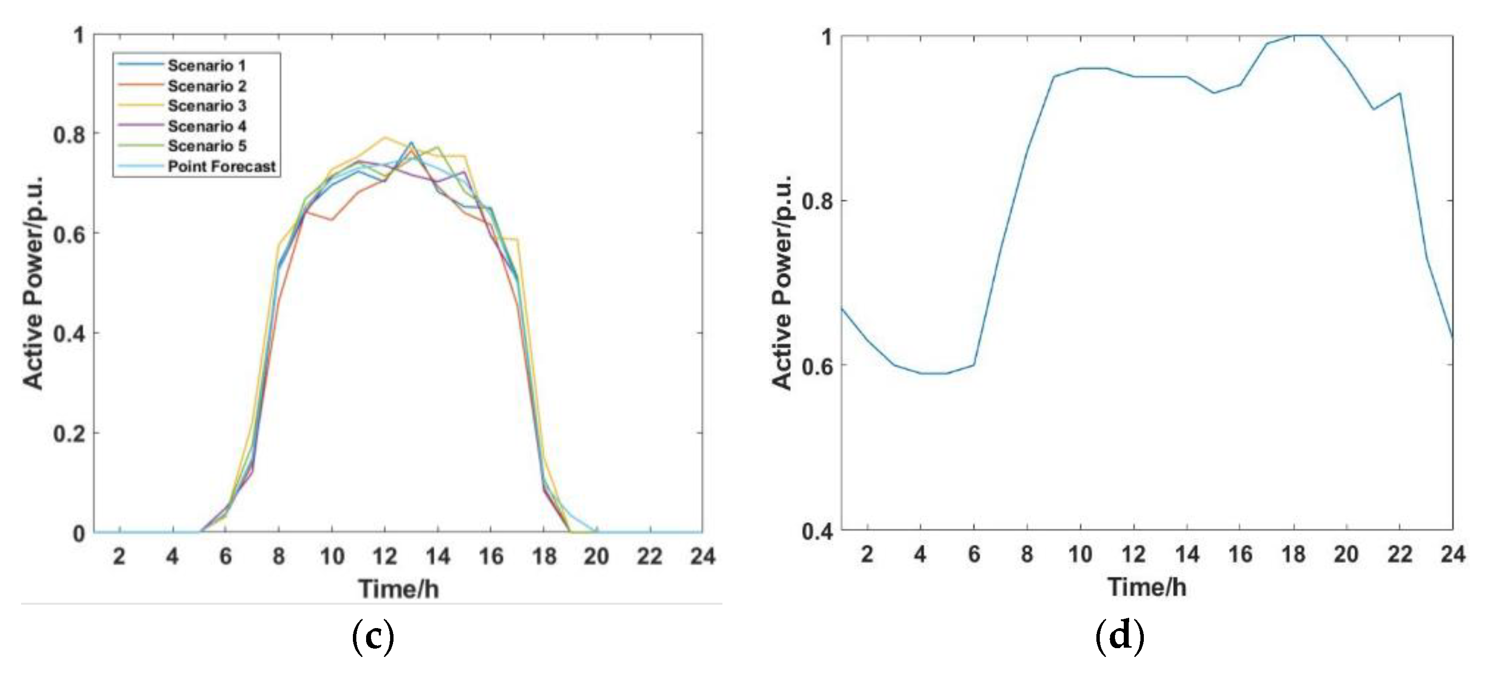
4.2.1. Probabilistic Renewable Energy Scenarios and the Load Power Forecast

The probabilistic renewable energy scenarios and the load power are illustrated in Figure 4. For the stochastic power forecasts of renewable energy, 5 scenarios are generated with a Latin hypercube sampling technique for utilization in the second stage model. The uncertainty of load is generally ignored in this paper, and the load is assumed to be independent from the renewable energy output. It is noted that the great uncertainty of stochastic renewable energy output and the large peak-valley difference of the expected load pose challenges to the power system operation.

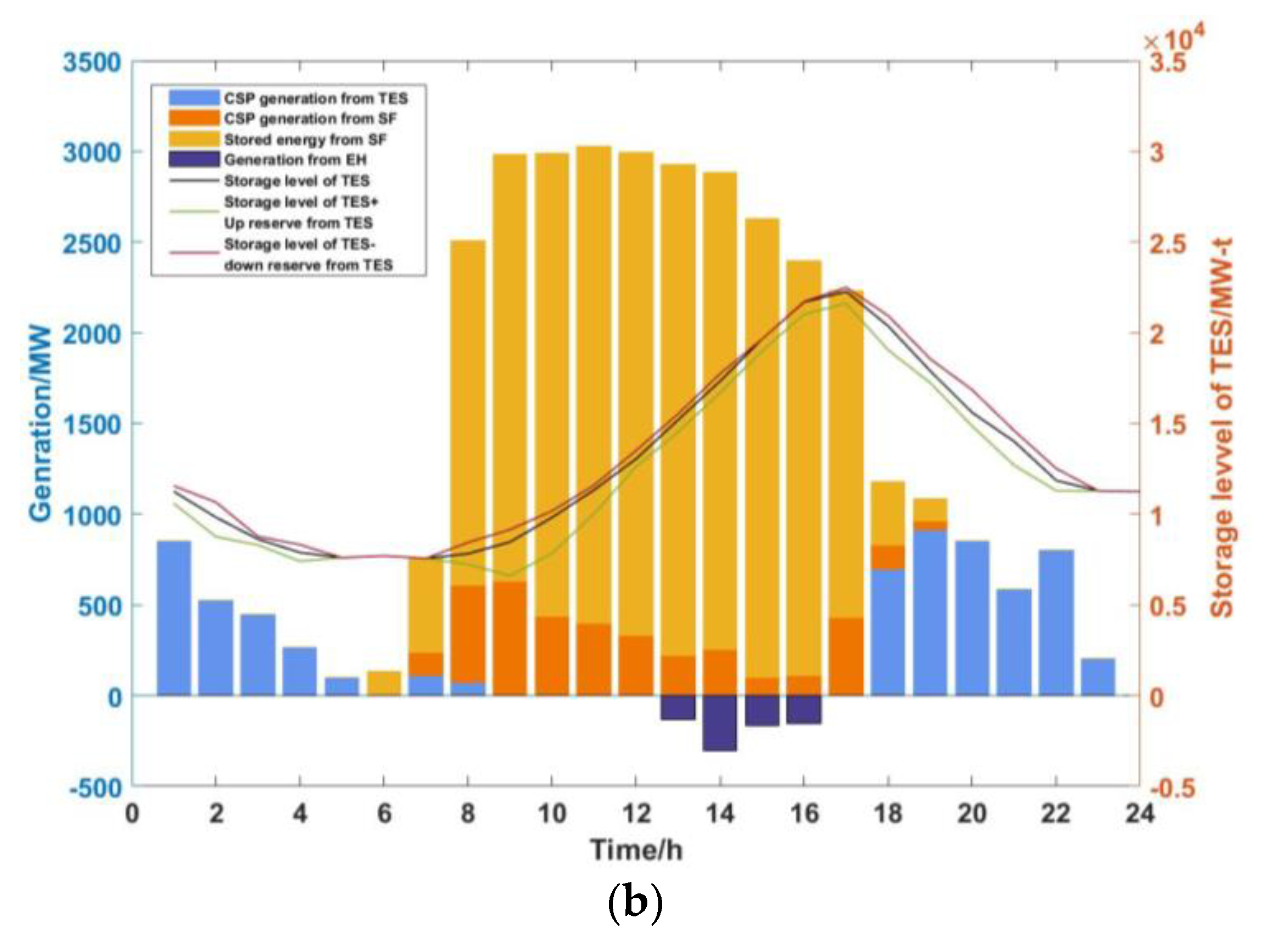
4.2.2. The Dispatch Results of the Multiple Resources with CSP and EH

The multiple generation system is composed of CSP, PV, wind power and traditional thermal units. EH is added to the CSP station, whose capacity is set as 50% of the CSP capacity.
The power dispatch results among the multiple resources are shown in Figure 5. Figure 5a illustrates the expected power generation of different generators. Figure 5b depicts the dispatch strategy of the TES system. The employment of TES turns CSP into a partially dispatched resource and the dispatchability of CSP is reflected in the following aspects. (1) At noon, when the illumination is rich and the power output of PV station is relatively high, the grid-connected CSP could decrease its output to around 0 (e.g., results from 12:00–16:00). In this time period, TES system is operated in the charging state to store the excess solar energy and EH is employed to absorb the surplus power generation from the gird for later use. (2) Correspondingly, when the power output of renewables is insufficient to meet the late peak period, CSP station could convert to the discharging state to maintain the power supply of CSP without light (e.g., results from 18:00–24:00). CSP could make up for the power vacancy and keep the power balance. (3) The fast ramp of traditional thermal units resulting from the fluctuation of load and renewables could be partially offset by the fast ramping rate of CSP. (e.g., results from 6:00–9:00 and 18:00–20:00).
Apart from the dispatchability of the CSP station, the additional functions of TES and EH could be demonstrated in two aspects which are clearly shown in Figure 5b. (1) TES could shift solar energy to periods of peak demand. Through adjusting the state of TES, the TES system could absorb solar energy from SF in the daytime, instead of generating electricity. The stored energy could be released when needed. The control strategy of the TES system guarantees the SOC of TES at the end of the day which supports the solar energy to be shifted between different days. The EH turns out to be the additional option for the better use of large-capacity of TES. (2) TES provides ancillary services like reserve services to cope with the uncertainty of renewables. From the storage level of TES system, it is recognized that the reserve capacity is not only determined by the reserve requirement but also the charging and discharging limits of TES, the up and down storage limits of TES and the ramping rate of the PB system.

4.2.3. The Unit Commitment Results Considering CSP and EH

Based on the proposed model concerning CSP and EH, the unit commitment solution is shown in Table 3, the system operating costs are shown in Table 4 and the CSP reserve planning results are illustrated in Figure 6.
The thermal unit 1, 2, 3, 5, 6, 7 and 8 with minor capacity of 76 MW have shut down in the test time period which decreases the fuel cost greatly, the other eight thermal units planning are listed in Table 3. The power vacancy arises from the reduced thermal units could be compensated by the CSP station and the increase CSP generating cost is compensated by the decline on fuel cost as shown in Table 4. Additionally, Table 3 records the fact that only four start-up processes happen to thermal unit 4 (76 MW), 10 (197 MW), 12 (155 MW) and 13 (155 MW) respectively. The less start-up times due to the flexibility of CSP with EH and the low start-up cost owing to the medium capacity of thermal units both lead to the reduction on system start-up cost illustrated in Table 4. Furthermore, the thermal unit 9 (350 MW), 14 (400 MW) and 15 (350 MW) with a large capacity keep working in the operating period to provide base-load capacity. At last, it is clear that the power system owns high reliability. The load shedding value is 0 which means that the power system with CSP and EH equipment has sufficient generating capacity to meet the peak load requirements at any time during the test period.
Figure 6a,b illustrate the results of the reserve planning in CSP station, including the overall scheduled up/down reserves in CSP stations and the actual reserve deployment in the stochastic scenario 3. Clearly, CSP is verified to provide reserve services owing to the employment of the large-capacity TES system. The optimized reserve solution could effectively reduce the economic cost by diminishing the up/down reserve during the valley load period. However, during the peak load period, more up reserves are provided to decrease the load shedding (e.g., results from 9:00–11:00 and results from 19:00–21:00). Meanwhile, the up reserve deployment and down reserve deployment could operate within the scheduled reserves. To sum up, the capability of the CSP station to provide reserve services could reduce the requirement of thermal unit reserve, thus promoting the penetration of renewable energy.

5. Discussion

In this section, in order to show the advantages of the proposed model, the comparison tests of the hybrid power system with different situations are given in the following part, in which the impacts on improving system flexibility through incorporating a CSP with TES/EH into the power system are analyzed from the perspective of energy services and reserve services. What’s more, the effectiveness of chance-constrained reserve planning is discussed in detail.

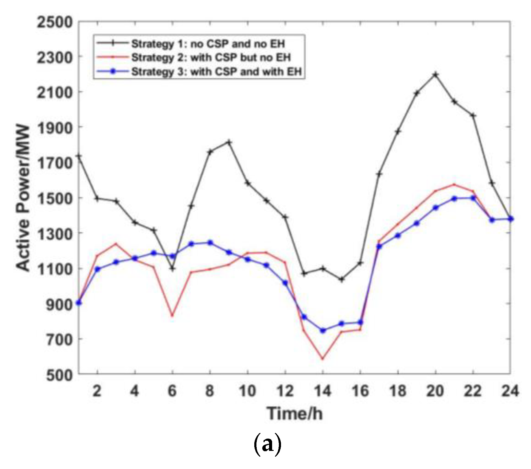
5.1. The Effects of CSP and EH in Energy Services

In this section, the effects of CSP and EH on the unit commitment and the influences on the renewables spillage are deeply considered in the comparison tests. Three strategies are involved in each tests. Strategy 1: no CSP and no EH; Strategy 2: with CSP but no EH; Strategy 3: with CSP and with EH.

5.1.1. The Influences of CSP and EH on Unit Commitment

Figure 7 shows the unit commitment decisions based on stochastic scenario 3.
In Strategy 1, thermal units are the only controllable resources to cope with the renewables uncertainty. The power output of thermal unit is constrained by the ramping limit, the operation space and the reserve requirement. It is noted in Figure 7a that thermal units need to ramp up quickly to counterbalance the decreased power output of the PV during the late peak hour. Therefore, as can be seen from Figure 7, in order to meet the power output constraints, large number of generators need to be turned on and operate at low power during abundant solar energy periods, creating the minimum generation constraint. The minimum generation constraint could be figured out as a flat line from 12:00 to 16:00 in Figure 7a. This operation not only increases the generation cost but also influences the penetration of renewable energy.
In Strategy 2, the dispatchable resource CSP is incorporated into the power system. Comparing Strategy 1 with Strategy 2 in Figure 7a–c, the conclusions could be summarized as follows. Firstly, as shown in Figure 5a and the related analysis, the solar power-driven PV and CSP station are complementary in their capability to serve different parts of load demand. It is noted in Figure 7a that the incorporation of the CSP could satisfy the load need in the late peak hour and thus the ramp rate and the range requirement of thermal units are reduced considerably from around 1200 MW to 800 MW in a few hours (16:00–20:00).
Secondly, as can be seen from Figure 7a, flexible CSP could reduce the minimum generator constraint from about 1100 MW in Strategy 1 to 800 MW in Strategy 2. In the short term, the reduction means that fewer thermal units need to operate at low power at noon, which is illustrated in Figure 7b,c. In the long term, the capability of CSP to provide firm capacity could potentially alternate the inflexible base load generating sets. The reduction of requirements for thermal units could accommodate greater utilization of renewables, and decrease the renewables spillage. The detailed comparison of renewables spillage is shown in Figure 8.
Finally, because of the power fluctuation of renewables, fast start-up and shut-down of the thermal units from 4:00 to 7:00 are worth noting in Strategy 1 as shown in Figure 7a,b. However, the incorporation of the CSP could smooth the power output of thermal units through controlling the large-capacity TES system. Therefore, the constant number of thermal units are needed in Strategy 2 which significantly reduces the start-up costs and has economic benefits.
In Strategy 3, the EH is equipped with a CSP station. From Figure 7a, the peak-valley difference in Strategy 3 is the minimum among the three strategies (Strategy 1: 1160 MW, Strategy 2: 986 MW, Strategy 3: 748 MW). During the daytime when the renewables resources are abundant and the electricity price is low, the EH equipment is employed to convert redundant power output to thermal energy stored in the TES for further use. Although the added EH would slightly increase the fuel costs of thermal units in the daytime, it could further utilize the room of the TES and decrease the generation cost and electricity cost during the late peak hour.

5.1.2. The Influences of CSP and EH on Renewables Curtailment

Figure 8 represents the effects of CSP and EH on the renewable energy curtailment considering different probabilistic scenarios. Figure 8a shows the capacity of generators in different penetrations, and the bar graphs in each penetration represent Strategy 1 to Strategy 3 successively. Wind power is 10% of the total capacity, CSP and PV share the same proportion, and EH is 50% of CSP capacity. Figure 8b illustrates the renewable energy curtailment rate in corresponding penetrations. The power spillage includes the surplus wind power, PV power and CSP power. In three strategies, the dotted line is the weighted average of renewable energy curtailment in Ns typical scenarios, where the weight coefficient can be determined through scenario probability. The solid line in each strategy represents the maximum value of renewable energy curtailment in Ns typical scenarios.
Comparing Strategy 1 with Strategy 2, it is clear that the average and maximum curtailment are significantly reduced owing to CSP station. For instance, when the renewables penetration is 20% in Strategy 1 (10% wind power and 10% PV), the curtailment reaches up to 36% (maximum) and 7.5% (average). However, when the renewable energy provides an additional 10% of the system energy in Strategy 2 (10% wind power, 10% PV and 10% CSP), the actual curtailment has dropped to less than 10% instead. Besides, CSP could effectively extend the feasible range of renewable energy penetration. In Strategy 1, without the CSP plant, 40% renewables penetration is the estimated upper limit of the scheduling model. In Strategy 2, although with the increasing renewables capacity, the ratio of renewable energy curtailment rises as well, the flexibility of the CSP makes the large-scale renewable energy penetration possible.
When an EH is added to the CSP plant, the operation of EH to reuse the surplus electricity contributes to the further curtailment reduction of renewables. Even with 90% penetration, the curtailment could be controlled under 30% (maximum). Therefore, the incorporation of a CSP with TES/EH could realize the 100% renewables-dominated power system.

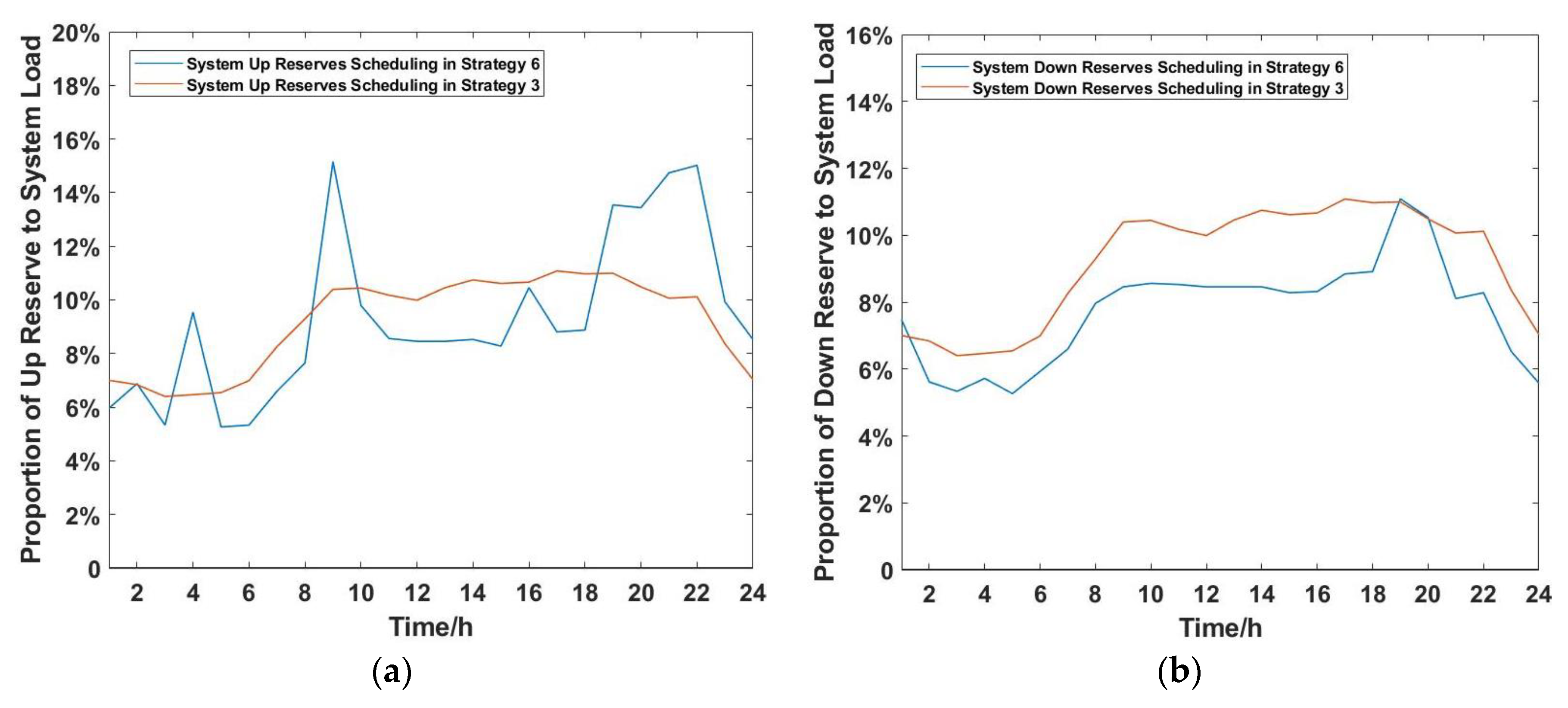
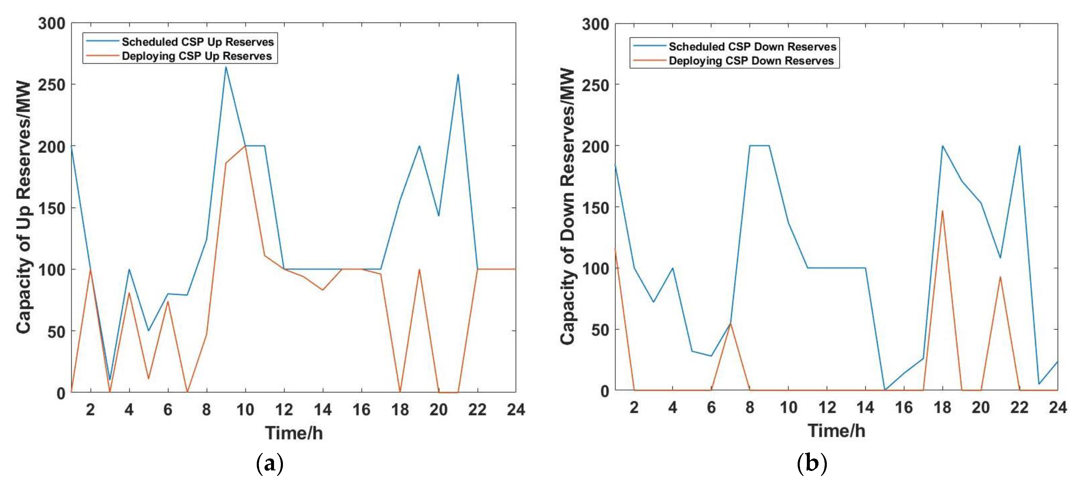
5.2. The Effects of CSP and EH in Reserve Services

5.2.1. Comparison Among Different Reserve Planning Decisions

In this section, 6 different spinning reserve strategies are formulated to discuss the advantages of the chance-constrained reserve planning model and the effects of the CSP and EH on the system costs. Different reserve strategies are depicted in Table 5. Table 6 shows the simulation results of the system costs based on different reserve strategy.
In Table 5 and Table 6, Strategy 1, Strategy 2 and Strategy 3 are the practical reserve planning methods with different system configurations while Strategy 4, Strategy 5 and Strategy 6 are the chance-constrained reserve planning with different system structures. In the comparative experiments of the conventional strategy and the proposed method, we could find that in the proposed chance-constrained manner, although the fuel costs, the start-up costs and the penalty costs for renewables spillage would increase, load shedding as the important criteria of system reliability would decrease significantly. Besides, the chance-constrained strategy effectively avoids consideration of extreme renewables fluctuation with low probability which reduces the costs for reserve scheduling and reserve deploying. Therefore, in the same system configuration, the system costs for chance-constrained programming are much lower than the traditional method.
To investigate the impacts of reserves from the CSP and EH on the system performance, different reserve settings are considered in the comparative experiments. In Strategy 2 and Strategy 4, CSP reserves are scheduled to replace part of the costly thermal unit reserves, and in Strategy 3 and Strategy 6, the EH is installed in the power system. The consideration of CSP reserves would slightly raise the fuel costs of thermal units, because the CSP energy to be released to the power system is now stored in TES to provide reserve services. The operation of the EH to absorb electricity from grid would further increase the fuel costs.
Whereas, the increase fuel costs are compensated by the decline on reserve costs. In the reserve scheduling process, CSP reserve is considered the best replacement of the costly thermal unit reserve which effectively minifies the requirement and the reserve scheduling cost of thermal unit reserve. In the reserve deploying process, inevitable deviations occur between the stochastic renewables power output and the scheduled value, and the deviations require more rapid response reserve deploying services. The CSP reserve deployment is constrained by the PB ramp rate and range (higher than the thermal units) and thus the reserve deploying costs decrease gently with CSP reserve services. The installation of an EH is the choice for the drop of reserve deploying costs, because the EH could respond quickly to mitigate the power output deviations instead of the unforeseen deployment of thermal unit reserve. Therefore, with the scheduling cost reduction by the CSP reserve and the deploying cost reduction by the EH equipment, the reserve costs are relatively low in Strategy 3 and Strategy 6.
In all, the chance-constrained reserve planning method with the consideration of reserve services from the TES/EH considered that the CSP station could achieve remarkable economic results.

5.2.2. Chance-Constrained Reserve Scheduling

Figure 9a,b show the total system reserves in Strategy 3 and Strategy 6, including CSP reserves and thermal units. It is clear that in Strategy 6, the optimized solution to the reserve scheduling demonstrates that during the valley of load demand, the reduced amount of scheduled reserves could decrease the system costs, and more reserves offered in the peak load hours could help reduce the probability of load shedding. The reduced requirement of system reserves in chance-constrained reserve planning increases the operating range of units and promotes the generation efficiency of the power system.

6. Conclusions

A CSP station turns out to be a dispatchable resource owing to the employment of the large-capacity TES and rapid response EH equipment. In this paper, a CSP is incorporated into a chance-constrained stochastic unit commitment model considering the economic and reliability criterion. The validity of the proposed model and the functions of the CSP and EH to provide energy and reserve services are tested in the IEEE reliability system.
Several conclusions are drawn as follows:
(1)
In the large-capacity renewables penetration system, the utilization of a TES and an EH could reduce the generation costs of thermal units and penalty costs for renewables spillage. The higher ramp rate and range of the CSP than thermal units support it to provide large scale of firm capacity. The reduced requirement of thermal units allows for greater renewables penetration. The EH enables the CSP to convert excess renewables generation into thermal units stored in TES for later use, which further utilizes the room of the TES system and reduces the renewables spillage significantly. The dispatchable CSP station with TES and EH makes a 100% renewable-dominated power system possible.
(2)
The reserve services provided by the CSP system with TES and EH could help decline the reserve costs. The capacity of CSP reserves mainly provides the reserve scheduling services through replacing expansive thermal unit reserves. The incorporation of an EH alleviates the renewables uncertainty to avoid unpredicted thermal unit reserve deployment.
(3)
In particular, the TES produces additional value by realizing the solar power shift to the periods of reduced power output and between different days. The complementary effects of solar-driven power CSP and PV stations enable greater use of solar energy especially in the high solar power penetrated power system.
(4)
Compared with a conventional reserve planning model, the proposed chance-constrained reserve scheduling has both economic value and reliable significance. The severe consequences of load shedding are greatly hedged in the proposed reserve planning method.
However, there were some limitations in this study. Firstly, the transmission expansion planning model was not considered in the stochastic unit commitment scheduling. In addition, the double-bounded property of wind power and PV power should be considered and the distribution function to describe limited variables like Beta distribution could be a more reasonable choice. Finally, we expect that the application of the proposed simulation framework into long-term planning could be carried out in a further study.

Author Contributions

Conceptualization, S.G., Y.Z. and Y.L.; Data curation, S.G.; Formal analysis, Y.L.; Investigation, Y.Z.; Methodology, Y.Z.; Project administration, S.G.; Resources, S.G.; Software, Y.Z.; Supervision, S.G. and Y.L.; Validation, S.G., Y.Z. and Y.L.; Visualization, Y.Z.; Writing—original draft, Y.Z.; Writing—review and editing, S.G. and Y.L.

Funding

This research was supported by “the Fundamental Research Funds for the Central Universities” in China.

Conflicts of Interest

The authors declare no conflict of interest.

Abbreviations

AbbreviationFull NameAbbreviationFull Name
CSPconcentrating solar powerDNIdirect normal irradiation
EDeconomic dispatchEENSexpected energy not supplied
EHelectrical heaterELNSexpected load not served
EWVSexpected wind and solar curtailmentFLHfull-load hour
HTFheat transfer fluidIEEEInstitute of electrical and electronics engineers
LSHLatin hypercube samplingLOLPloss-of-load probability
NP-Hardnon-deterministic polynomial hardPBpower block
PDFprobability distribution functionPVsolar photovoltaic
RTSreliability test systemSFsolar field
SMsolar multipleSOCstate of charge
TESthermal energy storageUCunit commitment

Appendix A

The McCormick convex envelope method (Big-M method) is utilized to linearize the NP-Hard problem. The technology is introduced below.
The bilinear terms in (41)–(44), (57)–(58) can be linearized using the following strategy. Let λ be continuous variable and σ be binary variable. The bilinear term λ σ can be formulated as follows.
μ = σ λ
Based on the Big-M technology, (A1) is rewritten in the following form.
{ M σ μ M σ M ( 1 σ ) + λ μ M σ
where, M is a sufficiently large number. The four constraints in (A2) are the equivalent linearized form of (A1). The analyses of (A2) are expressed as below: (1) If σ = 0, the first constraint guarantees μ = 0, and the second constraint always stands up. Therefore, σ = 0 means μ = 0. (2) If σ = 1, the second constraint guarantees μ = λ, and the first constraint always holds. Therefore, σ = 1 means μ = λ.

Appendix B

Table A1. Parameters of thermal units.
NumberTest Time/hScheduling Cost of Up Reserve/MWScheduling Cost of Down Reserve/MWDeploying Cost of Up Reserve/MWDeploying Cost of Down Reserve/MW
1761712027.270.00222
2761712027.270.00222
3761712027.270.00222
4761712027.270.00222
5761712027.270.00222
6761712027.270.00222
7761712027.270.00222
8761712027.270.00222
93502920017.920.00031
101972316016.60.002
111972316016.60.002
121552115019.70.00398
131552115019.70.00398
144003122016.190.00048
153502920017.920.00031
Table A2. Parameters of thermal units.
NumberCapacity/MWCoal Consumption CoefficientInitial State/hMinimum on Time/hMinimum off Time/hWarm Start Cost/MWCold Start Cost/MWMaximum Hot Start Time/h
a/MJb1/(MJ)b2/(MJ/MW·h)b3/(MJ/MW2·h)
1761712027.270.00222−111230046000
2761712027.270.00222−111230046000
3761712027.270.00222−111230046000
4761712027.270.00222−111230046000
5761712027.270.00222−111230046000
6761712027.270.00222−111230046000
7761712027.270.00222−111230046000
8761712027.270.00222−111230046000
93502920017.920.0003166610,00020,0004
101972316016.60.002−344550011,0002
111972316016.60.002−344550011,0002
121552115019.70.00398−333500010,0001
131552115019.70.00398−333500010,0001
144003122016.190.0004888812,50025,0005
153502920017.920.0003166610,00020,0004

References

  1. Du, E.S.; Zhang, N.; Hodge, B.M.; Wang, Q.; Kang, C.Q.; Kroposki, B.; Xia, Q. The Role of Concentrating Solar Power Toward High Renewable Energy Penetrated Power Systems. IEEE Trans. Power Syst. 2018, 33, 6630–6641. [Google Scholar] [CrossRef]
  2. Santosalamillos, F.J.; Pozovazquez, D.; Ruizarias, J.A. Combining wind farms with concentrating solar plants to provide stable renewable power. Renew. Energy 2015, 76, 539–550. [Google Scholar] [CrossRef]
  3. Chen, R.; Sun, H.B.; Guo, Q.L.; Li, Z.G.; Deng, T.H.; Wu, W.C.; Zhang, B.M. Reducing Generation Uncertainty by Integrating CSP With Wind Power: An Adaptive Robust Optimization-Based Analysis. IEEE Trans. Sustain. Energy 2019, 12, 583–594. [Google Scholar] [CrossRef]
  4. Kincaid, N.; Mungas, G.; Kramer, N. An optical performance comparison of three concentrating solar power collector designs in linear Fresnel, parabolic trough, and central receiver. Appl. Energy 2018, 231, 1109–1121. [Google Scholar] [CrossRef]
  5. Li, X.L.; Wang, Z.F.; Xu, E.S.; Ma, L.R. Dynamically Coupled Operation of Two-Tank Indirect TES and Steam Generation System. Energies 2019, 12, 1720. [Google Scholar] [CrossRef]
  6. Gafurov, T.; Prodanovic, M.; Usaola, J. Modelling of concentrating solar power plant for power system reliability studies. IET Renew. Power Gener. 2014, 9, 120–130. [Google Scholar] [CrossRef]
  7. Balghouthi, M.; Trabelsi, S.E.; Amara, M.B. Potential of concentrating solar power (CSP) technology in Tunisia and the possibility of interconnection with Europe. Renew. Sustain. Energy Rev. 2016, 56, 1227–1248. [Google Scholar] [CrossRef]
  8. Luo, Q.; Ariyur, K.B.; Mathur, A.K. Control-Oriented Concentrated Solar Power Plant Model. IEEE Trans. Control Syst. Technol. 2016, 24, 623–635. [Google Scholar] [CrossRef]
  9. Xu, T.; Zhang, N. Coordinated Operation of Concentrated Solar Power and Wind Resources for the Provision of Energy and Reserve Services. IEEE Trans. Power Syst. 2017, 32, 1260–1271. [Google Scholar] [CrossRef]
  10. Cocco, D.; Serra, F. Performance comparison of two-tank direct and thermocline thermal energy storage systems for 1 MWe class concentrating solar power plants. Energy 2015, 81, 526–536. [Google Scholar] [CrossRef]
  11. Manenti, F.; Ravaghiardebili, Z. Dynamic simulation of concentrating solar power plant and two-tanks direct thermal energy storage. Energy 2013, 55, 89–97. [Google Scholar] [CrossRef]
  12. Flueckiger, S.M.; Iverson, B.D.; Garimella, S.V.; Pacheco, J.E. System-level simulation of a solar power tower plant with thermocline thermal energy storage. Appl. Energy 2014, 113, 86–96. [Google Scholar] [CrossRef]
  13. Sioshansi, R.; Denholm, P. Benefits of Colocating Concentrating Solar Power and Wind. IEEE Trans. Sustain. Energy 2013, 4, 877–885. [Google Scholar] [CrossRef]
  14. He, G.; Chen, Q.; Kang, C.; Xia, Q. Optimal Offering Strategy for Concentrating Solar Power Plants in Joint Energy, Reserve and Regulation Markets. IEEE Trans. Sustain. Energy 2016, 7, 1245–1254. [Google Scholar] [CrossRef]
  15. Boland, J.; Cirocco, L.R.; Belusko, M.F.; Pudney, P. Controlling stored energy in a concentrating solar thermal power plant to maximise revenue. IET Renew. Power Gener. 2015, 9, 379–388. [Google Scholar]
  16. Kroposki, B.; Johnson, B.; Zhang, Y.C.; Gevorgian, V.; Denholm, P. Achieving a 100% Renewable Grid: Operating Electric Power Systems with Extremely High Levels of Variable Renewable Energy. IEEE Power Energy Mag. 2017, 15, 61–73. [Google Scholar] [CrossRef]
  17. Llamas, J.M.; Bullejos, D.; Ruiz de Adana, M. Optimal Operation Strategies into Deregulated Markets for 50 MWe Parabolic Trough Solar Thermal Power Plants with Thermal Storage. Energies 2019, 12, 935. [Google Scholar] [CrossRef]
  18. Chen, R.; Sun, H.; Li, Z.; Liu, Y. Grid Dispatch Model and Interconnection Benefit Analysis of Concentrating Solar Power Plants with Thermal Storage. Autom. Electr. Power Syst. 2014, 38, 1–7. [Google Scholar]
  19. Du, E.S.; Zhang, N.; Hodge, B.M.; Wang, Q.; Kang, C.Q.; Kroposki, B.; Xia, Q. Operation of a High Renewable Penetrated Power System With CSP Plants: A Look-Ahead Stochastic Unit Commitment Model. IEEE Trans. Power Syst. 2019, 34, 140–151. [Google Scholar] [CrossRef]
  20. Wagner, M.J.; Newman, A.M.; Hamilton, W.T.; Braun, R.J. Optimized dispatch in a first-principles concentrating solar power production model. Appl. Energy 2017, 203, 959–971. [Google Scholar] [CrossRef]
  21. Pozo, D.; Contreras, J. A chance-constrained unit commitment with an n-k security criterion and significant wind generation. IEEE Trans. Power Syst. 2013, 28, 2842–2851. [Google Scholar] [CrossRef]
  22. Luo, Y.; Lu, T.; Du, X.Z. Novel optimization design strategy for solar power tower plants. Energy Convers. Manag. 2018, 177, 682–692. [Google Scholar] [CrossRef]
  23. Wu, H.; Shahidehpour, M.; Li, Z. Chance-constrained day ahead scheduling in stochastic power system operation. IEEE Trans. Power Syst. 2014, 29, 1583–1591. [Google Scholar] [CrossRef]
  24. Du, E.S.; Zhang, N.; Kang, C.; Xia, Q. Scenario Map Based Stochastic Unit Commitment. IEEE Trans. Power Syst. 2018, 33, 4694–4705. [Google Scholar] [CrossRef]
  25. Boukelia, T.E.; Mecibah, M.S.; Kumar, B.N.; Reddy, K.S. Investigation of solar parabolic trough power plants with and without integrated TES (thermal energy storage) and FBS (fuel backup system) using thermic oil and solar salt. Energy 2015, 88, 292–303. [Google Scholar] [CrossRef]
  26. Fernández-García, A.; Rojas, E.; Pérez, M.; Silva, R.; Hernández-Escobedo, Q.; Manzano-Agugliaro, F. A parabolic-trough collector for cleaner industrial process heat. J. Clean. Prod. 2015, 89, 272–285. [Google Scholar] [CrossRef]
  27. Pousinho, H.M.I.; Silva, H.; Mendes, V.M.F. Self-scheduling for energy and spinning reserve of wind/CSP plants by a MILP approach. Energy 2014, 78, 524–534. [Google Scholar] [CrossRef]
  28. Zhang, Y.; Wang, J.; Wang, X. Review on probabilistic forecasting of wind power generation. Renew. Sustain. Energy Rev. 2014, 32, 255–270. [Google Scholar] [CrossRef]
  29. Ma, X.; Sun, Y.; Fang, H. Scenario Generation of Wind Power Based on Statistical Uncertainty and Variability. IEEE Trans. Sustain. Energy 2013, 4, 894–904. [Google Scholar] [CrossRef]
  30. Shen, Y.X.; Wang, X.; Chen, J. Wind Power Forecasting Using Multi-Objective Evolutionary Algorithms for Wavelet Neural Network-Optimized Prediction Intervals. Appl. Sci. 2018, 8, 184–196. [Google Scholar]
  31. Yang, M.; Lin, Y.; Han, X. Probabilistic Wind Generation Forecast Based on Sparse Bayesian Classification and Dempster–Shafer Theory. IEEE Trans. Ind. Appl. 2016, 52, 1998–2005. [Google Scholar] [CrossRef]
  32. Dale, M.A. Comparative Analysis of Energy Costs of Photovoltaic, Solar Thermal, and Wind Electricity Generation Technologies. Appl. Sci. 2013, 3, 325–337. [Google Scholar] [CrossRef]
  33. Wang, J.; Botterud, A.; Bessa, R.; Keko, H.; Carvalho, L.; Issicaba, D.; Sumaili, J.; Miranda, V. Wind power forecasting uncertainty and unit commitment. Appl. Energy 2011, 88, 4014–4023. [Google Scholar] [CrossRef]
  34. Mazzeo, D.; Oliveti, G.; Labonia, E. Estimation of wind speed probability density function using a mixture of two truncated normal distributions. Renew. Energy 2018, 115, 1260–1280. [Google Scholar] [CrossRef]
  35. Cordova, S.; Rudnick, H.; Lorca, A.; Martinez, V. An Efficient Forecasting-Optimization Scheme for the Intra-Day Unit Commitment Process Under Significant Wind and Solar Power. IEEE Trans. Sustain. Energy 2018, 99, 1899–1909. [Google Scholar] [CrossRef]
  36. Ascione, F.; Bianco, N.; Stasio, C.D.; Mauro, G.M.; Vanoli, G.P. Full text access Multi-stage and multi-objective optimization for energy retrofitting a developed hospital reference building: A new approach to assess cost-optimality. Appl. Energy 2016, 174, 37–68. [Google Scholar] [CrossRef]
  37. Tan, S.M.; Wang, X.; Jiang, C.W. Optimal Scheduling of Hydro–PV–Wind Hybrid System Considering CHP and BESS Coordination. Appl. Sci. 2019, 9, 892. [Google Scholar] [CrossRef]
  38. Lu, Z.W.; Wu, C.D.; Yu, X.S. Learning Weighted Forest and Similar Structure for Image Super Resolution. Appl. Sci. 2019, 9, 543. [Google Scholar] [CrossRef]
  39. Wu, Z.; Liu, P.X.; Gu, W. A bi-level planning approach for hybrid AC-DC distribution system considering N-1 security criterion. Appl. Energy 2018, 230, 417–428. [Google Scholar] [CrossRef]
  40. Mirzaei, M.A.; Yazdankhah, A.S.; Mohammadi-Ivatloo, B.; Marzband, M.; Shafie-khah, M.; Catalão, J.P. Stochastic network-constrained co-optimization of energy and reserve products in renewable energy integrated power and gas networks with energy storage systems. J. Clean. Prod. 2019, 223, 747–758. [Google Scholar] [CrossRef]
  41. Papavasiliou, A.; Oren, S.S.; O’Neill, R.P. Reserve requirements for wind power integration: A scenario-based stochastic programming framework. IEEE Trans. Power Syst. 2011, 26, 2197–2206. [Google Scholar] [CrossRef]
  42. Löfbergi, J. Available online: http://users.isy.liu.se/johanl/yalmip/pmwiki.php?n=Ma (accessed on 20 March 2019).
  43. Reliability Test System Task Force of the Application of Probability Methods Subcomittee. IEEE reliability test system. IEEE Trans. Power App. Syst. 1979, 98, 2047–2054. [Google Scholar]
  44. Praveen, R.P.; Baseer, M.A.; Awan, A.B.; Zubair, M. Performance Analysis and Optimization of a Parabolic Trough Solar Power Plant in the Middle East Region. Energies 2018, 11, 741. [Google Scholar] [CrossRef]
  45. Gong, Y.; Chung, C.Y.; Mall, R.S. Power System Operational Adequacy Evaluation with Wind Power Ramp Limits. IEEE Trans. Power Syst. 2018, 33, 2706–2716. [Google Scholar] [CrossRef]
  46. Shouman, E.R.; Khattab, N.M. Future economic of concentrating solar power (CSP) for electricity generation in Egypt. Renew. Sustain. Energy Rev. 2015, 41, 1119–1127. [Google Scholar] [CrossRef]
  47. Dominguez, R.; Baringo, L.; Conejo, A.J. Optimal offering strategy for a concentrating solar power plant. Appl. Energy 2012, 98, 316–325. [Google Scholar] [CrossRef]
  48. Heydarian-Forushani, E.; Golshan, M.E.H.; Shafie-khah, M. Flexible security-constrained scheduling of wind power enabling time of use pricing scheme. Energy 2015, 90, 1887–1900. [Google Scholar] [CrossRef]
Figure 1. Configuration of a two-tank concentrating solar power (CSP) station with electrical heater (EH) equipment.
Applsci 09 02340 g001
Figure 2. Simplified energy flow in CSP station with thermal energy storage (TES) and EH.
Applsci 09 02340 g002
Figure 3. Load shedding and renewable energy spillage.
Applsci 09 02340 g003
Figure 4. Point forecast and scenario-based probabilistic forecast containing: (a) wind power forecast; (b) PV forecast; (c) CSP solar thermal power forecast; (d) load demand.
Applsci 09 02340 g004aApplsci 09 02340 g004b
Figure 5. The power dispatch results including: (a) the coordinated operation of the multiple resources; (b) the dispatch strategy of the TES system.
Applsci 09 02340 g005aApplsci 09 02340 g005b
Figure 6. CSP reserve planning results at stochastic scenario 3, including: (a) the total scheduled up reserves and reserve deployment in CSP stations; (b) the total scheduled down reserves and reserve deployment in CSP stations.
Applsci 09 02340 g006
Figure 7. Unit commitment results in three strategies: (a) the power supply of traditional thermal units; (b) the generation schedule of thermal units; (c) the number of thermal units turned on.
Applsci 09 02340 g007aApplsci 09 02340 g007b
Figure 8. Capacity and curtailment of renewable energy assuming an equal mix of PV and CSP in three strategies, including (a) the capacity of generators in different penetrations; (b) the renewable energy curtailment rate in different penetrations.
Applsci 09 02340 g008
Figure 9. CSP and system reserve planning results at stochastic scenario 3, including: (a) the total scheduled system up reserves in Strategy 3 and Strategy 6; (b) the total scheduled system down reserves in Strategy 3 and Strategy 6.
Applsci 09 02340 g009
Table 1. Capacity of generators in the modified 24-bus IEEE reliability power system.
LoadThermal UnitCSPPVWind Power
Quality/N1715333
Total Capacity/MW2850241215001500900
Table 2. Parameters of CSP station.
ParameterValueParameterValue
P c P B , u p , P c P B , d n 50% P c P B , m a x Initial State of Charge (SOC)50% E c T E S , +
T c , m i n P B , o n , T c , m i n P B , o f f 2(h) E c P B , s t 50 MW−t
Solar Multiple (SM)2.4 η c P B 38%
Full-load Hour (FLH)15(h) η c T E S , c h a , η c T E S , d i s 98%
γ c T E S 0.003 R c P B , u p , + , R c P B , d n , + 30% P c P B , m a x
Table 3. Unit commitment solution for the stochastic model.
Time/hThermal Unit Number
49101112131415
111111111
211111111
311111111
411111111
511111111
611111111
711111111
811111111
911111111
1011111111
1111111111
1211111111
1311010011
1411010011
1501010011
1611010011
1711111111
1811111111
1911111111
2011111111
2111111111
2211111111
2311111111
2411111111
Table 4. Results for system costs with CSP and EH equipment.
System Operating Costs ($)Value
Fuel cost558,906.38
Start-up cost2300
Generating cost for CSP and EH50,701.16
Penalty cost for load shedding0.00
Penalty cost for renewables spillage1432.59
Cost for thermal unit reserve scheduling13,756.84
Cost for thermal unit reserve deploying1717.01
Total system cost644,287.84
Table 5. Different reserve strategies.
Strategy Description
Strategy 1Reserve adopts 10% of load forecast + additional 5% of wind forecast
No CSP reserve, and no EH
Strategy 2Reserve adopts 10% of load forecast + additional 5% of wind forecast
With CSP reserve, but no EH
Strategy 3Reserve adopts 10% of load forecast + additional 5% of wind forecast
With CSP reserve, and with EH
Strategy 4Reserve adopts chance-constrained programming
No CSP reserve, and no EH
Strategy 5Reserve adopts chance-constrained programming
With CSP reserve, but no EH
Strategy 6Reserve adopts chance-constrained programming
With CSP reserve, and with EH
Table 6. Simulation results of system costs based on different reserve strategy.
StrategyFuel Costs and Start-Up Costs ($)Penalty Costs for Load Shedding ($)Penalty Costs for Renewables Spillage ($)
Strategy 1607,959.732005.35129.12
Strategy 2609,017.211705.31 2153.51
Strategy 3610,477.49179.29 1274.90
Strategy 4610,624.39197.556006.07
Strategy 5611,379.23161.182715.00
Strategy 6611,907.540.00 1432.59
StrategyCosts for Reserve Scheduling ($)Costs for Reserve Deploying ($)System Costs ($)
Strategy 139,615.546572.71704,195.06
Strategy 216,363.145575.36660,028.64
Strategy 314,402.792177.49645,092.24
Strategy 424,599.495846.88674,393.30
Strategy 515,963.144721.84658,952.82
Strategy 613,756.841717.01644,287.84

