Article

Empirical Evidences for Urban Influences on Public Health in Hamburg

1
Department of Geography, Universität Hamburg, 20146 Hamburg, Germany
2
Department of Geography, Ruhr-Universität Bochum, 44799 Bochum, Germany
3
Faculty of Medicine, Ruhr-Universität Bochum, 44801 Bochum, Germany
*
Author to whom correspondence should be addressed.
Appl. Sci. 2019, 9(11), 2303; https://doi.org/10.3390/app9112303
Submission received: 22 March 2019 / Revised: 30 April 2019 / Accepted: 31 May 2019 / Published: 4 June 2019
(This article belongs to the Special Issue New and Old Environmental Impacts on Population Well Being)

Abstract

:
From the current perspectives of urban health and environmental justice research, health is the result of a combination of individual, social and environmental factors. Yet, there are only few attempts to determine their joint influence on health and well-being. Grounded in debates surrounding conceptual models and based on a data set compiled for the city of Hamburg, this paper aims to provide insights into the most important variables influencing urban health. Theoretically, we are primarily referring to the conceptual model of health-related urban well-being (UrbWellth), which systemizes urban influences in four sectors. The systematization of the conceptual model is empirically confirmed by a principal component analysis: the factors derived from the data correspond well with the deductively derived model. Additionally, a multiple linear regression analysis was used to identify the most important variables influencing the participant’s self-rated health (SRH): rating of one’s social network, rating of neighborhood air quality, rating of neighborhood health infrastructure, heat stress (day/outdoors), cold stress (night/indoors). When controlling for age, income and smoking behavior, these variables explain 12% of the variance of SRH. Thus, these results support the concept of UrbWellth empirically. Finally, the study design helped to identify hotspots with negative impact on SRH within the research areas.

1. Introduction

1.1. Conceptions of Urban Health and Research Design

On a rapidly urbanizing planet, health and well-being in urban areas are of particular concern. While urban dwellers in general do quite well and have higher life expectancy in particular [1], there are also drawbacks of life in cities [2]. Most importantly, urban areas face multiple environmental challenges, such as heat, noise, and pollutants [3]. The joint effects of these multiple stressors can have a large impact on the quality of life and health of the inhabitants. Thus, health in urban areas is receiving increasing attention, which requires a clarification of the concepts of health and well-being and an understanding of the influences exerted by the urban environment.
In public health research, health in urban areas is understood as being affected by a large variety of variables [4,5,6,7]. From the 1980s onwards, ecological models have been developed [8,9]; these have been extended with regard to the influence of lifestyle [10], political context [11], or in connection to ecosystem services [12].
Our research design was developed in relation to this discussion and is also related to the so-called ecological turn in health-related research of urban well-being [13,14,15]. Following Cummins et al. (2007), we are interested in the interrelationships between individual characteristics, lifestyles and behavior, on the one hand—factors which may characterize individual exposures—and place-based environmental contexts, on the other hand—factors leading to social exposures [16]. There have already been several attempts to conceptualize these complex interrelations for urban areas [17,18]. Additionally, differences in health systems can result in great geographical variation in health outcomes [19,20].
One starting point of these concepts was the thesis of an “underrepresentation” of place effects and urban influences on health in traditional health research [21]. The WHO also suggests a more holistic understanding of health: following a salutogenic approach, health is defined as “the state of complete physical, mental and social well-being and not just the absence of illness or infirmity” [22]. This resource-based concept of health captures a person’s ability to respond to external and internal stressors. This basic attitude of the individual is referred to in Antonovsky’s salutogenesis model as a “sense of coherence” [23].
To investigate this more holistic conception of health, health-related quality measures (HRQOL) have been developed in health research and used as an endpoint in clinical trials. Various instruments have been developed for measuring HRQOL [24,25,26]. Self-rated health (SRH) is a stronger predictor of mortality and morbidity than many objective measures of health, for example [27,28]. Thus, the prevalence of cardio-cerebral vascular diseases, for example, is associated with poorer SRH [29]. Therefore, SRH is suitable as a basis for the investigation of health-related well-being, analyzed in this paper.
Szombathely et al. have presented a current overview of the development of the concepts of health in urban health research [30]. Based on this review, a conceptual model of health-related urban well-being (UrbWellth) has been elaborated that differs from existing approaches mainly in the analytical distinctions it suggests. The model introduces well-being [31,32] as the target value. Figure 1 shows a simplified version of the model of UrbWellth in order to present the general ideas behind the systematization of UrbWellth relevant to the analyses in this paper.
Issues of human-environmental relations are addressed through a basic binary structure (citizens—urban environment), suggested in several other Public Health models [8,10,33]. Additionally, this binary view was subdivided into four sectors: individual and society for the citizens, morphology and stressors for the urban environment, to proceed to a detailed understanding of the city’s internal relations. The individual sector includes socio-economic and selected behavioral variables and predispositions [34,35] and therefore also the most important confounding variables from epidemiology and health research perspectives [17,36,37,38]; the society sector comprises security, activity patterns and class/lifestyle [9,39]. Urban morphology encompasses the provision of services, which can be assessed in the sense of an urban ecosystem [40]; it does not distinguish between the natural and the built environment. The stressors include noise, thermal stressors, and air quality [41,42,43].

1.2. Selected Empirical Results and Research Gaps

According to the definition above, health is not solely the result of individual factors; social factors need to be considered [44]. This can be explained by using the example of housing. Krieger and Higgins found that living space “can influence both physical and mental health, including asthma and other respiratory conditions, injuries, psychological distress, and child development” [45]. However, research on housing and health focused primarily on the physical aspects of housing, such as the building conditions [46], while social drivers may have gone undetected. Additionally, the effects of housing on health depend on a third variable: exposure to environmental stressors, which cannot be analyzed without considering social stratification [47]. Therefore, the conception of public health needs to be accompanied by an understanding of the production of stratification [48,49,50] of a city’s society [30], a context that needs to be in focus in public health research.
Exposure to road traffic noise and aircraft noise—also dependent on social characteristics—was associated with different cardiovascular diseases [51,52,53], respiratory diseases [54,55], and depression and anxiety [56,57]. Other studies investigated exposure to air pollution and found higher risk for all causes and cardio-respiratory mortality [58,59,60,61]. Comparatively little is known about the effect of air pollution on depressive symptoms or anxiety [62,63]. Empirical research shows that urban green and blue areas have a positive effect on mental health [64] and a sense of coherence and mental health are closely related [65,66]. Yet, the link to physical health is less clear.
The consequences of thermal conditions for health are often evaluated using thermal indices to calculate the impact of the thermal environment on humans [67,68,69]. Epidemiological studies found for numerous cities that mortality increases during periods of extreme heat stress, as well as during periods of cold stress [70,71,72]. The connection to SRH has not been studied so far.
Additionally, confounders such as gender, age or income, and behavioral variables such as smoking status, alcohol consumption, or physical activity have to be taken into account as effect-modifying variables [34,35,47,73]. Access to healthcare and social support play a role in specific health outcomes and should be considered in studies as well [8,74,75,76]. The relationship with SRH is the focus of this investigation.

1.3. Research Questions

The conceptual model and the variety of variables which are included lead to two interrelated questions: how can multi-influences or -stressors for urban SRH be determined by means of a linear regression model? Which variables have the greatest influence and how are they distributed geographically? Especially, urban influences are to be identified. Answers to these questions will be presented as an empirical case study based on the model of UrbWellth, designed to test the conceptual ideas, systemize the results, identify the most important variables and address further open questions.

2. Materials and Methods
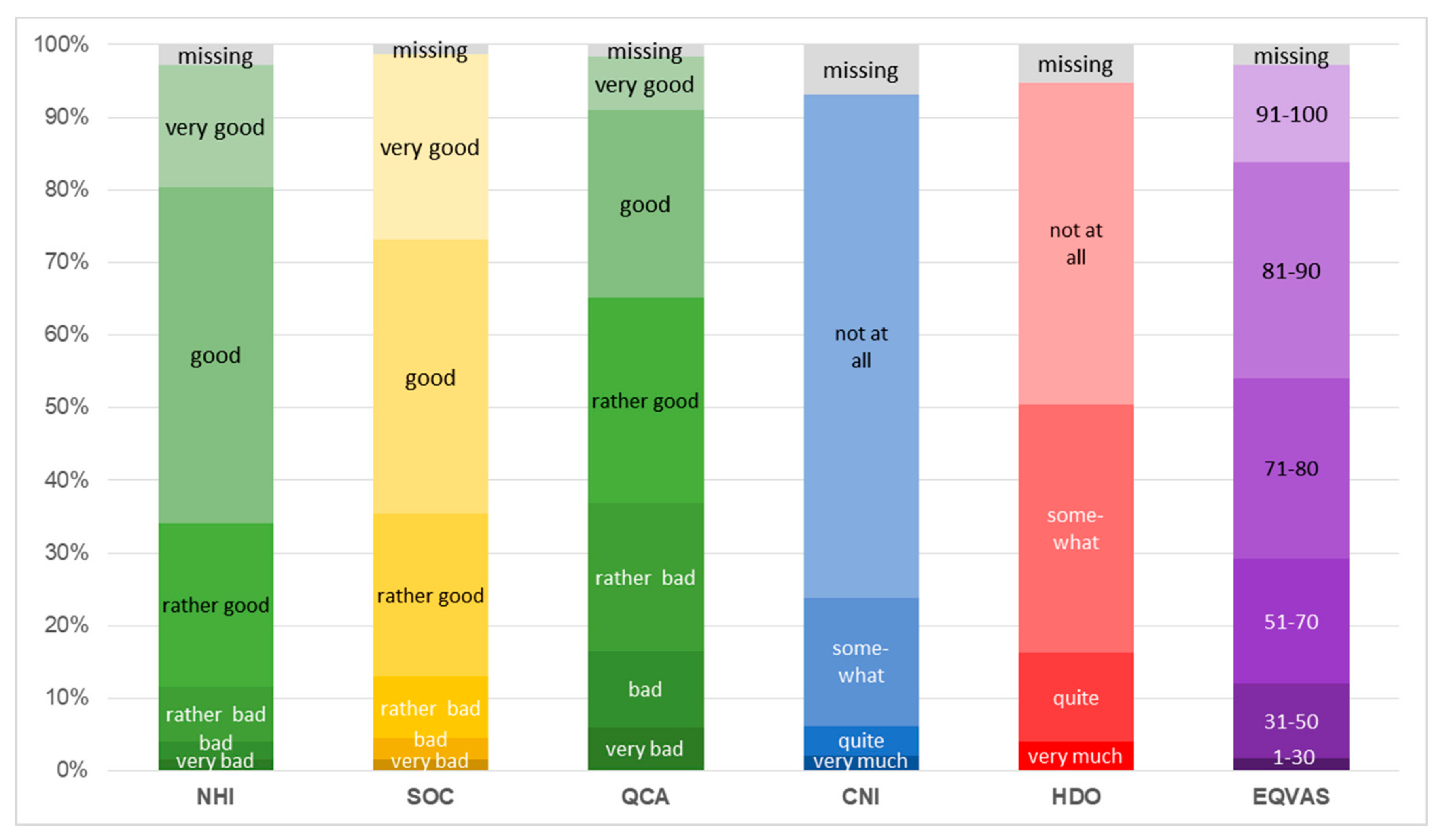
2.1. Data Collected

There are hardly any high-resolution data sets that link georeferenced health data with socio-demographic data in Hamburg. Thus, we conducted a household survey to collect primary data with a spatial resolution of urban blocks [77]. The variables for this data collection were derived from the UrbWellth model [30]. In addition, various health-related assessment tools were evaluated [32,78,79,80,81] to inform our questionnaire. When selecting the study areas in Hamburg (see Figure 5), small-scale differences in socio-economic burden [82], exposure to noise [83], and temperature [84] were taken into account [77]. Air quality was not considered since fine scale exposure cannot be observed without huge effort and there is no high-resolution data set available for air pollution in Hamburg. The survey areas were to cover the city’s spatial extent and depict different district types derived from urban morphology, because urban morphology was used as a proxy for the structural quality of buildings, a general vulnerability assessment, and the local micro-climate [85,86].
Questions about living conditions and assessments of the residential area (satisfaction with infrastructure and assets, future wishes), mobility behavior (transport used, duration, reasons for use), subjective health assessment [32,87], and environmental pollution stressors were included. The final survey also included questions on socio-economic characteristics (education, income, occupation, age, etc.). The questionnaires comprised a total of 51 questions and were hand-delivered into residential mail boxes in 24 study areas. One person above 18 years old per household was asked to respond and return the survey by the postage-paid return envelope within two weeks. The questionnaires were distributed in November 2016 and April 2017; thus, a direct influence of extreme weather events (heat or cold wave) on the survey results could be avoided. The complete questionnaire is available from the authors.
Each study area comprised between 150 and 400 households (6620 total). A total of 1081 surveys were returned. The participation rate of 16.24% was below the response rates for similar surveys, which can be explained by the lack of a reminder, itself resulting from a lack of resources. The differences between the survey areas are high (the response rates varied from 3.1% to 43.5%). In general, the highest response rates were achieved in areas of high socioeconomic status, and the lowest rates corresponded to those with low socioeconomic status.
Most questions were answered using four- to six-point Likert scales (depending on the topic and the use of existing instruments, see Table 1). Nonetheless, some questions were answered on a binary scale or were open. Thus, not all of the survey’s questions were used for the analyses in this paper. The questions pertaining to assessments of subjective health are based on the EQ-5D-5L, “a standardized non-disease specific instrument to describe and value health-related quality of life” [88] developed by EuroQol Group in 1987. The instrument is divided into the EQ-5D descriptive system which comprises the categories of mobility, self-care, daily activities, pain/discomfort, anxiety/depression and the EQ visual analogue scale (EQ VAS), marking self-related health on a scale (0–100). In the questionnaire, one question was assigned to each descriptive category, using EuroQol’s levels ranging from “no problems” to “extreme problems” as potential answers (see Table 1). A further question refers to the EQ VAS by prompting participants to judge their current health on a scale from 0 to 100 from worst to best [89].
All other questions were either derived from the UrbWellth model directly or derived from one of the other surveys evaluated [32,78,79,80,81]. The whole questionnaire was pre-tested several times (12 participants in total). Answers on paper were then digitized into the package SPSS 24 (IBM). From the 51 questions 152 variables were derived (single questions led to up to 12 variables) [77]. Only some questions of the questionnaire were used in this study (Table 1).

2.2. Methods and Statistical Tests

SPSS 24 was used for all statistical analyses. The total number of variables used for the principal component analysis (PCA) is 41, representing the survey questions described in Section 2.1, which could be included in the analyses according to their type of question or answer scale. We chose an explorative PCA for two reasons. The primary purpose was to test the conceptual systematization of the UrbWellth model. Secondly, all variables connected to the subjective rating of health were to be identified, guiding the selection of independent variables for the linear regression model (LR), which is our second main analysis method (see Section 3.2). All variables of the principal component “health” (including SRH) were excluded from the list of independent variables in the LR. Subsequently a LR was conducted to identify the most important variables that impact SRH and to model the respective influence of each of these variables.
There are some general requirements that should be met for a PCA. Firstly, the relationship between the variables should be linear. Secondly, the certainty of the results depends on the sample size [90]. Both these criteria are met by our data (see Section 3.1). Thirdly, the variables should be continuous, although ordinal data are often used [91]. Lastly, there should be no outliers in the data. These last two criteria are only partly fulfilled by our data. We have countered this by excluding individual variables that did not match these requirements.
Table 1 gives an overview of the variables used. The first column provides a number, used as an ID; the second column shows the content of the questions. The third column introduces abbreviations which will be used throughout the paper when referring to specific variables. Column four provides the number of valid cases (N) ranging from 953 to 1077, followed by Mean, Min, Max, and standard deviation (SD). Additional information on the type of answer scale and the answering options available is given in column five, comprising different numbered types.
The main prerequisite for the multiple LR is that the data exist on an ordinal scale that is also considered an interval scale (assumption: equal distances between the classes). Further requirements are a linear relationship between the variables, no outliers in the data, independence of the error terms, a check for multicollinearity, and homoscedasticity and a normal distribution of the residuals. These prerequisites have either been met or, in the course of the analysis, the necessary steps have been taken to fulfill them: a leverage test was carried out to identify outliers. When using the limiting value of 0.2 or higher suggested by Huber [92], no values had to be classified as outliers, but the test by Velleman and Welsch [93] resulted in the exclusion of three values as outliers. Calculating Cook’s distance did not identify outliers, as all values remain below the cut-off value of 1.
The model has no auto-correlation, as the value of the Durbin–Watson statistic is 2.056. Pearson correlation remains clearly below 0.3 and all tolerance values are around 0.9; thus, no multicollinearity is to be expected. Due to homoscedasticity tests, the model can be assumed to equally predict values throughout all variables depicted. Histograms of the standardized residuals illustrate an approximately normal distribution produced by the model. The P-P-diagram also depicts a distribution of the data that is close to normal distribution; LR is therefore possible.

3. Results: Identifying Urban Influences on Health

3.1. Principal Component Analysis

A principal component analysis (PCA) was conducted to obtain a data-based systematization of the variables and to inform the linear regression model (LR). It was ensured that all items correlated to the degree of at least 0.3 with at least one other item. The Kaiser–Meyer–Olkin measure of sampling adequacy is 0.84, therefore clearly above the commonly recommended value of 0.6. Bartlett’s test of sphericity is significant (x2 (829) = 11,274.435, p < 0.01). The diagonals of the anti-image correlation matrix are all over 0.5, and the communalities are all above 0.3, further confirming that each item shares some common variance with other items. Given these results, factor analysis was decided to be suitable with all 41 items selected.
Initial eigenvalues for the first three components explained 19%, 9%, and 7% of the variance respectively, with eigenvalues of 3% to 7.7%. The fourth to 12th factors had eigenvalues above one, and each explained 2.5% to 4.7% of the variance. Solutions for three to 12 factors were each examined using Quartimax rotation of the factor loading matrix. The nine-factor solution, which explained 59% of the variance, was preferred because of: (a) the goal of achieving a variance elucidation of >60% using the defined factors; (b) examination of the scree plot; and (c) the ninth factor was the last factor to explain more than 3% of the variance. No items were eliminated because all items contribute to a simple factor structure and meet a minimum criterion of having a primary factor loading of 0.37 or above. The factor loading matrix for this solution is presented in Table 2.
The factor labels were deducted from the variables assigned to the factors. Internal consistency for each of the scales was examined using Cronbach’s alpha. Cronbach’s alpha for factor 1 (Environmental qualities, infrastructure and security) is 0.889 (12 items), which indicates a high level of internal consistency. Most of the other alphas are medium to high as well: 0.744 (seven items) for factor 2 (Urban health), 0.870 (four items) for factor 3 (Noise stress), 0.806 (three items) for factor 4 (Heat stress), 0.718 (three items) for factor 5 (Cold stress), 0.768 (two items) for factor 6 (Urban services), and 0.600 (two items) for factor 8 (Social network).
Only the results for factor 7 (Gender and Consumption) and factor 9 (Age and Social status) indicate a low internal consistency. This is in agreement with the relatively low communalities of the related variables (Table 2). As the factors will not be used for further analyses, the specific problems of factor 7 and 9 will not be addressed; the communalities are still high enough for the variables to be included in the upcoming LR analyses. No substantial increases in alpha for any of the scales were achieved by eliminating items.
Overall, these analyses indicated that at least nine distinct factors underlie the data. An approximately normal distribution is given for the composite score data in the current study; thus the data are well-suited for parametric statistical analyses (see Section 2.2). To that end, the resulting PCs support the systematization suggested in the model of UrbWellth. The factors derived from the data correspond quite well with the deductively derived model and in particular cover all four quadrants (Figure 2).
Finally, the results of the principal component analysis were used to exclude the relevant health variables from the list of independent variables for the LR analysis.

3.2. Multiple Linear Regression Analyses

For the regression analysis, ECOVAS was used as the dependent variable. As examined by Whines et al. [94], the EQ-5D components collectively produce results very similar to the ones produced by the visual analogue scale alone. However, the EQ VAS scale offers the advantage of a high resolution continuous scale and is therefore more suitable as a target value. Another reason to use the visual analogue scale as the dependent variable was the fact that it can be derived by the empirical data collected in the questionnaire alone, while the EQ-5D calculation requires the use of a EuroQol tool involving external and undisclosed data [95].
All variables from factor analysis that load only somewhat on the health factor are defined as independent variables. In the first step, backward elimination was used. This is advantageous relative to forward selection, because a group of variables can have considerable predictive ability even if any subset of them does not, something which cannot be ascertained by means of forward selection. Backward elimination begins with all variables in the model so that their common predictive ability is revealed. Missing data were removed using listwise case exclusion.
Backward regression analysis excluded 23 variables (out of 35) in the first iteration. These did not contribute enough to clarify the variance; r2 did not decrease significantly due to their exclusion. Due to covariance, four further variables were subsequently excluded. In addition, outliers were also excluded from the analysis (nine cases identified by casewise diagnostics in SPSS; SD of standardized residuals > ±3). In four iterations, a total of 22 cases (outliers) were excluded. Together with the reduction due to “listwise case exclusion” during analyses, this resulted in an n of 811 used for LR.
Of the remaining eight variables, three were identified as confounders: income (INC), age (AGE) and smoking behavior (SMO). Additionally, these factors are known to be the most important medical variables to access general health [36]. The remaining five variables that were identified as significant variables in the prognosis of health (EQVAS) were rating of one’s social network (SOC), rating of neighborhood air quality (QCA), rating of neighborhood health infrastructure (NHI), heat stress (day/summer/outdoors) (HDO), and cold stress (night/winter/indoors) (CNI). The main influencing variables determined thus represent only some of the urban components (factors 1, 4, 5, and 8). Nonetheless, variables from all sectors contributed to the elucidation of the dependent variable (Figure 3).
For the final model, a separate block was formed with the confounders in the regression analysis in order to be able to quantify the effect of these three variables alone. Here, the method chosen in SPSS was "Enter." The goal was to predict EQVAS based on SOC, QCA, NHI, HDO, and CNI, while taking into account the effect of INC, AGE, and SMO.
Table 3 shows the coefficients for the two resulting models in SPSS. The resulting regression Equation (1) for only the confounding variables was significant with (F(3, 807 = 45.973, p < 0.001), with an r2 of 0.15. Participants predicted
EQVAS = 79.787 + 0.831 (INC) − 0.241 (AGE) + 1.055 (SMO).
The resulting regression Equation (2) for all variables was significant with (F(8, 802 = 36.365, p < 0.001), with an r2 of 0.27. Participants predicted
EQVAS = 73.331 − 1.379 (SOC) − 0.726 (QCA) − 2.488 (NHI) + 3.641 (HDO) + 2.389 (CNI) + 0.831 (INC) − 0.241 (AGE) + 1.055 (SMO).
All variables were significant predictors of EQVAS (see Table 3).
Therefore, an improvement in the rating of one’s social network, the rating of neighborhood air quality and the rating of neighborhood health infrastructure and a reduction of heat stress (day/outdoors) and cold stress (night/indoors) lead to an improvement of SRH. Participant’s SRH (0–100) increased 1.379 for every decrease in the response categories of SOC (six-fold grading, the smaller the better), 0.726 for every decrease in the response categories of QCA (six-fold grading, the smaller the better), 2.488 for every decrease in the response categories of NHI (six-fold grading, the smaller the better), increased 3.641 for each increase in the response categories of HDO (four-fold grading, the bigger the better), 2.389 for each increase in the response categories of CNI (four-fold grading, the bigger the better), 0.831 for each increase in the response categories of INC (11 grading categories, the higher the more), decreased 0.241 for each year of AGE, and increased 1.055 for each answer category with regard to a decreasing strength of SMO (four-fold grading, the bigger the better).

3.3. Answering the Research Question

The results of the LR address the research question of which factors have the greatest influences on UrbWellth: the determined variables can be seen in Figure 4 with additional information given on the distributions of answers. Taken together, urban variables account for 12% of the variance of EQVAS (SRH), whereas the confounding variables account for 15%. Thus, they contribute to the main influential (confounding) factors, but they are subject to a different approach in terms of urban governance measures (see Section 4).
To answer the question of multi-influences or -stressors, the urban variables can be used to identify hotspots of aggregated burden (Figure 5). Taking into account the areas that deviate by more than one SD (from the respective mean values of the identified urban variables) shows that the burdens of urban life are distributed quite unevenly over the study areas. Three areas with a four-fold or triple burden can be identified: they are all located in the Wilhelmsburg and Hausbruch districts of Hamburg. These neighborhoods are also characterized by low socioeconomic status, making it even more appropriate to speak of a four-fold or five-fold burden.

4. Discussion

Only few studies have thus far used EQVAS as dependent variables. Most commonly, EQVAS is used as an easily accessible predictor of mortality within an (elderly) population [96,97]. Hertzman et al. provided one of the few research designs that intended to predict EQVAS [98], and were able to show that EQVAS is suitable as a dependent variable. Although the model and data used are hardly comparable to our study, one should note that their model only explained 9% of the variance of SRH. Therefore, our model’s explanation of 27% (or 12% for the urban variables) of the variance can be seen as a satisfying result in comparison.
On the other hand, there are many studies that use their own measuring instruments for SRH. SRH is often measured in five/six-fold Likert scales or only in binary form [99,100]. The data are therefore not comparable with the dependent variable used here (EQVAS) because no standardized measuring instrument was used. In addition, most datasets are not georeferenced, which makes an analysis of environmental and place effects very difficult. Consequently, the statistical models developed are also more complex [101]. In this line of research, it is shown successfully that natural environments improve health and are protective against diseases.
Braubach provided a similar modelling approach to UrbWellth, yet came up with different explanans from his study [102]. He determines the following factors as crucial for a salutogenic effect on urban health: “Availability of green and open spaces […]; general protection of urban residential neighbourhoods from noise and other urban exposures; improvement of the perception of public safety […]; increased maintenance of urban and residential spaces; and adequate access to (public) transportation opportunities to avoid ‘disconnection’ of urban districts” [102]. These results thus strengthen—even more clearly than our own results—the importance of salutogenetic approaches to health research. In addition, this approach is supported by the results of Mayer and McPherson who have shown that “connection to nature” is an important predictor of subjective well-being [103]. In this sense, in our study, rating of one’s social context (SOC) and rating of neighborhood air quality (QCA) in particular are related to a salutogenetic perspective.
Here, the double role of the three confounding variables must also be addressed. In an (epidemiological) study of the urban impact on health, they cannot only be regarded as confounding factors, for all three variables exhibit a clear bias in a comparison of rural and urban areas: city dwellers tend to smoke more [104], are younger [105], and the average income in cities is usually above that of the rural population [106]. Therefore, the influence of these variables may well be regarded as an urban influence.
After having carried out the regression analysis, noise stress was excluded from the group of main impact variables although it had been expected to have a relevant impact [77]. However, the perception of noise stress (NWE) is clearly correlated with the assessment of air quality (QCA), showing a coefficient of 0.44 (p < 0.01). Therefore, it can be assumed that the variable of air quality is a proxy for noise stress, too.
A well rated Social Context (SOC) is known to have protective influence [107], a fact supported by public health research in different contexts [108,109,110]. Heat or cold stress have been heavily researched in climate impact research [69,111]. Therefore, it can be assumed that our results are reproducible, even using a different research layout.
Unfortunately, the confounding effect of body mass index (BMI) cannot be calculated with the present data set. This effect has been shown to influence heat or cold stress in other studies [112,113], and the influence of cold stress inside (CNI) and heat stress outside (HDO) on EQVAS must therefore also be considered as a possible proxy for BMI.
Finally, the rating of health infrastructure (NHI) revealed itself to be one of the most important variables in explaining EQVAS. Access to healthcare is known to play a role in specific health outcomes and should generally be considered in studies [74,75]. Improving health infrastructure has long been a central political demand towards the improvement of a population’s overall health, and has been supported by public health research [114].

5. Conclusions and Outlook

5.1. Highlights of the Results in Reference to a Salutogenetic Perspective

The five urban variables identified (rating of one’s social network, rating of neighborhood air quality, rating of neighborhood health infrastructure, heat stress (day/summer/outdoors), and cold stress (night/winter/indoors)) lead to different possible areas of intervention. Various measures could be conceivably implemented, beginning with the improvement of health infrastructure in the regions that are perceived to be badly equipped (relative to others). Infrastructural adaptations to reduce the accumulation of excess heat in certain areas could also be planned. Moreover, a number of options are available for increasing the likelihood of encounters in the neighborhood which could have a positive impact on the rating of social contacts. These potential fields of action should be seen as suggestions that arise out of the wide range of possibilities derived from the results.
However, our results also point to the need to focus specifically on certain districts in Hamburg that have already been identified as hotspots on the basis of social and demographic key figures [82]. Thus, the study design helped to identify hotspots, i.e., places where different variables with a negative impact on SRH occur simultaneously. Here, it is especially of great importance to promote community health; it will be crucial to adapt health care policies to better support people with the worst health [76].
Additionally, age must be considered as a feature of horizontal stratification that can have a negative impact on health, too: “perceived age discrimination was associated with increased odds of poor self-rated health” [115]. This result by Jackson et al. also strengthens the evaluation of subjective perceptions (like in this study); an exclusive focus on "objective" statuses is likely to be too narrow.

5.2. Methodological Strengths and Limitations

This study has provided the first empirical evidence to support the interdependencies between the variables in the model of UrbWellth [30]. In particular, it confirmed the relevance of all four quadrants studied, helping to identify key topics future urban planning can focus on in order to improve urban wellbeing and health. The analysis therefore functions to provide empirical evidence in urban planning, as well as options for governing UrbWellth and guidance in setting priorities.
Interestingly, the results of Braubach could not be reproduced via the regression analysis, although the database is comparable [102]. None of the variables he identified as having a major impact on SRH have been significantly correlated with SRH in our data. This is probably due to the different approaches to the regression model: while Brauchbach deductively determined and specified the main influencing variables, our own analysis used a data-driven approach to determine significant independent variables that impact SRH. ‘Backward regression’ proved to be suitable in this regard.
Unfortunately, due to the study design, no statements can be made regarding the confounding effect of BMI with regard to cold and heat stress. This possible correlation cannot be discussed on the basis of the available data, but should be taken into account when creating a future research layout. Moreover, our study does not provide access to objective health indicators. Thus, although it can be assumed that there is a connection between hyper-/hypo-tension and heat/cold stress, this cannot be investigated at this time. In this context, additional research may refer to available and comprehensive datasets like the Hamburg City Health Study (HCHS) [116]. Yet, data protection will limit the possibilities of georeferenced research with this data.
Regarding the data on which the factor and regression analyses are based, it would be preferable to have a more even rate of return so that different regions, also representing different socioeconomic status, are evenly represented. On the other hand, SRH proved to be explained to a remarkable extent by the urban variables we identified. Overall, the fact that 27% of the variance could be explained on the basis of eight variables, 12% respectively for the five urban variables, has to be considered excellent.
The study design makes it difficult to simply transfer the results to other parts of the city. In order to achieve this, more research is needed, based on a well-founded derivation of neighborhood types, for example.

5.3. Consequences for Research and Urban Planning

In addition to an investigation of the transferability of the results to Hamburg as a whole, comparative analyses in other cities would be helpful to see if the results can be reproduced. Further research on the UrbWellth model will have to focus on the effect of vulnerability—described as a function of exposure, sensitivity and adaptive capacity—which modulates personal health outcomes and may be of particular interest for intervention planning.
Many governance measures can be derived from the five urban variables detected. In addition to the fields of urban interventions proposed above, movement-promoting planning (functional mixing, human dimension in neighborhoods [117]) should be emphasized. Such is age, for example, one of the strongest predictors of health. Pedestrian-friendly planning has the potential to mitigate the negative consequences of aging and to keep older people actively involved in urban society [118]. If Hamburg is to be a healthy city for all, the production conditions of the salutogenetic and pathogenetic factors influencing the health governance of Hamburg must be taken into account.

Author Contributions

M.v.S. was responsible for the conception, completion of the survey, the data analysis and the draft manuscript. All co-authors provided input and comments on the manuscript.

Funding

This contribution is based on the work of the research project “Cities in Change—Development of a multi-sectoral urban-development impact model (UrbMod)”, a joint project of University of Hamburg, Hamburg University of Technology, University Medical Center Hamburg-Eppendorf, Institute of Coastal Research at Helmholtz Center Geesthacht, Max-Planck-Institute for Meteorology, and Hafen-City University, funded by the State of Hamburg. Part of this work was supported through the Cluster of Excellence “Integrated Climate System Analysis and Prediction” (CliSAP) (EXC177), University of Hamburg, funded through the German Science Foundation (DFG).

Acknowledgments

For support with the questionnaire we thank Christian Schuster, Jasmin Honold, Thomas Pohl, Michael Krey, Maximilian Freude, Lena Bernhardi, Torben Kraft, and Isabel Dwinger.

Conflicts of Interest

The authors declare no conflict of interest. The funders had no role in the design of the study; in the collection, analyses, or interpretation of data; in the writing of the manuscript, or in the decision to publish the results.

References

  1. Singh, G.K.; Siahpush, M. Widening rural-urban disparities in life expectancy, U.S., 1969–2009. Am. J. Prev. Med. 2014, 46, e19–e29. [Google Scholar] [CrossRef] [PubMed]
  2. Kyte, L.; Wells, C. Variations in life expectancy between rural and urban areas of England, 2001–2007. Health Stat. Q. 2010, 46, 25–50. [Google Scholar] [CrossRef] [PubMed]
  3. Vardoulakis, S.; Dear, K.; Wilkinson, P. Challenges and Opportunities for Urban Environmental Health and Sustainability: The HEALTHY-POLIS initiative. Environ. Health 2016, 15 Suppl 1, 30. [Google Scholar] [CrossRef] [PubMed]
  4. Bai, X.; Nath, I.; Capon, A.; Hasan, N.; Jaron, D. Health and wellbeing in the changing urban environment: Complex challenges, scientific responses, and the way forward. Curr. Opin. Environ. Sustain. 2012, 4, 465–472. [Google Scholar] [CrossRef]
  5. Van Kamp, I.; Leidelmeijer, K.; Marsman, G.; de Hollander, A. Urban environmental quality and human well-being. Landsc. Urban Plan. 2003, 65, 5–18. [Google Scholar] [CrossRef]
  6. Hancock, T. Lalonde and beyond: Looking back at “A New Perspective on the Health of Canadians”. Health Promot. Int. 1986, 1, 93–100. [Google Scholar] [CrossRef]
  7. Coutts, C. Green Infrastructure and Public Health; Routledge: Abingdon/Oxon, UK; New York, NY, USA, 2016; ISBN 978-0415711364. [Google Scholar]
  8. Evans, R.G.; Stoddart, G.L. Producing health, consuming health care. Soc. Sci. Med. (1982) 1990, 31, 1347–1363. [Google Scholar] [CrossRef]
  9. Vlahov, D.; Freudenberg, N.; Proietti, F.; Ompad, D.; Quinn, A.; Nandi, V.; Galea, S. Urban as a determinant of health. J. Urban Health Bull. N. Y. Acad. Med. 2007, 84, 16–26. [Google Scholar] [CrossRef]
  10. Barton, H.; Grant, M. A health map for the local human habitat. J. R. Soc. Promot. Health 2006, 126, 252–253. [Google Scholar] [CrossRef]
  11. Galea, S.; Freudenberg, N.; Vlahov, D. Cities and population health. Soc. Sci. Med. (1982) 2005, 60, 1017–1033. [Google Scholar] [CrossRef]
  12. Coutts, C. Public health ecology. J. Environ. Health 2010, 72, 53–55. [Google Scholar] [PubMed]
  13. Cummins, S. Ecological Approaches to Public Health. In Health Geographies: A Critical Introduction; Brown, T., Andrews, G.J., Cummins, S., Greenhough, B., Lewis, D., Power, A., Eds.; Wiley Blackwell: Hoboken, NJ, USA; Chicester, UK, 2017; pp. 137–155. ISBN 9781118739013. [Google Scholar]
  14. Sallis, J.F.; Owen, N. Ecological models of Health Behavior. In Health Behavior: Theory, Research, and Practice, 5th ed.; Glanz, K., Rimer, B.K., Viswanath, K., Eds.; Jossey-Bass: San Francisco, CA, USA, 2015; pp. 43–64. ISBN 9781118629000. [Google Scholar]
  15. Lawrence, R.J. Human Ecology in the Context of Urbanisation. In Integrating Human Health into Urban and Transport Planning; Nieuwenhuijsen, M., Khreis, H., Eds.; Springer International Publishing: Cham, Switzerland, 2019; pp. 89–109. ISBN 978-3-319-74982-2. [Google Scholar]
  16. Cummins, S.; Curtis, S.; Diez-Roux, A.V.; Macintyre, S. Understanding and representing ‘place’ in health research: A relational approach. Soc. Sci. Med. (1982) 2007, 65, 1825–1838. [Google Scholar] [CrossRef] [PubMed]
  17. Rydin, Y.; Bleahu, A.; Davies, M.; Dávila, J.D.; Friel, S.; de Grandis, G.; Groce, N.; Hallal, P.C.; Hamilton, I.; Howden-Chapman, P.; et al. Shaping cities for health: Complexity and the planning of urban environments in the 21st century. Lancet 2012, 379, 2079–2108. [Google Scholar] [CrossRef]
  18. Shanahan, D.F.; Lin, B.B.; Bush, R.; Gaston, K.J.; Dean, J.H.; Barber, E.; Fuller, R.A. Toward improved public health outcomes from urban nature. Am. J. Public Health 2015, 105, 470–477. [Google Scholar] [CrossRef] [PubMed]
  19. Radtke, M.A.; Augustin, J.; Blome, C.; Reich, K.; Rustenbach, S.J.; Schäfer, I.; Laass, A.; Augustin, M. How do regional factors influence psoriasis patient care in Germany? JDDG J. Der Dtsch. Dermatol. Ges. 2010, 8, 516–524. [Google Scholar] [CrossRef] [PubMed]
  20. Augustin, J.; Mangiapane, S.; Kern, W.V. A regional analysis of outpatient antibiotic prescribing in Germany in 2010. Eur. J. Public Health 2015, 25, 397–399. [Google Scholar] [CrossRef] [PubMed] [Green Version]
  21. Pescosolido, B.A.; Kronenfeld, J.J. Health, Illness, and Healing in an Uncertain Era: Challenges from and for Medical Sociology. J. Health Soc. Behav. 1995, 35, 5. [Google Scholar] [CrossRef]
  22. Weltgesundheitsorganisation (WHO). Verfassung der Weltgesundheitsorganisation. Available online: https://www.admin.ch/opc/de/classified-compilation/19460131/index.html (accessed on 26 March 2019).
  23. Bundeszentrale für Gesundheitliche Aufklärung (BZgA). Was erhält Menschen gesund? Antonovskys Modell der Salutogenese-Diskussionsstand und Stellenwert. Available online: https://www.bzga.de/botmed_60606000.html (accessed on 26 March 2019).
  24. Gandek, B.; Sinclair, S.J.; Kosinski, M.; Ware, J.E. Psychometric Evaluation of the SF-36® Health Survey in Medicare Managed Care. Health Care Financ. Rev. 2004, 25, 5–25. [Google Scholar] [PubMed]
  25. McHorney, C.A. Health status assessment methods for adults: Past accomplishments and future challenges. Annu. Rev. Public Health 1999, 20, 309–335. [Google Scholar] [CrossRef]
  26. Selim, A.J.; Rogers, W.; Fleishman, J.A.; Qian, S.X.; Fincke, B.G.; Rothendler, J.A.; Kazis, L.E. Updated U.S. population standard for the Veterans RAND 12-item Health Survey (VR-12). Qual. Life Res. An Int. J. Qual. Life Asp. Treat. Care Rehabil. 2009, 18, 43–52. [Google Scholar] [CrossRef]
  27. DeSalvo, K.B.; Bloser, N.; Reynolds, K.; He, J.; Muntner, P. Mortality prediction with a single general self-rated health question. A meta-analysis. J. Gen. Intern. Med. 2006, 21, 267–275. [Google Scholar] [CrossRef] [PubMed]
  28. Wu, S.; Wang, R.; Zhao, Y.; Ma, X.; Wu, M.; Yan, X.; He, J. The relationship between self-rated health and objective health status: A population-based study. BMC Public Health 2013, 13, 320. [Google Scholar] [CrossRef] [PubMed]
  29. Van der Linde, R.M.; Mavaddat, N.; Luben, R.; Brayne, C.; Simmons, R.K.; Khaw, K.T.; Kinmonth, A.L. Self-rated health and cardiovascular disease incidence: Results from a longitudinal population-based cohort in Norfolk, UK. PLoS ONE 2013, 8, e65290. [Google Scholar] [CrossRef] [PubMed]
  30. Szombathely, M.v.; Albrecht, M.; Antanaskovic, D.; Augustin, J.; Augustin, M.; Bechtel, B.; Bürk, T.; Fischereit, J.; Grawe, D.; Hoffmann, P.; et al. A Conceptual Modeling Approach to Health-Related Urban Well-Being. Urban Sci. 2017, 1, 17. [Google Scholar] [CrossRef]
  31. Kickbusch, I. The move towards a new public health. Promot. Educ. 2007, 14, 9. [Google Scholar] [CrossRef]
  32. Balestroni, G.; Bertolotti, G. L’EuroQol-5D (EQ-5D): Uno strumento per la misura della qualità della vita. Monaldi Arch. Chest Dis. Card. Ser. 2012, 78, 155–159. [Google Scholar] [CrossRef]
  33. Hancock, T. The mandala of health: A model of the human ecosystem. Fam. Community Health 1985, 8, 1–10. [Google Scholar] [CrossRef]
  34. Babisch, W.; Swart, W.; Houthuijs, D.; Selander, J.; Bluhm, G.; Pershagen, G.; Dimakopoulou, K.; Haralabidis, A.S.; Katsouyanni, K.; Davou, E.; et al. Exposure modifiers of the relationships of transportation noise with high blood pressure and noise annoyance. J. Acoust. Soc. Am. 2012, 132, 3788–3808. [Google Scholar] [CrossRef] [PubMed]
  35. Bodin, T.; Albin, M.; Ardö, J.; Stroh, E.; Ostergren, P.-O.; Björk, J. Road traffic noise and hypertension: Results from a cross-sectional public health survey in southern Sweden. Environ. Health A Glob. Access Sci. Source 2009, 8, 38. [Google Scholar] [CrossRef]
  36. Piepoli, M.F.; Hoes, A.W.; Agewall, S.; Albus, C.; Brotons, C.; Catapano, A.L.; Cooney, M.-T.; Corrà, U.; Cosyns, B.; Deaton, C.; et al. 2016 European Guidelines on cardiovascular disease prevention in clinical practice: The Sixth Joint Task Force of the European Society of Cardiology and Other Societies on Cardiovascular Disease Prevention in Clinical Practice (constituted by representatives of 10 societies and by invited experts). Developed with the special contribution of the European Association for Cardiovascular Prevention & Rehabilitation (EACPR). Eur. Heart J. 2016, 37, 2315–2381. [Google Scholar] [CrossRef]
  37. Greenland, S.; Morgenstern, H. Confounding in health research. Annu. Rev. Public Health 2001, 22, 189–212. [Google Scholar] [CrossRef] [PubMed]
  38. Consonni, D.; Bertazzi, P.A.; Zocchetti, C. Why and how to control for age in occupational epidemiology. Occup. Environ. Med. 1997, 54, 772–776. [Google Scholar] [CrossRef] [PubMed]
  39. Oßenbrügge, J.; Pohl, T.; Vogelpohl, A. Entgrenzte Zeitregime und wirtschaftsräumliche Konzentrationen. Z. Für Wirtsch. 2009, 53. [Google Scholar] [CrossRef]
  40. Millennium Ecosystem Assessment. Ecosystems and Human Well-Being. Synthesis; Island Press: Washington, DC, USA, 2005; ISBN 1-59726-040-1. [Google Scholar]
  41. Jarup, L.; Babisch, W.; Houthuijs, D.; Pershagen, G.; Katsouyanni, K.; Cadum, E.; Dudley, M.-L.; Savigny, P.; Seiffert, I.; Swart, W.; et al. Hypertension and exposure to noise near airports: The HYENA study. Environ. Health Perspect. 2008, 116, 329–333. [Google Scholar] [CrossRef] [PubMed]
  42. Orru, K.; Orru, H.; Maasikmets, M.; Hendrikson, R.; Ainsaar, M. Well-being and environmental quality: Does pollution affect life satisfaction? Qual. Life Res. An Int. J. Qual. Life Asp. Treat. Care Rehabil. 2016, 25, 699–705. [Google Scholar] [CrossRef]
  43. Christine, K.; Andreas, M. Human-biometeorological assessment of heat stress reduction by replanning measures in Stuttgart, Germany. Landsc. Urban Plan. 2014, 122, 78–88. [Google Scholar] [CrossRef]
  44. Bryant, R.L. Political ecology: An emerging research agenda in Third-World studies. Polit. Geogr. 1992, 1, 12–36. [Google Scholar] [CrossRef]
  45. Thomson, H.; Thomas, S. Developing empirically supported theories of change for housing investment and health. Soc. Sci. Med. 2015, 124, 205–214. [Google Scholar] [CrossRef]
  46. Krieger, J.; Higgins, D.L. Housing and health: Time again for public health action. Am. J. Public Health 2002, 92, 758–768. [Google Scholar] [CrossRef]
  47. Krieger, N. Theories for social epidemiology in the 21st century: An ecosocial perspective. Int. J. Epidemiol. 2001, 30, 668–677. [Google Scholar] [CrossRef]
  48. Bourdieu, P. Die Feinen Unterschiede. Kritik Der Gesellschaftlichen Urteilskraft, 5th ed.; Suhrkamp: Frankfurt, Germany, 1992. [Google Scholar]
  49. Grusky, D.B. Theories of Stratification and Inequality. In The Concise Encyclopedia of Sociology; Ritzer, G., Ryan, J.M., Eds.; Wiley-Blackwell: Chichester, UK, 2011; pp. 622–624. [Google Scholar]
  50. Minton, J.W.; McCartney, G. Is there a north–south mortality divide in England or is London the outlier? Lancet Public Health 2018, 3, e556–e557. [Google Scholar] [CrossRef]
  51. Babisch, W.; Wolf, K.; Petz, M.; Heinrich, J.; Cyrys, J.; Peters, A. Associations between traffic noise, particulate air pollution, hypertension, and isolated systolic hypertension in adults: The KORA study. Environ. Health Perspect. 2014, 5, 492–498. [Google Scholar] [CrossRef] [PubMed]
  52. Babisch, W.; Wölke, G.; Heinrich, J.; Straff, W. Road traffic noise and hypertension-accounting for the location of rooms. Environ. Res. 2014, 133, 380–387. [Google Scholar] [CrossRef] [PubMed]
  53. Krefis, A.C.; Albrecht, M.; Kis, A.; Langenbruch, A.; Augustin, M.; Augustin, J.; Maniglio, R. Multivariate Analysis of Noise, Socioeconomic and Sociodemographic Factors and Their Association with Depression on Borough Level in the City State of Hamburg, Germany. JDT 2017, 1, 1–14. [Google Scholar] [CrossRef] [Green Version]
  54. Duhme, H.; Weiland, S.K.; Keil, U.; Kraemer, B.; Schmid, M.; Stender, M.; Chambless, L. The association between self-reported symptoms of asthma and allergic rhinitis and self-reported traffic density on street of residence in adolescents. Epidemiology 1996, 6, 578–582. [Google Scholar] [CrossRef]
  55. Ising, H.; Lange-Asschenfeldt, H.; Lieber, G.F.; Weinhold, H.; Eilts, M. Respiratory and dermatological diseases in children with long-term exposure to road traffic immissions. Noise Health 2003, 19, 41–50. [Google Scholar]
  56. Hiramatsu, K.; Yamamoto, T.; Taira, K.; Ito, A.; Nakasone, T. A survey on health effects due to aircraft noise on residents living around kadena air base in the ryukyus. J. Sound Vib. 1997, 4, 451–460. [Google Scholar] [CrossRef]
  57. Yoshida, T.; Osada, Y.; Kawaguchi, T.; Hoshiyama, Y.; Yoshida, K.; Yamamoto, K. Effects of road traffic noise on inhabitants of tokyo. J. Sound Vib. 1997, 4, 517–522. [Google Scholar] [CrossRef]
  58. Brunekreef, B.; Holgate, S.T. Air pollution and health. Lancet 2002, 9341, 1233–1242. [Google Scholar] [CrossRef]
  59. Gehring, U.; Heinrich, J.; Krämer, U.; Grote, V.; Hochadel, M.; Sugiri, D.; Kraft, M.; Rauchfuss, K.; Eberwein, H.G.; Wichmann, H.-E. Long-term exposure to ambient air pollution and cardiopulmonary mortality in women. Epidemiology 2006, 5, 545–551. [Google Scholar] [CrossRef]
  60. Naess, O.; Nafstad, P.; Aamodt, G.; Claussen, B.; Rosland, P. Relation between concentration of air pollution and cause-specific mortality: Four-year exposures to nitrogen dioxide and particulate matter pollutants in 470 neighborhoods in Oslo, Norway. Am. J. Epidemiol. 2007, 4, 435–443. [Google Scholar] [CrossRef] [PubMed]
  61. Pope, C.A.; Burnett, R.T.; Thurston, G.D.; Thun, M.J.; Calle, E.E.; Krewski, D.; Godleski, J.J. Cardiovascular mortality and long-term exposure to particulate air pollution: Epidemiological evidence of general pathophysiological pathways of disease. Circulation 2004, 1, 71–77. [Google Scholar] [CrossRef] [PubMed]
  62. Lim, Y.-H.; Kim, H.; Kim, J.H.; Bae, S.; Park, H.Y.; Hong, Y.-C. Air pollution and symptoms of depression in elderly adults. Environ. Health Perspect. 2012, 120, 1023–1028. [Google Scholar] [CrossRef] [PubMed]
  63. Tzivian, L.; Winkler, A.; Dlugaj, M.; Schikowski, T.; Vossoughi, M.; Fuks, K.; Hoffmann, B. Effect of long-term outdoor air pollution and noise on cognitive and psychological functions in adults. Int. J. Hyg. Environ. Health 2015, 218, 1–11. [Google Scholar] [CrossRef] [PubMed]
  64. Taylor, W.C.; Floyd, M.F.; Whitt-Glover, M.C.; Brooks, J. Environmental justice: A framework for collaboration between the public health and parks and recreation fields to study disparities in physical activity. J. Phys. Act. Health 2007, 4, S50–S63. [Google Scholar] [CrossRef] [PubMed]
  65. Li, W.; Leonhart, R.; Schaefert, R.; Zhao, X.; Zhang, L.; Wei, J.; Yang, J.; Wirsching, M.; Larisch, A.; Fritzsche, K. Sense of coherence contributes to physical and mental health in general hospital patients in China. Psychol. Health Med. 2015, 20, 614–622. [Google Scholar] [CrossRef] [PubMed]
  66. Flensborg-Madsen, T.; Ventegodt, S.; Merrick, J. Sense of coherence and physical health. A review of previous findings. Sci. World J. 2005, 5, 665–673. [Google Scholar] [CrossRef] [PubMed]
  67. Fischereit, J.; Schlünzen, K.H. Evaluation of thermal indices for their applicability in obstacle-resolving meteorology models. Int. J. Biometeorol. 2018, 62, 1887–1900. [Google Scholar] [CrossRef] [Green Version]
  68. Błażejczyk, K.; Epstein, Y.; Jendritzky, G.; Staiger, H.; Tinz, B. Comparison of UTCI to selected thermal indices. Int. J. Biometeorol. 2012, 3, 515–535. [Google Scholar] [CrossRef]
  69. De Freitas, C.R.; Grigorieva, E.A. A comprehensive catalogue and classification of human thermal climate indices. Int. J. Biometeorol. 2015, 1, 109–120. [Google Scholar] [CrossRef]
  70. McMichael, A.J.; Wilkinson, P.; Kovats, R.S.; Pattenden, S.; Hajat, S.; Armstrong, B.; Vajanapoom, N.; Niciu, E.M.; Mahomed, H.; Kingkeow, C.; et al. International study of temperature, heat and urban mortality: The ‘ISOTHURM’ project. Int. J. Epidemiol. 2008, 5, 1121–1131. [Google Scholar] [CrossRef] [PubMed]
  71. Wu, W.; Xiao, Y.; Li, G.; Zeng, W.; Lin, H.; Rutherford, S.; Xu, Y.; Luo, Y.; Xu, X.; Chu, C.; et al. Temperature-mortality relationship in four subtropical Chinese cities: A time-series study using a distributed lag non-linear model. Sci. Total Environ. 2013, 449, 355–362. [Google Scholar] [CrossRef] [PubMed]
  72. Ye, X.; Wolff, R.; Yu, W.; Vaneckova, P.; Pan, X.; Tong, S. Ambient temperature and morbidity: A review of epidemiological evidence. Environ. Health Perspect. 2012, 1, 19–28. [Google Scholar] [CrossRef] [PubMed]
  73. Foster, H.M.E.; Celis-Morales, C.A.; Nicholl, B.I.; Petermann-Rocha, F.; Pell, J.P.; Gill, J.M.R.; O’Donnell, C.A.; Mair, F.S. The effect of socioeconomic deprivation on the association between an extended measurement of unhealthy lifestyle factors and health outcomes: A prospective analysis of the UK Biobank cohort. Lancet Public Health 2018, 3, e576–e585. [Google Scholar] [CrossRef]
  74. Gusmano, M.K.; Weisz, D.; Rodwin, V.G.; Lang, J.; Qian, M.; Bocquier, A.; Moysan, V.; Verger, P. Disparities in access to health care in three French regions. Health Policy 2014, 1, 31–40. [Google Scholar] [CrossRef]
  75. Sørgaard, K.W.; Sandlund, M.; Heikkilä, J.; Hansson, L.; Vinding, H.R.; Bjarnason, O.; Bengtsson-Tops, A.; Merinder, L.; Nilsson, L.-L.; Middelboe, T. Schizophrenia and contact with health and social services: A Nordic multi-centre study. Nord. J. Psychiatry 2003, 57, 253–261. [Google Scholar] [CrossRef]
  76. Kehler, D.S. Age-related disease burden as a measure of population ageing. Lancet Public Health 2019, 4, e123–e124. [Google Scholar] [CrossRef] [Green Version]
  77. Szombathely, M.v.; Albrecht, M.; Augustin, J.; Bechtel, B.; Dwinger, I.; Gaffron, P.; Krefis, A.; Oßenbrügge, J.; Strüver, A. Relation between Observed and Perceived Traffic Noise and Socio-Economic Status in Urban Blocks of Different Characteristics. Urban Sci. 2018, 2, 20. [Google Scholar] [CrossRef]
  78. League of American Bicyclists. Bicycle Account Guidelines; League of American Bicyclists: Newport, RI, USA, 2013; Available online: http://bikeleague.org/ (accessed on 26 March 2019).
  79. New South Wales Government. Adult Population Health Survey Forthcoming. Available online: http://www.health.nsw.gov.au/surveys/adult/Pages/default.aspx (accessed on 26 March 2019).
  80. Universitätsklinikum Hamburg-Eppendorf. Hamburg City Health Study. Available online: http://hchs.hamburg (accessed on 26 March 2019).
  81. Schuster, C.; Honold, J.; Lauf, S.; Lakes, T. Urban heat stress: Novel survey suggests health and fitness as future avenue for research and adaptation strategies. Environ. Res. Lett. 2017, 12, 44021. [Google Scholar] [CrossRef]
  82. Freie und Hansestadt Hamburg. Sozialmonitoring Integrierte Stadtentwicklung. Bericht 2018. Available online: https://www.hamburg.de/contentblob/11944782/7c72f0a6e51fe0159cdbc24cc3e58283/data/d-sozialmonitoring-bericht-2018.pdf (accessed on 26 March 2019).
  83. Freie und Hansestadt Hamburg. Strategische Lärmkarte Straßenverkehr Lden. Available online: http://www.hamburg.de/contentblob/3476512/data/lden-strasse-2012.pdf (accessed on 26 March 2019).
  84. Bechtel, B.; Schmidt, K. Floristic mapping data as a proxy for the mean Urban heat Island. Clim. Res. 2011, 49, 45–58. [Google Scholar] [CrossRef]
  85. Stewart, I.D.; Oke, T.R. Local Climate Zones for Urban Temperature Studies. Bull. Amer. Meteor. Soc. 2012, 93, 1879–1900. [Google Scholar] [CrossRef]
  86. Kaveckis, G. Modeling Future Populations Vulnerability to Heat Waves in Greater Hamburg. Ph.D. Thesis, Universität Hamburg, Hamburg, Germany, 2017. [Google Scholar]
  87. Feng, Y.; Parkin, D.; Devlin, N.J. Assessing the performance of the EQ-VAS in the NHS PROMs programme. Qual. Life Res. An Int. J. Qual. Life Asp. Treat. Care Rehabil. 2014, 23, 977–989. [Google Scholar] [CrossRef] [PubMed]
  88. EuroQol Research Foundation. EUROQOL|About Us. Available online: https://euroqol.org/euroqol/ (accessed on 26 March 2019).
  89. EuroQol Research Foundation. EQ-5D-5L|About. Available online: https://euroqol.org/eq-5d-instruments/eq-5d-5l-about/ (accessed on 26 March 2019).
  90. MacCallum, R.C.; Widaman, K.F.; Zhang, S.; Hong, S. Sample size in factor analysis. Psychol. Methods 1999, 4, 84–99. [Google Scholar] [CrossRef]
  91. Little, T.D. The Oxford Handbook of Quantitative Methods in Psychology; Oxford University Press: Oxford, UK, 2013; ISBN 9780199934898. [Google Scholar]
  92. Huber, P.J. Robust Statistics; John Wiley & Sons: New York, NY, USA, 1981; ISBN 0-47141805-6. [Google Scholar]
  93. Velleman, P.F.; Welsch, R.E. Efficient Computing of Regression Diagnostics. Am. Stat. 1981, 35, 234. [Google Scholar] [CrossRef]
  94. Whynes, D.K. Correspondence between EQ-5D health state classifications and EQ VAS scores. Health Qual. Life Outcome 2008, 6, 94. [Google Scholar] [CrossRef] [PubMed]
  95. EuroQol Research Foundation. EQ-5D-5L|Valuation|Crosswalk Index Value Calculator. Available online: https://euroqol.org/eq-5d-instruments/eq-5d-5l-about/valuation/crosswalk-index-value-calculator/ (accessed on 18 July 2018).
  96. Lee, H.-L.; Huang, H.-C.; Lee, M.-D.; Chen, J.H.; Lin, K.-C. Factors affecting trajectory patterns of self-rated health (SRH) in an older population—A community-based longitudinal study. Arch. Gerontol. Geriatr. 2012, 54, e334–e341. [Google Scholar] [CrossRef] [PubMed]
  97. Maniecka-Bryła, I.; Gajewska, O.; Burzyńska, M.; Bryła, M. Factors associated with self-rated health (SRH) of a University of the Third Age (U3A) class participants. Arch. Gerontol. Geriatr. 2013, 57, 156–161. [Google Scholar] [CrossRef] [PubMed]
  98. Hertzman, C.; Power, C.; Matthews, S.; Manor, O. Using an interactive framework of society and lifecourse to explain self-rated health in early adulthood. Soc. Sci. Med. 2001, 53, 1575–1585. [Google Scholar] [CrossRef]
  99. Ma, J.; Mitchell, G.; Dong, G.; Zhang, W. Inequality in Beijing: A Spatial Multilevel Analysis of Perceived Environmental Hazard and Self-Rated Health. Ann. Am. Assoc. Geogr. 2017, 107, 109–129. [Google Scholar] [CrossRef]
  100. Kardan, O.; Gozdyra, P.; Misic, B.; Moola, F.; Palmer, L.J.; Paus, T.; Berman, M.G. Neighborhood greenspace and health in a large urban center. Sci. Rep. 2015, 5, 11610. [Google Scholar] [CrossRef] [Green Version]
  101. Pietilä, M.; Neuvonen, M.; Borodulin, K.; Korpela, K.; Sievänen, T.; Tyrväinen, L. Relationships between exposure to urban green spaces, physical activity and self-rated health. J. Outdoor Recreat. Tour. 2015, 10, 44–54. [Google Scholar] [CrossRef]
  102. Braubach, M. Preventive Application. In Therapeutic Landscapes; Williams, A., Ed.; Ashgate: Aldershot, UK; Burlington, VT, USA, 2007; pp. 111–132. ISBN 9780754670995. [Google Scholar]
  103. Mayer, F.S.; Frantz, C.M. The connectedness to nature scale: A measure of individuals’ feeling in community with nature. J. Environ. Psychol. 2004, 24, 503–515. [Google Scholar] [CrossRef]
  104. Völzke, H.; Neuhauser, H.; Moebus, S.; Baumert, J.; Berger, K.; Stang, A.; Ellert, U.; Werner, A.; Döring, A. Rauchen: Regionale Unterschiede in Deutschland. Dtsch. Arztebl. 2006, 42, 2784–2790. [Google Scholar]
  105. Bundesinstitut Für Bau-, Stadt- und Raumforschung. Deutschland Altert Unterschiedlich. Available online: https://www.bbsr.bund.de/BBSR/DE/Home/Topthemen/alterung_bevoelkerung.html (accessed on 26 March 2019).
  106. Gatzweiler, H.-P.; Milbert, A. Regionale Einkommensunterschiede in Deutschland. Inf. Zur Raumentwickl. 2003, 4, 125–146. [Google Scholar]
  107. Grant, K.E.; O’koon, J.H.; Davis, T.H.; Roache, N.A.; Poindexter, L.M.; Armstrong, M.L.; Minden, J.A.; McIntosh, J.M. Protective Factors Affecting Low-Income Urban African American Youth Exposed to Stress. J. Early Adolesc. 2000, 20, 388–417. [Google Scholar] [CrossRef]
  108. Baum, F. ‘Opportunity structures’: Urban landscape, social capital and health promotion in Australia. Health Promot. Int. 2002, 17, 351–361. [Google Scholar] [CrossRef] [PubMed]
  109. House, J.; Landis, K.; Umberson, D. Social relationships and health. Science 1988, 241, 540–545. [Google Scholar] [CrossRef]
  110. Needham, D.M.; Foster, S.D.; Tomlinson, G.; Godfrey-Faussett, P. Socio-economic, gender and health services factors affecting diagnostic delay for tuberculosis patients in urban Zambia. Trop. Med. Int. Health 2001, 6, 256–259. [Google Scholar] [CrossRef]
  111. McGregor, G. Human biometeorology. Prog. Phys. Geogr. 2011, 36, 93–109. [Google Scholar] [CrossRef]
  112. Habibi, P.; Momeni, R.; Dehghan, H. The Effect of Body Weight on Heat Strain Indices in Hot and Dry Climatic Conditions. Jundishapur J. Health Sci. 2016, 8. [Google Scholar] [CrossRef]
  113. Tuomaala, P.; Holopainen, R.; Piira, K.; Airaksinen, M. Impact of individual characteristics such as age, gender, BMI and fitness on human thermal sensation. In Proceedings of the 13th International Building Performance Simulation Association Conference, Chambéry, France, 25–28 August 2013; pp. 2305–2311. [Google Scholar]
  114. Baker, E.L.; Potter, M.A.; Jones, D.L.; Mercer, S.L.; Cioffi, J.P.; Green, L.W.; Halverson, P.K.; Lichtveld, M.Y.; Fleming, D.W. The public health infrastructure and our nation’s health. Annu. Rev. Public Health 2005, 26, 303–318. [Google Scholar] [CrossRef] [PubMed]
  115. Jackson, S.E.; Hackett, R.A.; Steptoe, A. Associations between age discrimination and health and wellbeing: Cross-sectional and prospective analysis of the English Longitudinal Study of Ageing. Lancet Public Health 2019, 4, e200–e208. [Google Scholar] [CrossRef]
  116. Universitätsklinikum Hamburg-Eppendorf. Die HCHS—Hintergründe. Available online: http://hchs.hamburg/wp-content/uploads/2017/03/HCHS_Hintergrundinfo.pdf (accessed on 26 March 2019).
  117. Gehl, J. Cities for People; Island Press: Washington, DC, USA, 2010; ISBN 978-1597265737. [Google Scholar]
  118. Dapp, U.; Minder, C.E.; Anders, J.; Golgert, S.; von Renteln-Kruse, W. Long-term prediction of changes in health status, frailty, nursing care and mortality in community-dwelling senior citizens—Results from the longitudinal urban cohort ageing study (LUCAS). BMC Geriatr. 2014, 14, 141. [Google Scholar] [CrossRef] [PubMed]
Figure 1. Simplified model of UrbWellth (modified from von Szombathely et al. 2017).
Applsci 09 02303 g001
Figure 2. Factors identified by principal component analysis and their relation to UrbWellth.
Applsci 09 02303 g002
Figure 3. Urban variables identified with significant influence on UrbWellth.
Applsci 09 02303 g003
Figure 4. Relevant urban variables (rating of neighborhood health infrastructure (NHI), rating of one’s social network (SOC), rating of neighborhood air quality (QCA), cold stress (night/winter/indoors) (CNI), heat stress (day/summer/outdoors) (HDO); identified by LR) and dependent variable (EQVAS).
Applsci 09 02303 g004
Figure 5. Location of study areas and burden by the identified urban variables (>1 SD from mean).
Applsci 09 02303 g005
Table 1. Variables from the survey used in this paper.
No.QuestionVariablenScale TypeMeanMinMaxSD
1. EQ: Pain, discomfortEQPD10601 1.76510.82
2. Physical health in generalPHG107222.61611.12
3. EQ VAS: Health todayEQVAS1051376.06010018.21
4. EQ: Usual activitiesEQDA106111.28510.70
5. EQ: Physical mobilityEQPM106311.35510.77
6. EQ: Anxiety, depressionEQAD105011.43510.71
7. EQ: Self-careEQSC105911.08510.42
8. Green spaces neighborhood: SecurityGNS104942.69611.05
9. Green spaces neighborhood: General amenity valueGNAV105342.49611.04
10. Green spaces neighborhood: CleanlinessGNC106842.77611.14
11. Quality criterion: CleanlinessQCCL107743.02611.23
12. Safety NeighborhoodSNE106942.42611.05
13. Neighborhood: General AssessmentNGA105342.23610.95
14. Quality criterion: Leisure areas and public placesQCL106542.65611.15
15. Quality criterion: Seating accommodationQCSA105643.37611.23
16. Quality criterion: Rating of neighborhood air qualityQCA106343.19611.31
17. Green spaces neighborhood: ReachabilityGNR106342.10610.97
18. Quality criterion: Pedestrian pathsQCP106742.63611.15
19. Rating of neighborhood health infrastructureNHI105022.36611.04
20. Quality criterion: Cycle lanesQCC102943.18611.31
21. Quality criterion: Public transportQCPT107741.60610.86
22. Quality criterion: ShoppingQCS107841.95611.13
23. Do you feel disturbed by noise at home?…on weekdays NWD 1060 5 2.98 1 4 0.99
24. …on weekendsNWE104353.07140.92
25. …during nightNNI104553.22140.93
26. To what extent do you feel disturbed in your apartment/house by road traffic noise? NRT 1024 5 2.72 1 4 1.09
27. Heat stress (day/inside)HDI104853.36140.83
28. Heat stress (night/indoors) HNI101153.34140.85
29. Heat stress (day/outdoors)HDO102553.24140.85
30. Cold stress (day/indoors)CDI104353.54140.74
31. Cold stress (night/indoors)CNI100653.66140.67
32. Cold stress (day/outdoors)CDO102853.10140.84
33. Communication neighborhoodCON106862.36611.41
34. Rating of one’s social networkSOC106742.29611.12
35. GenderGEN10737----
36. Daily fruit consumptionDFC104781.8507.51.03
37. Frequency of alcohol consumptionFAC105263.15161.35
38. SmokingSMO104452.73141.14
39. Highest level of education reachedEDU105696.31192.61
40. Approximate monthly net income of householdINC953105.741112.73
41. AgeAGE1048851.86189518.69
Scale Types: 1 = Five-levels (no, little, moderate, severe, extreme); 2 = Six-level Likert (very satisfied, satisfied, rather satisfied, rather dissatisfied, dissatisfied); 3 = scale from 0 (worst health you can imagine) to 100 (best health you can imagine); 4 = Six-level Likert (very good, good, rather good, rather bad, bad, very bad); 5 = Four-level Likert (very much, quite, some-what, not at all); 6 = Six frequency levels; 7 = three categories (incl. other); 8 = open; 9 = nine categories; 10 = eleven classes in 500 € steps; without limit from 5000 € up.
Table 2. Factor loadings and communalities from principal component analysis (PCA) (nine PCs, rotation converged in six iterations).
Factor NameNo.CodeComponent Communality
123456789
2Urban Health 1. EQPD 0.0910.761–0.033–0.0320.0090.0140.023–0.0150.0510.593
2. PHG0.1500.759–0.064–0.1260.038–0.022–0.0210.062–0.1730.655
3. EQVAS0.0990.755–0.035–0.082–0.0250.–026–0.0890.1500.0230.620
4. EQDA–0.0080.689–0.033–0.093–0.1690.1410.067–0.0630.2070.584
5. EQPM0.0270.6870.0060.067–0.1030.134–0.041–0.0190.3070.602
6. EQAD0.0830.493–0.071–0.177–0.142–0.0910.2140.120–0.2970.463
7. EQSC–0.0730.453–0.049–0.035–0.2510.179–0.013–0.1760.3120.438
1Security, environmental qualities and infrastructure8. GNS0.8170.0400.048–0.037–0.106–0.068–0.0900.0830.0130.704
9. GNAV0.809–0.026–0.041–0.009–0.1060.0860.0380.1780.0070.708
10. GNC0.761–0.028–0.039–0.063–0.028–0.094–0.056–0.105–0.0980.619
11. QCCL0.7440.025–0.098–0.0770.126–0.129–0.116–0.217–0.0550.666
12. SNE0.7190.1500.0440.005–0.117–0.059–0.0260.1190.0870.581
13. NGA0.6940.158–0.298–0.008–0.0550.0100.0010.111–0.0090.612
14. QCL0.663–0.003–0.216–0.0460.0050.2480.1090.0920.0880.578
15. QCSA0.6150.027–0.132–0.076–0.0060.2810.155–0.0850.1040.523
16. QCA0.6020.092–0.4740.0290.057–0.0610.057–0.125–0.1190.637
17. GNR0.596–0.030–0.0470.036–0.1350.2770.1060.2110.1060.521
18. QCP0.5140.016–0.167–0.0420.1910.280–0.144–0.2790.2100.552
19. NHI0.4200.3370.047–0.072–0.0370.3480.0790.169–0.2370.510
20. QCC0.370–0.026–0.248–0.0750.2280.302–0.011–0.3460.0520.470
6Urban Services21. QCPT0.1820.1010.0430.020–0.0270.771–0.0600.073–0.0560.653
22. QCS0.2260.1430.054–0.0100.0310.747–0.1040.032–0.0640.649
3Noise Stress23. NWD–0.206–0.0770.8360.0200.1440.0100.011–0.0140.0520.772
24. NWE–0.236–0.0750.8100.0860.158–0.0120.015–0.0690.0240.755
25. NNI–0.249–0.0330.7560.0560.1550.015–0.002–0.0220.1000.672
26. NRT–0.173–0.0040.8090.0690.0310.040–0.094–0.023–0.0310.702
4Heat Stress27. HDI–0.105–0.0460.0800.8690.113–0.056–0.004–0.075–0.0380.798
28. HNI–0.115–0.1120.1530.8280.1020.007–0.004–0.105–0.0440.758
29. HDO–0.099–0.253–0.0030.7430.0180.0300.0430.0060.0130.629
5Cold Stress30. CDI–0.105–0.0860.1480.0820.818–0.031–0.037–0.029–0.0470.721
31. CNI–0.158–0.0950.1740.0140.8090.0140.017–0.044–0.0070.721
32. CDO–0.042–0.1900.1110.1290.6010.0290.0150.1180.0340.445
8Social Network33. CON0.095–0.025–0.032–0.103–0.0510.0630.0280.7170.1130.555
34. SOC0.1230.190–0.098–0.0800.1720.074–0.1020.656–0.0420.544
7Gender and Consumption35. GEN–0.027–0.131–0.038–0.0330.0480.128–0.6620.1520.0220.501
36. DFC0.0430.009–0.0260.0480.036–0.1020.579–0.094–0.1490.383
37. FAC0.1440.065–0.1260.0280.029–0.0140.4940.2250.3400.452
38. SMO–0.131–0.120–0.005–0.0370.0180.1430.4820.1090.0120.298
9Age and Social Status39. EDU–0.117–0.178–0.1220.0630.0020.1160.124–0.057–0.6780.556
40. INC–0.241–0.202–0.0750.1750.1410.190–0.214–0.098–0.4150.418
41. AGE–0.0720.3150.1500.1570.1910.095–0.3900.0030.4110.518
Table 3. Coefficients a and p-values for linear regression (LR) models.
ModelVariableEstimationStd. Errort-Statp-Value
1SMO1.1620.4462.6040.009 b
AGE–0.2370.028–8.5050.000 b
INC1.2260.1846.6820.000 b
2SMO1.0550.4172.5310.012 c
AGE–0.2410.026–9.1080.000 b
INC0.8310.1754.7440.000 b
QCA–0.7260.365–1.9890.047 c
SOC–1.3790.421–3.2760.001 b
NHI–2.4880.479–5.1940.000 b
CNI2.3890.7313.2690.001 b
HDO3.6410.5686.4090.000 b
a Dependent Variable: EQVAS, b p < 0.001, c p < 0.05.

