Multitask-Based Trajectory Planning for Redundant Space Robotics Using Improved Genetic Algorithm


Abstract
:1. Introduction
2. Preliminaries and Notation
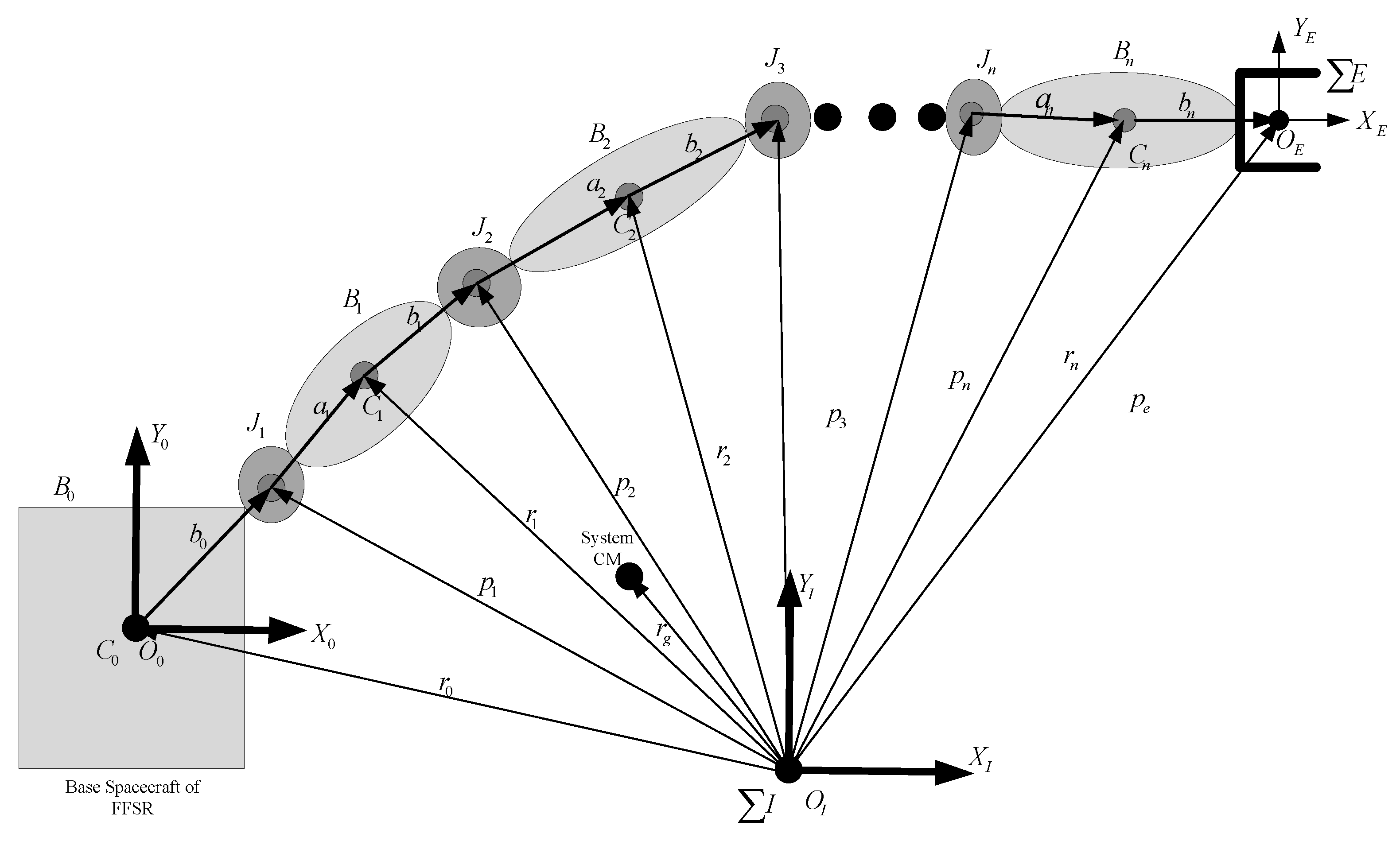
2.1. Kinematic Models of Space Robotic Systems
- (i= 0,...,n): mass center of body i;
- (i= 1,...,n): vector from joint i to mass center of body i with unit of [m; m; m], where m denotes the abbreviation of meter;
- (i= 0,...,n): vector from mass center of body i to joint with unit of [m; m; m];
- (i= 0,...,n): position of mass center of body i with unit of [m; m; m];
- (i= 1,...,n): position of joint i with unit of [m; m; m];
- : position of system centroid with unit of [m; m; m];
- : position of end effector with unit of [m; m; m];
- (i= 0,...,n): coordinate frame fixed on with origin and axes and ;
- : inertial coordinate frame with origin and axes and ; and
- : coordinate frame fixed on end effector with origin and axes and .
- : joint configuration with unit of each element of deg;
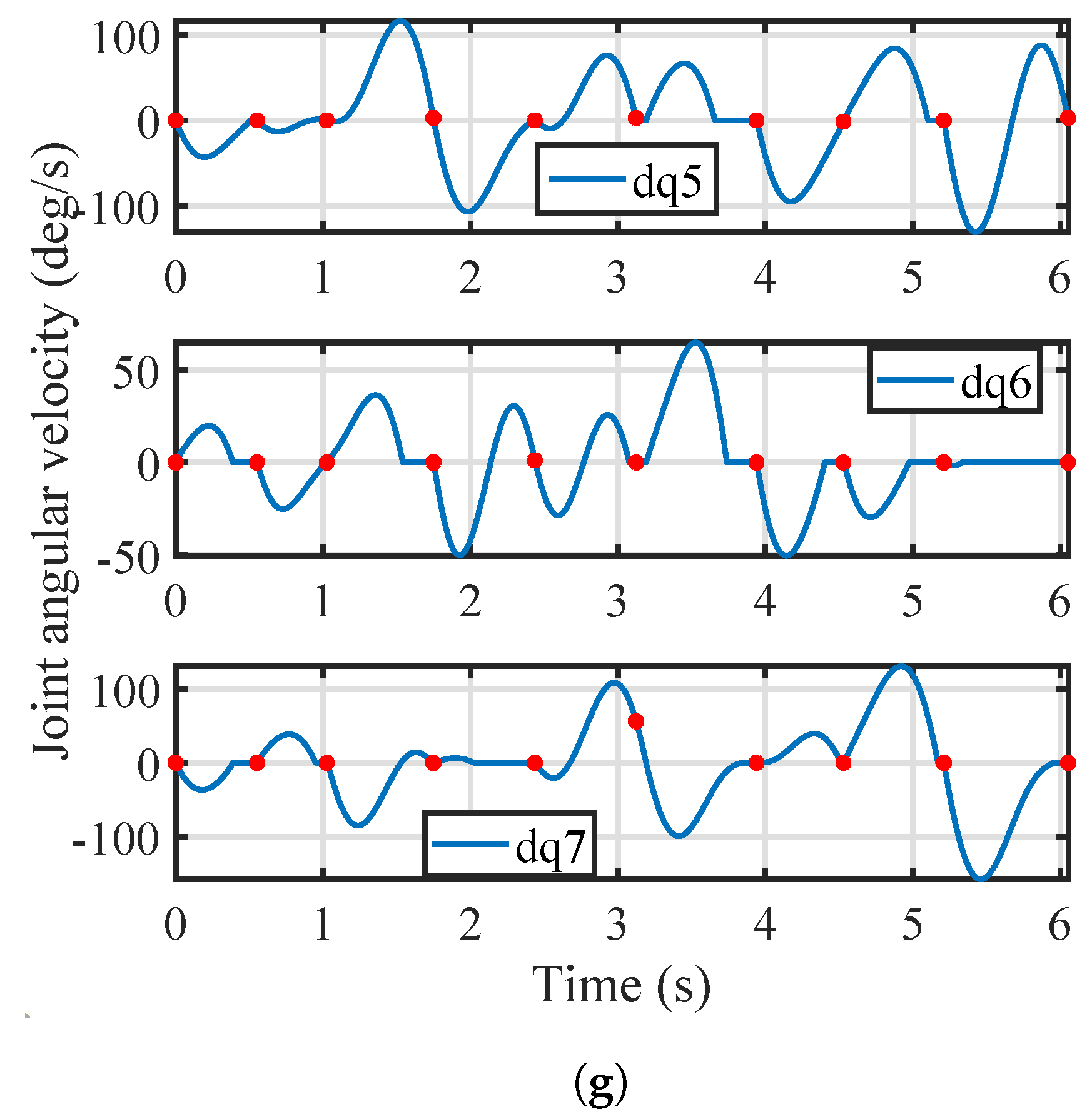
- : angular velocity of joint configuration with unit of each element of deg/s;
- : pose of base with unit of [m; m; m; deg; deg; deg];
- : velocity of base with unit of [m/s; m/s; m/s; deg/s; deg/s; deg/s];
- : linear velocity of end effector with unit of [m/s; m/s; m/s];
- : angular velocity of end effector with unit of [deg/s; deg/s; deg/s];
- : Jacobian matrix of base;
- : Jacobian matrix of manipulator;
- : coupling Jacobian matrix;
- : inertia matrix of base; and
- : coupling inertia matrix.
2.2. MTTP for Space Robotics
2.2.1. Objective Functions
A. Minimum Maneuver Time
B. Minimum Base Attitude Disturbance
2.2.2. Depiction of Joint Configurations Corresponding to Each Waypoint
- Step 1
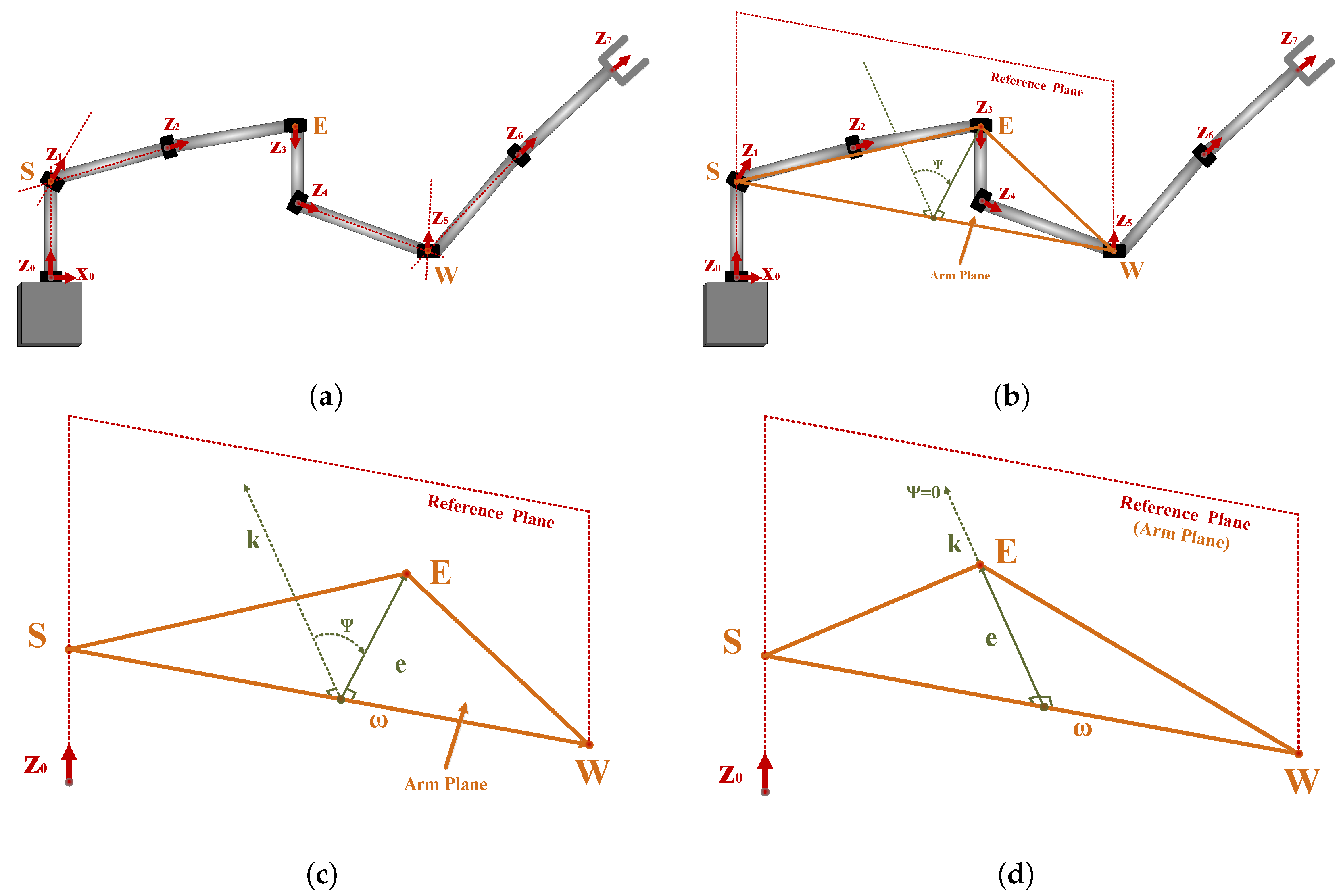
- Construction of the arm plane, the reference plane and the arm angle. First, the arm plane is constructed according to the points S, E, and W shown in Figure 2. Second, the reference plane is constructed based on and - or -axis, since at least one of - and -axes is not coincident with . The arm angle is then depicted, shown in Figure 2.
- Step 2
- Derivation of the joint angle . Project the arm plane to the plane perpendicular to the rotation axis of the elbow joint, namely -axis. According to the geometric construction of SRS and the Pythagorean theorem, two values of are derived.
- Step 3
- Derivation of the shoulder-joint angles , , and . First, the rotation transformation, rotating around with the rotation angle , is derived. Second, the orientation of relative to using the concept of the shoulder reference attitude matrix [32]. Finally, two groups of shoulder-joint angles are derived.
- Step 4
- Derivation of the wrist-joint angles , , and . Two groups of wrist-joint angles are derived according to the predefined attitude of the end effector, the rotation transformation and the should reference attitude matrix derived in Step 3, and the rotation matrix from to .
2.2.3. Formulation of Joint Trajectories among Waypoints
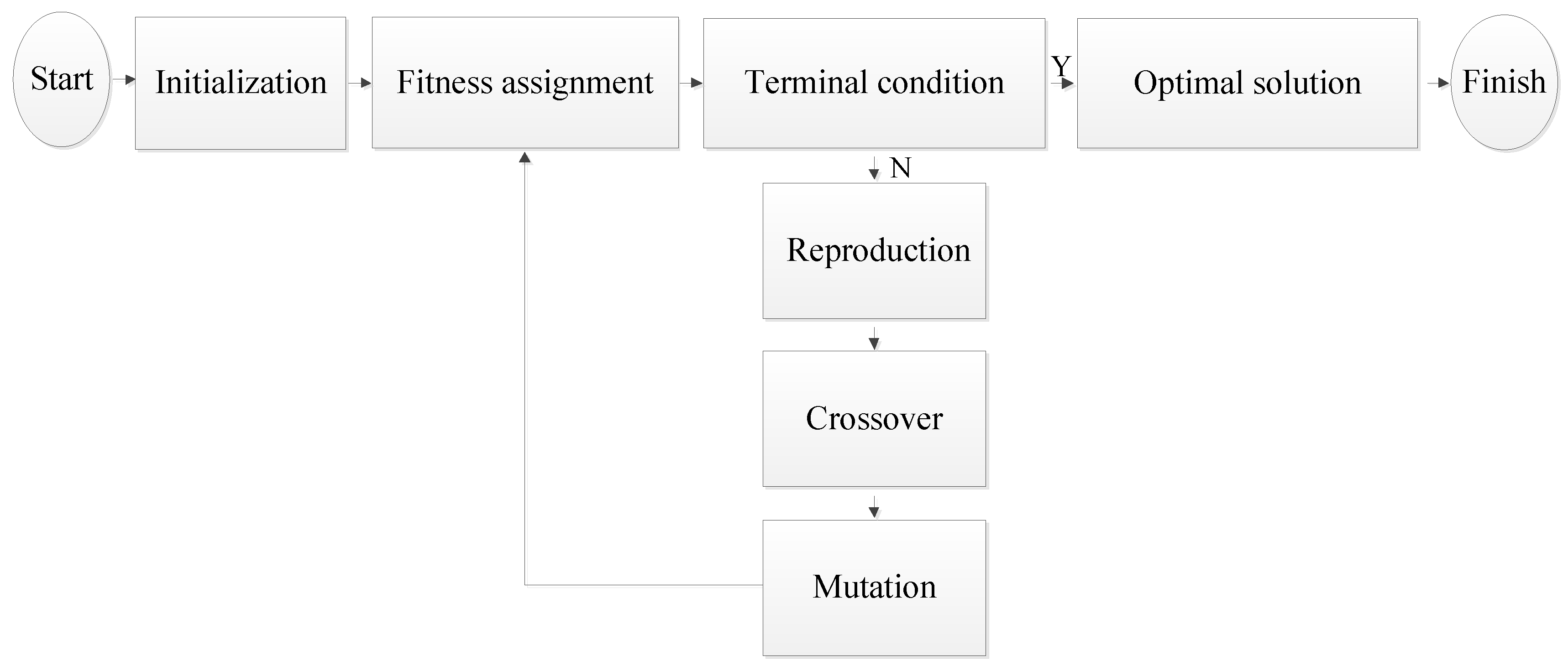
3. Improved Genetic Algorithm
3.1. Basic GA
3.2. Improved GA
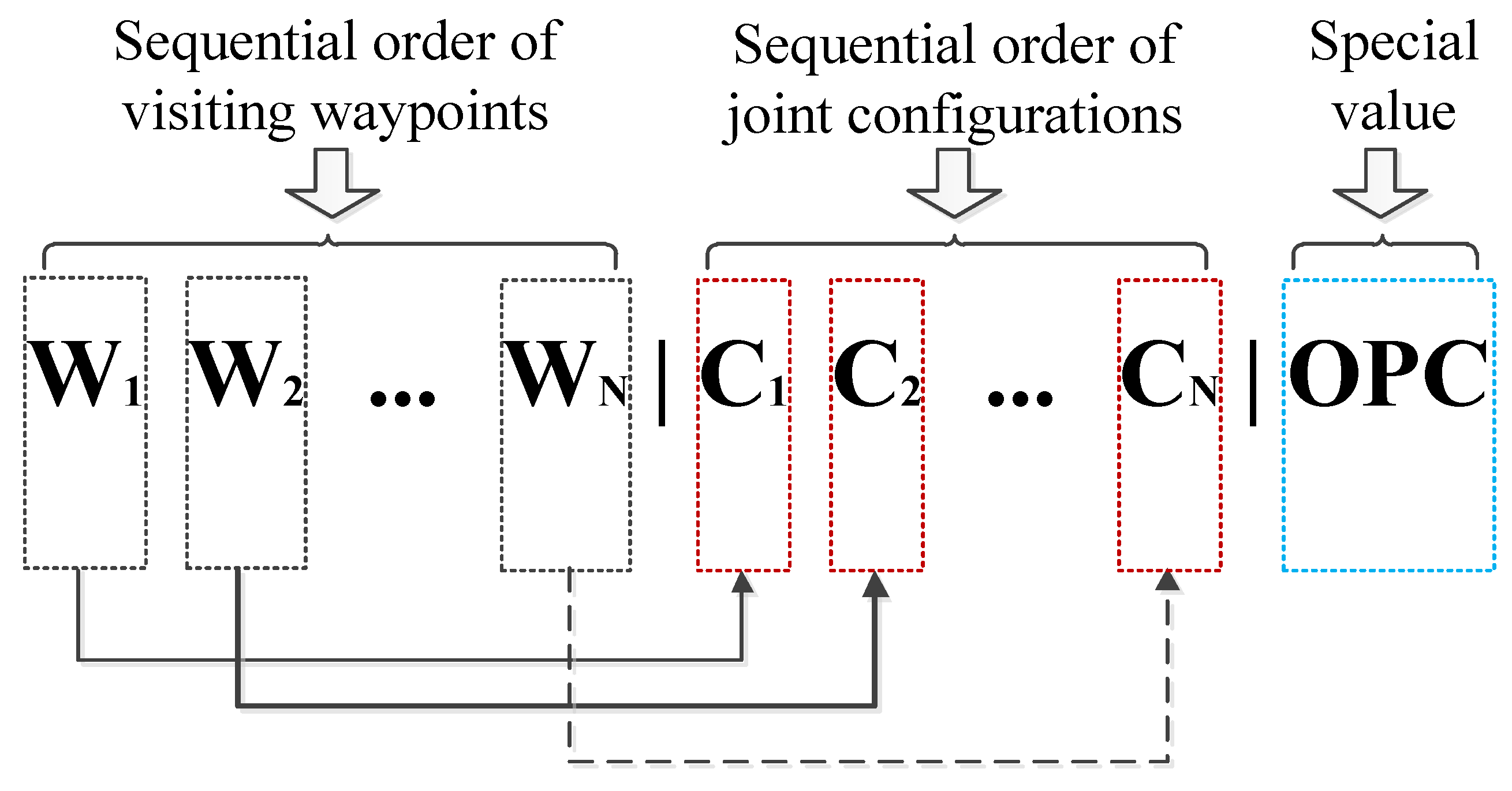
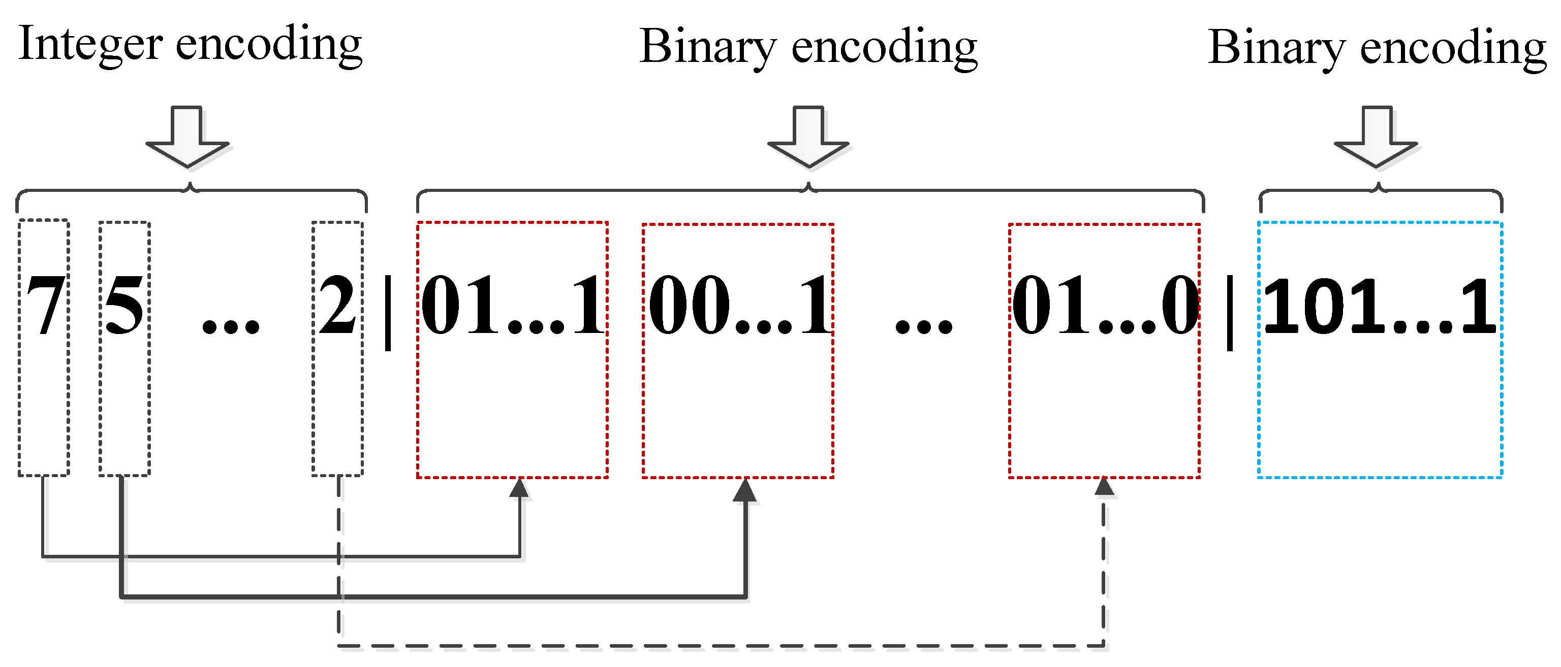
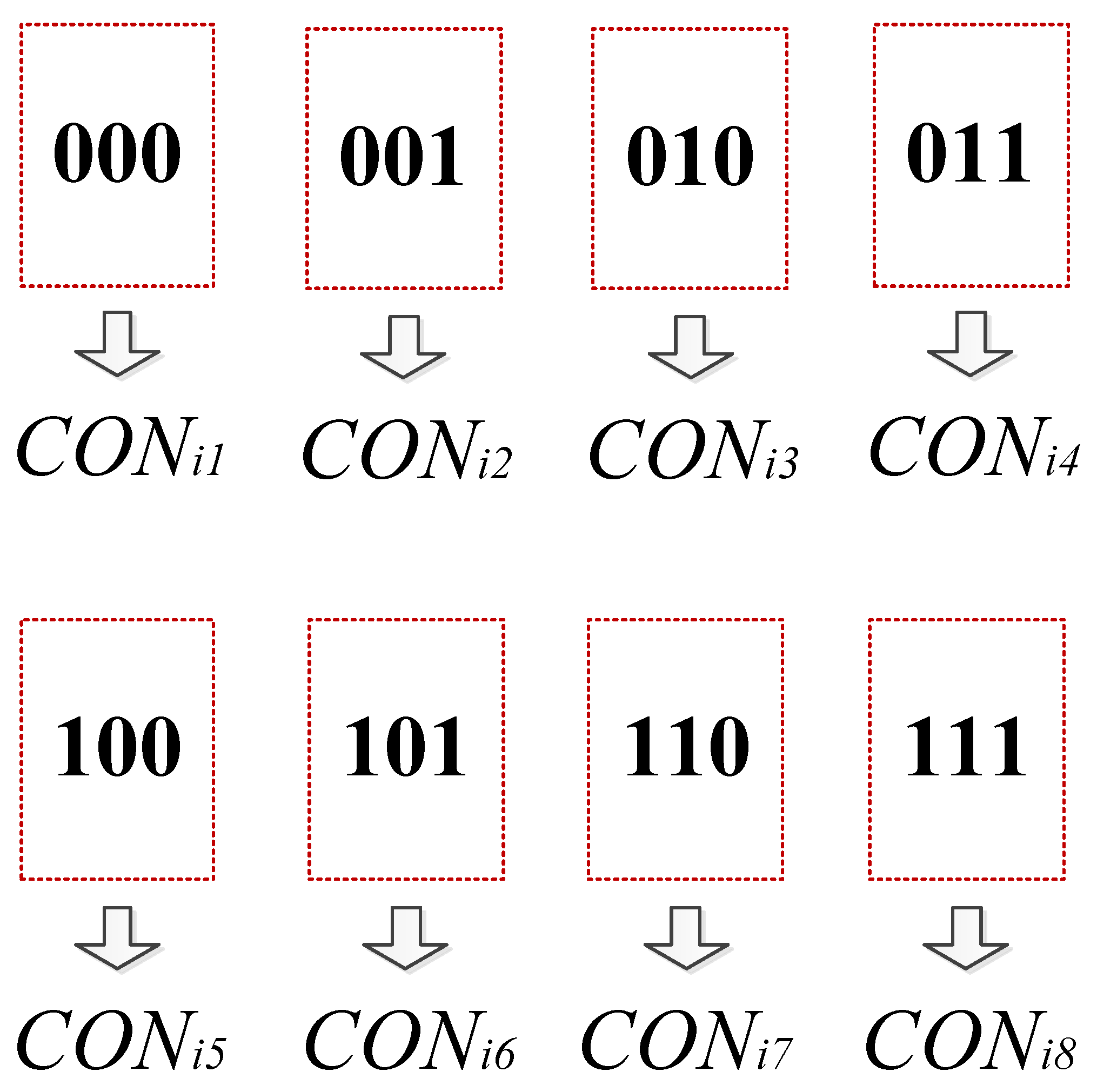
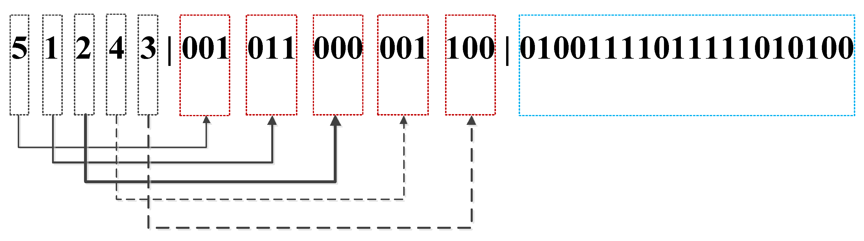
3.2.1. Encoding Mechanism
A. First Part of Each Chromosome
B. Second Part of Each Chromosome
C. Third Part of Each Chromosome
D. Example of Chromosome Depiction
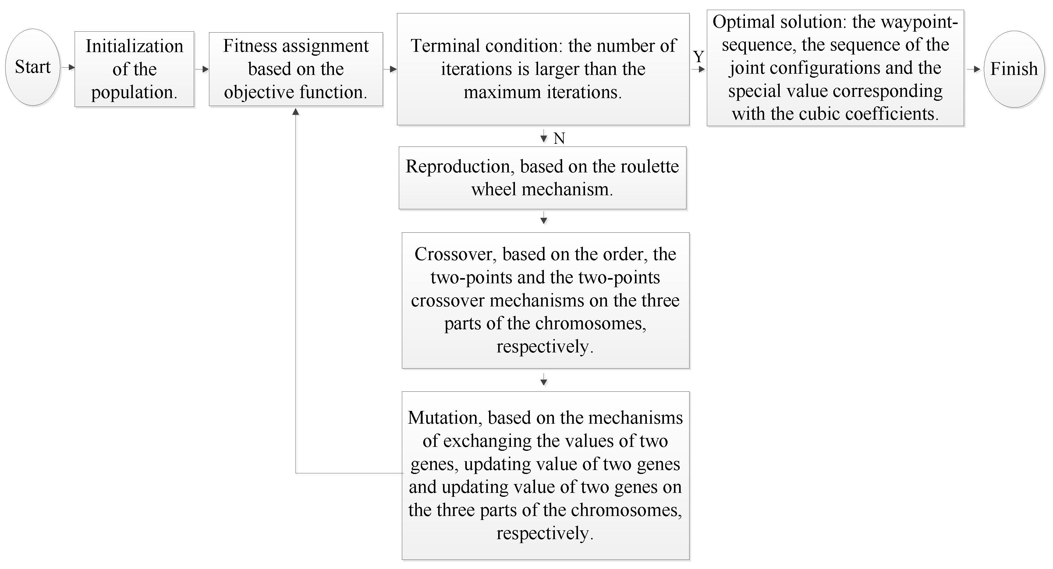
3.2.2. Updating Mechanism
A. Initialization
B. Reproduction
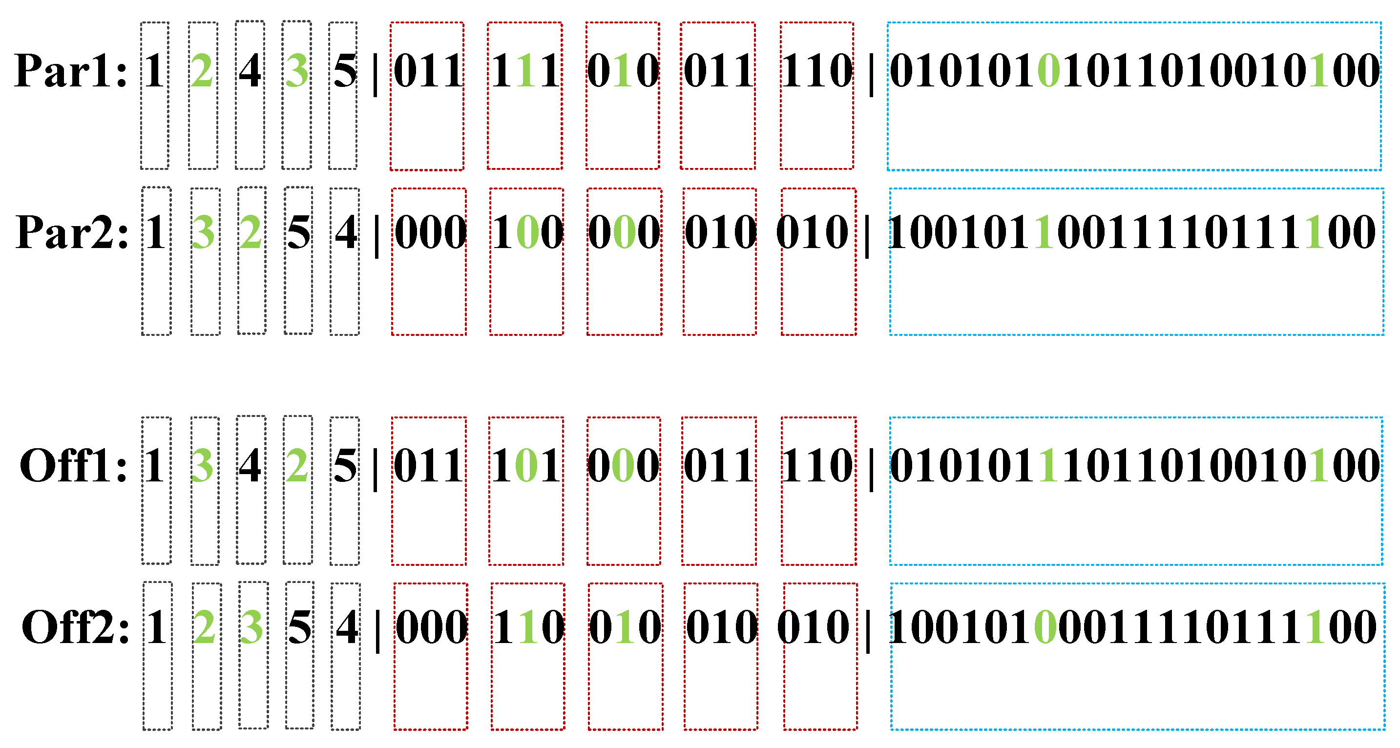
C. Crossover
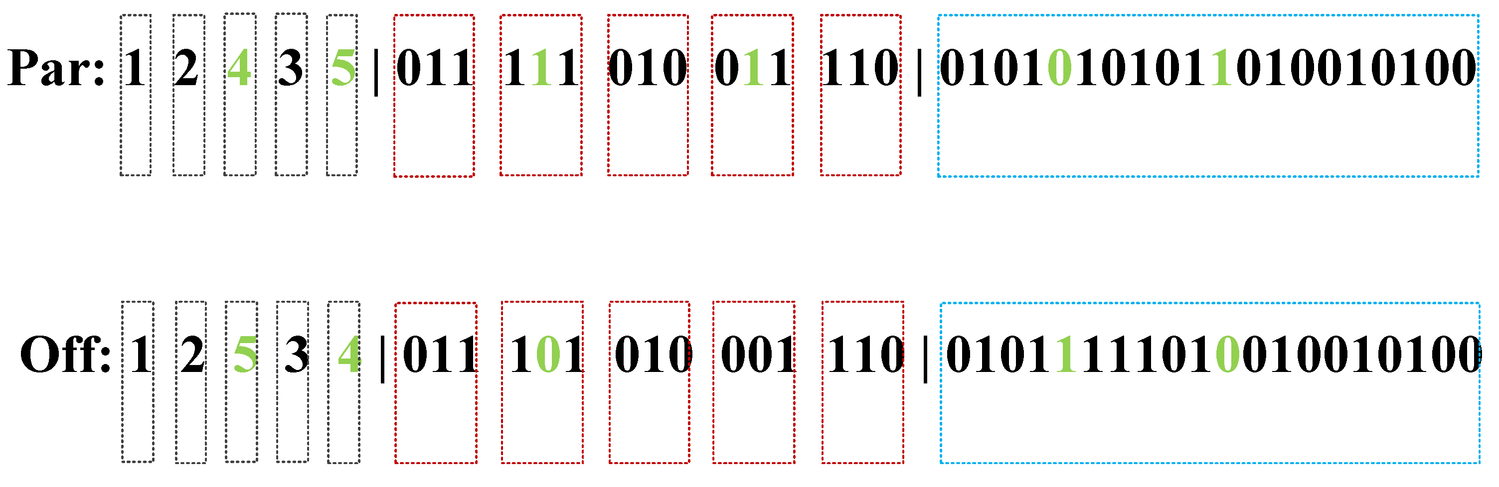
D. Mutation
3.2.3. IGA Work Mechanism
4. Numerical Simulations
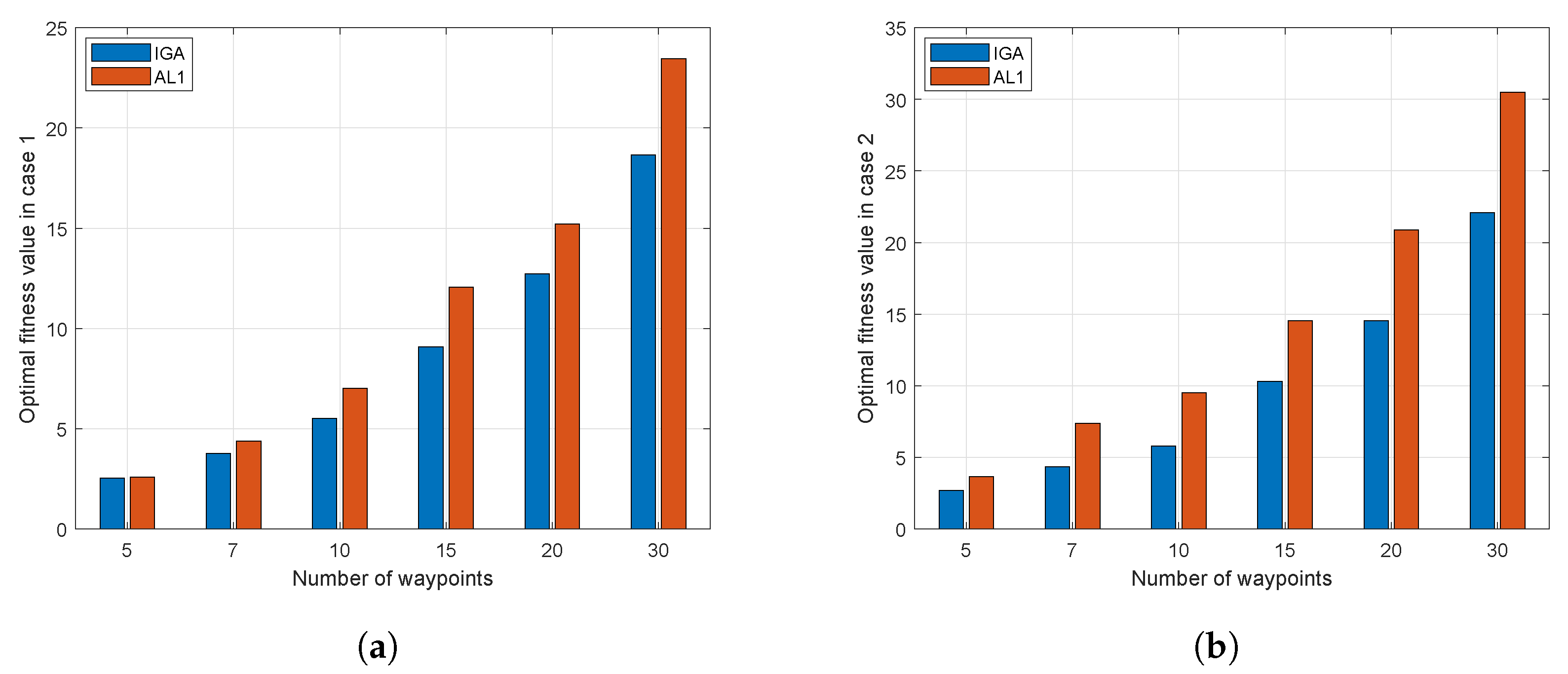
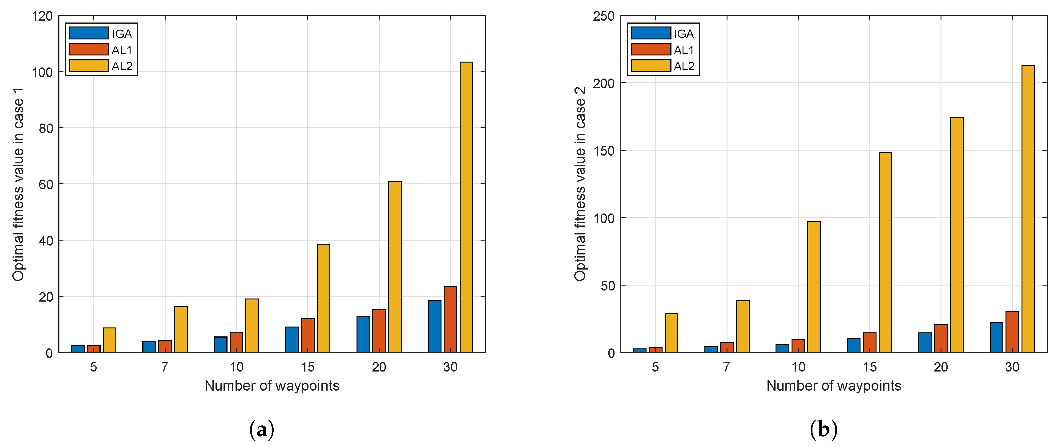
4.1. Comparisons
4.2. Simulation Cases
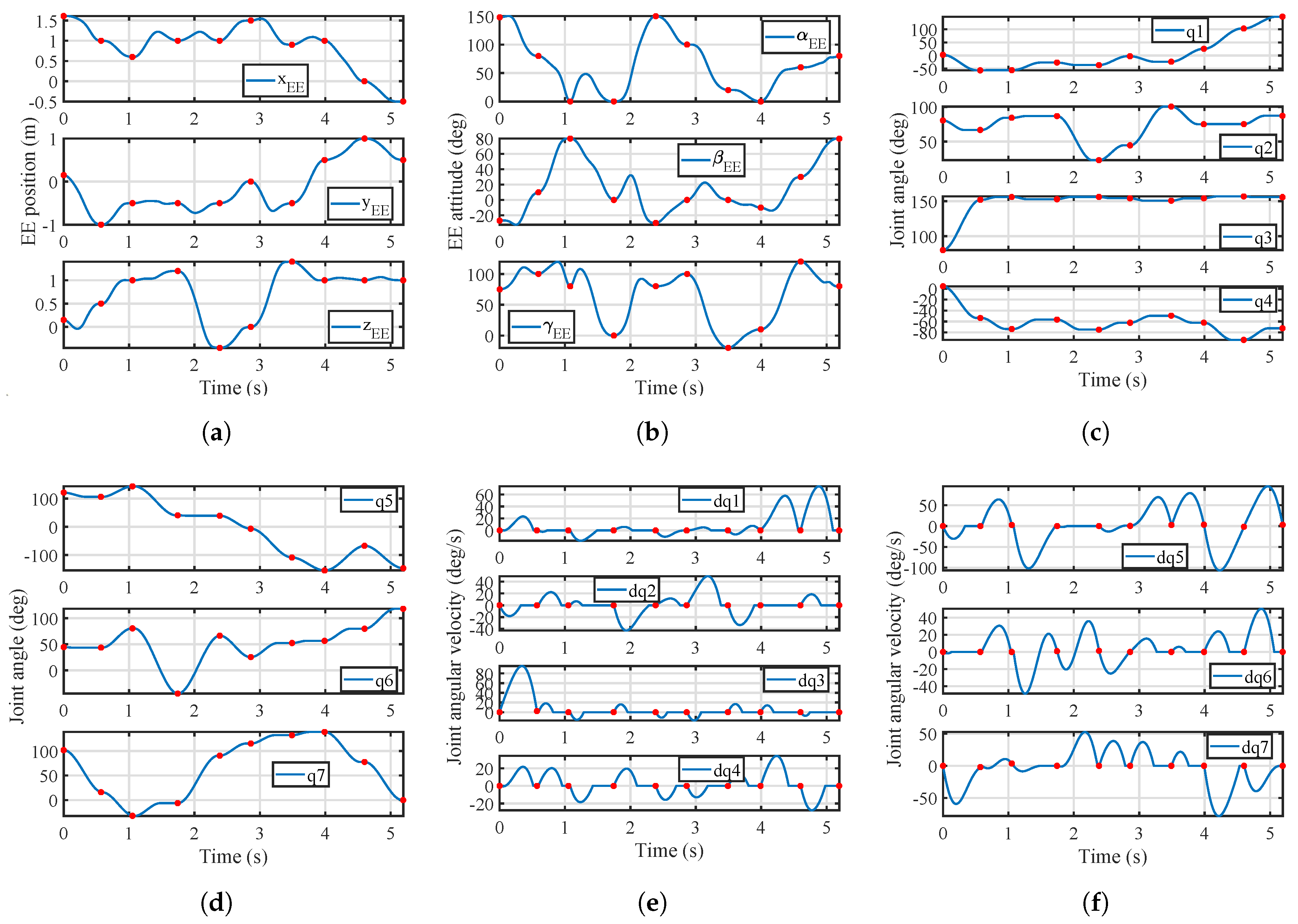
4.2.1. Case 1
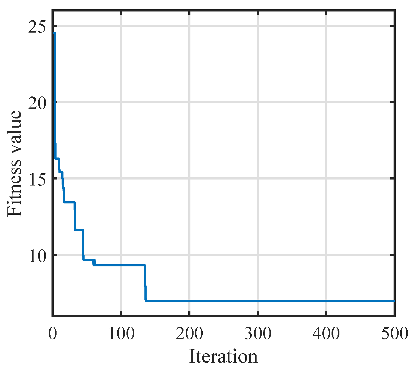
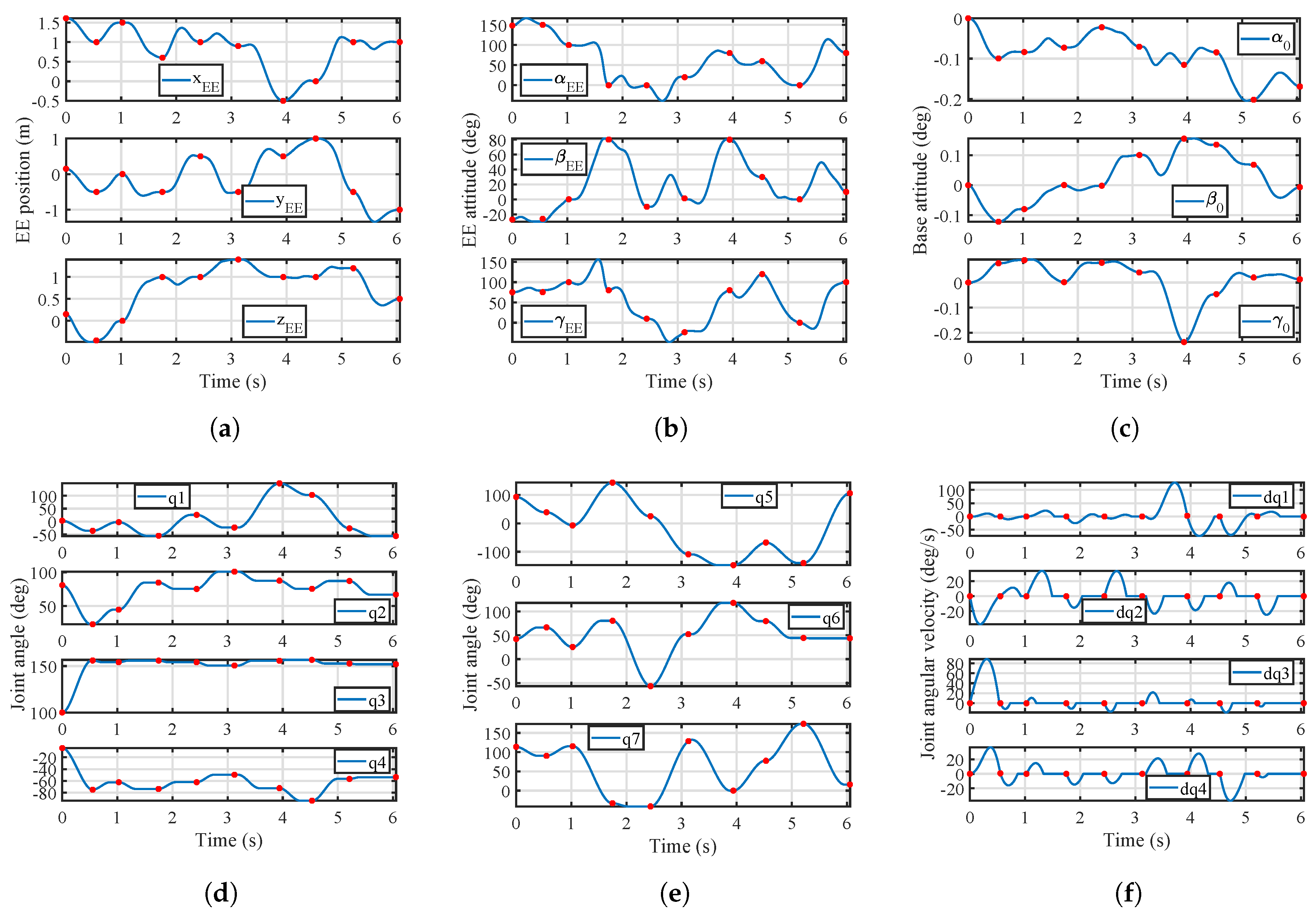
4.2.2. Case 2
5. Conclusions
- (i)
- Cubic coefficients of arguments of piecewise-sine functions share the same absolute value, making the third part of each chromosome only consider one value after decoding. Therefore, computational cost is reduced.
- (ii)
- In contrast to the setting on joint angular velocities in most recent studies about the MTTP for industrial robotics, each joint angular velocity varies based on Equation (10), contributing to the high-precision results.
Author Contributions
Funding
Acknowledgments
Conflicts of Interest
Abbreviations
| 2D | Two-dimensional |
| AET | Average execution time |
| AF | Average fitness |
| AL1 | Algorithm 1 |
| AL2 | Algorithm 2 |
| BF | Best fitness |
| D-H | Denavit-Hartenberg |
| DE | Differential evolution algorithm |
| DOF | Degree of freedom |
| EST-VII | Experimental Test Satellite VII |
| FFSR1 | Free-flying space robot |
| FFSR2 | Free-floating space robot |
| GA | Genetic algorithm |
| IGA | Improved genetic algorithm |
| ISS | International Space Station |
| JAXA | Japan Aerospace Exploration Agency |
| JEMRMS | Japanese Experiment Module Remote Manipulator System |
| MDA | MacDonald Dettwiler and Associates Ltd. |
| MTTP | Multitask-based trajectory-planning problem |
| PSO | Particle-swarm optimization algorithm |
| SRS | Spherical revolute spherical |
| TSP | Traveling salesman problem |
| WF | Worst fitness |
References
- Bowman, L.M.; Belvin, W.K.; Komendera, E.E.; Dorsey, J.T.; Doggett, B.R. In-space assembly application and technology for NASA’s future science observatory and platform missions. In Proceedings of the Space Telescopes and Instrumentation: Optical, Infrared, and Millimeter Wave, Austin, TX, USA, 10–15 June 2018. [Google Scholar] [CrossRef]
- Bonneville, R. A truly international lunar base as the next logical step for human spaceflight. Adv. Space Res. 2018, 61, 2983–2988. [Google Scholar] [CrossRef]
- Sato, N.; Doi, S. JEM remote manipulator system (JEMRMS) human-in-the-loop test. In Proceedings of the International Symposium on Space Technology and Science, Morioka, Japan, 28 May–4 June 2000. [Google Scholar]
- Rembala, R.; Ower, C. Robotic assembly and maintenance of future space stations based on the ISS mission operations experience. Acta Astronaut. 2009, 65, 912–920. [Google Scholar] [CrossRef]
- Oda, M.; Kibe, K.; Yamagata, F. ETS-VII, space robot in-orbit experiment satellite. In Proceedings of the IEEE International Conference on Robotics and Automation, Minneapolis, MN, USA, 22–28 April 1996; pp. 739–744. [Google Scholar] [CrossRef]
- Hirzinger, G.; Brunner, B.; Dietrich, J.; Heindl, J. ROTEX-the first remotely controlled robot in space. In Proceedings of the IEEE International Conference on Robotics and Automation, San Diego, CA, USA, 8–13 May 1994; pp. 2604–2611. [Google Scholar] [CrossRef]
- Umetani, Y.; Yoshida, K. Resolved motion rate control of space manipulators with generalized Jacobian matrix. IEEE Trans. Robot. Autom. 1989, 5, 303–314. [Google Scholar] [CrossRef]
- Dubowsky, S.; Torres, M.A. Path planning for space manipulators to minimize spacecraft attitude disturbances. In Proceedings of the IEEE International Conference on Robotics and Automation, Sacramento, CA, USA, 9–11 April 1991; pp. 2522–2528. [Google Scholar] [CrossRef]
- Papadopoulos, E.; Dubowsky, S. Dynamic singularities in free-floating space manipulators. In Space Robotics: Dynamics and Control; Xu, Y., Kanade, T., Eds.; Springer: Boston, MA, USA, 1993; pp. 77–100. ISBN 978-1-4615-3588-1. [Google Scholar]
- Yoshida, K.; Hashizume, K.; Abiko, S. Zero reaction maneuver: Flight validation with ETS-VII space robot and extension to kinematically redundant arm. In Proceedings of the IEEE International Conference on Robotics and Automation, Seoul, Korea, 21–26 May 2001; pp. 441–446. [Google Scholar] [CrossRef]
- Liu, X.; Baoyin, H.; Ma, X. Optimal path planning of redundant free-floating revolute-jointed space manipulators with seven links. Multibody Syst. Dyn. 2013, 29, 41–56. [Google Scholar] [CrossRef]
- Wang, M.; Luo, J.; Walter, U. Trajectory planning of free-floating space robot using Particle Swarm Optimization (PSO). Acta Astronaut. 2015, 112, 77–88. [Google Scholar] [CrossRef]
- Xu, W.; Li, C.; Liang, B.; Liu, Y.; Xu, Y. The Cartesian path planning of free-floating space robot using particle swarm optimization. Int. J. Adv. Robot Syst. 2008, 5, 301–310. [Google Scholar] [CrossRef]
- Xu, W.; Liu, Y.; Liang, B.; Xu, Y.; Li, C.; Qiang, W. Non-holonomic path planning of a free-floating space robotic system using genetic algorithms. Adv. Robot. 2008, 22, 451–476. [Google Scholar] [CrossRef]
- Chen, Z.; Zhou, W. Path planning for a space-based manipulator system based on quantum genetic algorithm. J. Robot. 2017, 2017. [Google Scholar] [CrossRef]
- Zhang, J.; Wei, X.; Zhou, D.; Zhang, Q. Trajectory planning of a redundant space manipulator based on improved hybrid PSO algorithm. In Proceedings of the IEEE International Conference on Robotics and Biomimetics (ROBIO), Qingdao, China, 3–7 December 2016; pp. 419–425. [Google Scholar] [CrossRef]
- Wang, M.; Luo, J.; Fang, J.; Yuan, J. Optimal trajectory planning of free-floating space manipulator using differential evolution algorithm. Adv. Space Res. 2018, 61, 1525–1536. [Google Scholar] [CrossRef]
- Alatartsev, S.; Stellmacher, S.; Ortmeier, F. Robotic task sequencing problem: A survey. J. Intell. Robot. Syst. 2015, 80, 279–298. [Google Scholar] [CrossRef]
- Bonami, P.; Olivares, A.; Staffetti, E. Energy-optimal multi-goal motion planning for planar robot manipulators. J. Optim. Theory Appl. 2014, 163, 80–104. [Google Scholar] [CrossRef]
- Little, J.D.; Murty, K.G.; Sweeney, D.W.; Karel, C. An algorithm for the traveling salesman problem. Oper. Res. 1963, 11, 972–989. [Google Scholar] [CrossRef]
- Gentilini, I.; Margot, F.; Shimada, K. The travelling salesman problem with neighbourhoods: MINLP solution. Optim. Method Softw. 2013, 28, 364–378. [Google Scholar] [CrossRef]
- Zacharia, P.T.; Aspragathos, N.A. Optimal robot task scheduling based on genetic algorithms. Robot. Cim-Int. Manuf. 2005, 21, 67–79. [Google Scholar] [CrossRef]
- Baizid, K.; Chellali, R.; Yousnadj, A.; Meddahi, A.; Bentaleb, T. Genetic algorithms based method for time optimization in robotized site. In Proceedings of the IEEE/RSJ International Conference on Intelligent Robots and Systems, Taipei, Taiwan, 18–22 October 2010; pp. 1359–1364. [Google Scholar] [CrossRef]
- Baizid, K.; Yousnadj, A.; Meddahi, A.; Chellali, R.; Iqbal, J. Time scheduling and optimization of industrial robotized tasks based on genetic algorithms. Robot. Cim-Int. Manuf. 2015, 34, 140–150. [Google Scholar] [CrossRef]
- Suárez-Ruiz, F.; Lembono, T.S.; Pham, Q.C. RoboTSP-a fast solution to the robotic task sequencing problem. In Proceedings of the IEEE International Conference on Robotics and Automation, Brisbane, Australia, 21–25 May 2018; pp. 1611–1616. [Google Scholar] [CrossRef]
- Bänziger, T.; Kunz, A.; Wegener, K. Optimizing human–robot task allocation using a simulation tool based on standardized work descriptions. J. Intell. Manuf. 2018, 1–14. [Google Scholar] [CrossRef]
- Kovács, A. Task sequencing for remote laser welding in the automotive industry. In Proceedings of the Twenty-Third International Conference on Automated Planning and Scheduling, Rome, Italy, 10–14 June 2013; pp. 457–461. [Google Scholar]
- Saha, M.; Roughgarden, T.; Latombe, J.C.; Sánchez-Ante, G. Planning tours of robotic arms among partitioned goals. Int. J. Robot. Res. 2006, 25, 207–223. [Google Scholar] [CrossRef]
- Gbenga, D.E.; Ramlan, E.I. Understanding the limitations of particle swarm algorithm for dynamic optimization tasks: A survey towards the singularity of PSO for swarm robotic applications. ACM Comput. Surv. 2016, 49. [Google Scholar] [CrossRef]
- Li, G.; Zhang, F.; Fu, Y.; Wang, S. Joint stiffness identification and deformation compensation of serial robots based on dual quaternion algebra. Appl. Sci. 2019, 9, 65. [Google Scholar] [CrossRef]
- Xue, Y. Mobile robot path planning with a non-dominated sorting genetic algorithm. Appl. Sci. 2018, 8, 2253. [Google Scholar] [CrossRef]
- Xu, W.; Yan, L.; Mu, Z.; Wang, Z. Dual arm-angle parameterisation and its applications for analytical inverse kinematics of redundant manipulators. Robotica 2016, 34, 2669–2688. [Google Scholar] [CrossRef]
- Waldron, K.; Schmiedeler, J. Kinematics. In Springer Handbook of Robotics; Siciliano, B., Khatib, O., Eds.; Springer: Berlin, Germany, 2016; pp. 11–36. ISBN 978-3-319-32550-7. [Google Scholar]
- Siciliano, B.; Sciavicco, L.; Villani, L.; Oriolo, G. Robotics: Modelling, Planning and Control; Springer: London, UK, 2010; pp. 39–104. ISBN 978-1-84628-641-4. [Google Scholar]
- Zhou, D.; Ji, L.; Zhang, Q.; Wei, X. Practical analytical inverse kinematic approach for 7-DOF space manipulators with joint and attitude limits. Intel. Serv. Robot. 2015, 8, 215–224. [Google Scholar] [CrossRef]
- Shimizu, M.; Kakuya, H.; Yoon, W.K.; Kitagaki, K.; Kosuge, K. Analytical inverse kinematic computation for 7-DOF redundant manipulators with joint limits and its application to redundancy resolution. IEEE Trans. Robot. 2008, 24, 1131–1142. [Google Scholar] [CrossRef]
- Yu, C.; Jin, M.; Liu, H. An analytical solution for inverse kinematic of 7-DOF redundant manipulators with offset-wrist. In Proceedings of the IEEE International Conference on Mechatronics and Automation, Chengdu, China, 5–8 August 2012; pp. 92–97. [Google Scholar] [CrossRef]
- Holland, J.H. Adaptation in Natural and Artificial Systems Ann Arbor; University of Michigan Press: Ann Arbor, MI, USA, 1975. [Google Scholar]
- Goldberg, D.E. Genetic Algorithm in Search, Optimization and Machine Learning; Addison Wesley: Boston, MA, USA, 1989. [Google Scholar]
- Grefenstette, J.; Gopal, R.; Rosmaita, B.; Van Gucht, D. Genetic algorithms for the traveling salesman problem. In Proceedings of the First International Conference on Genetic Algorithms and their Applications, Pittsburgh, PA, USA, 24–26 July 1985; pp. 160–168. [Google Scholar]
- Abed, I.A.; Koh, S.P.; Sahari, K.S.M.; Tiong, S.K.; Tan, N.M. Optimization of task scheduling for single-robot manipulator using pendulum-like with attraction-repulsion mechanism algorithm and genetic algorithm. Aust. J. Basic Appl. Sci. 2013, 7, 426–445. [Google Scholar]


| Body | Mass | Length | Principle Moment of Inertial (kg ) | ||
|---|---|---|---|---|---|
| (kg) | (m) | ||||
| 0 | 500 | 100 | 100 | 200 | |
| 1 | 20 | 4 | 4 | 5 | |
| 2 | 10 | 2 | 2 | 3 | |
| 3 | 50 | 10 | 10 | 20 | |
| 4 | 20 | 4 | 4 | 5 | |
| 5 | 50 | 10 | 10 | 20 | |
| 6 | 10 | 2 | 2 | 3 | |
| 7 | 20 | 4 | 4 | 5 | |
| No. | C1AET | C1WF | C1BF | C1AF | C2AET | C2WF | C2BF | C2AF |
|---|---|---|---|---|---|---|---|---|
| 5 | ||||||||
| 7 | ||||||||
| 10 | ||||||||
| 15 | ||||||||
| 20 | ||||||||
| 30 |
| No. | C1AET | C1WF | C1BF | C1AF | C2AET | C2WF | C2BF | C2AF |
|---|---|---|---|---|---|---|---|---|
| 5 | ||||||||
| 7 | ||||||||
| 10 | ||||||||
| 15 | ||||||||
| 20 | ||||||||
| 30 |
| No. | C1AET | C1WF | C1BF | C1AF | C2AET | C2WF | C2BF | C2AF |
|---|---|---|---|---|---|---|---|---|
| 5 | ||||||||
| 7 | ||||||||
| 10 | ||||||||
| 15 | ||||||||
| 20 | ||||||||
| 30 |
| No. | Position (m) | Attitude (deg) |
|---|---|---|
| 1 | ||
| 2 | ||
| 3 | ||
| 4 | ||
| 5 | ||
| 6 | ||
| 7 | ||
| 8 | ||
| 9 | ||
| 10 |
© 2019 by the authors. Licensee MDPI, Basel, Switzerland. This article is an open access article distributed under the terms and conditions of the Creative Commons Attribution (CC BY) license (http://creativecommons.org/licenses/by/4.0/).
Share and Cite
Zhao, S.; Zhu, Z.; Luo, J. Multitask-Based Trajectory Planning for Redundant Space Robotics Using Improved Genetic Algorithm. Appl. Sci. 2019, 9, 2226. https://doi.org/10.3390/app9112226
Zhao S, Zhu Z, Luo J. Multitask-Based Trajectory Planning for Redundant Space Robotics Using Improved Genetic Algorithm. Applied Sciences. 2019; 9(11):2226. https://doi.org/10.3390/app9112226
Chicago/Turabian StyleZhao, Suping, Zhanxia Zhu, and Jianjun Luo. 2019. "Multitask-Based Trajectory Planning for Redundant Space Robotics Using Improved Genetic Algorithm" Applied Sciences 9, no. 11: 2226. https://doi.org/10.3390/app9112226
APA StyleZhao, S., Zhu, Z., & Luo, J. (2019). Multitask-Based Trajectory Planning for Redundant Space Robotics Using Improved Genetic Algorithm. Applied Sciences, 9(11), 2226. https://doi.org/10.3390/app9112226