An Optical Interference Suppression Scheme for TCSPC Flash LiDAR Imagers

Featured Application

This work is relevant in the context of multi-user LiDAR applications where multiple LiDARs may be active in the same environment simultaneously. Automotive safety, driving assistance, robotic navigation, and automated industrial vehicles are a few examples of scenarios where interference among concurrent LiDARs quickly becomes a critical issue. In those applications, being able to guarantee interference-free LiDAR operation is a necessary step towards the realization of safe and reliable functions.

Abstract

This paper describes an optical interference suppression scheme that allows flash light detection and ranging (LiDAR) imagers to run safely and reliably in uncontrolled environments where multiple LiDARs are expected to operate concurrently. The issue of optical interference is a potential show-stopper for the adoption of flash LiDAR as a technology of choice in multi-user application fields such as automotive sensing and autonomous vehicle navigation. The relatively large emission angle and field of view of flash LiDAR imagers make them especially vulnerable to optical interference. This work illustrates how a time-correlated single-photon counting LiDAR can control the timing of its laser emission to reduce its statistical correlation to other modulated or pulsed light sources. This method is based on a variable random delay applied to the laser pulse generated by LiDAR and to the internal circuitry measuring the time-of-flight. The statistical properties of the pseudorandom sequence of delays determines the effectiveness of LiDAR resilience against unintentional and intentional optical interference. For basic multi-camera operation, a linear feedback shift register (LFSR) was used as a random delay generator, and the performance of the interference suppression was evaluated as a function of sequence length and integration time. Direct interference from an identical LiDAR emitter pointed at the same object was reduced up to 50 dB. Changing integration time between 10 ms and 100 ms showed a marginal impact on the performance of the suppression (less than 3 dB deviation). LiDAR signal integrity was characterized during suppression, obtaining a maximum relative deviation of the measured time-of-flight of 0.1%, and a maximum deviation of measurements spread (full-width half-maximum) of 3%. The LiDAR signal presented an expected worst-case reduction in intensity of 25%.

1. Introduction

Light detection and ranging (LiDAR) is rapidly emerging as a key technology in automotive sensing, both for advanced driver assistance systems (ADAS) and as an enabler of fully autonomous driving [1]. The use of LiDAR as a complement to existing technologies, such as radar, ultrasonic range finding, thermal imaging, and image processing, is rapidly changing the landscape of advanced automotive sensor systems. The joint use of heterogeneous sensors, known as sensor fusion, promises to facilitate the safe implementation of level 3 and level 4 autonomy [2,3,4], and to be an enabling factor of fully autonomous driving [5]. Even outside the automotive field, where the reliable and safe navigation of autonomous or semi-autonomous machines is needed (e.g., advanced robotics, automated guided vehicles, factory automation, simultaneous localization and mapping, and drones), LiDAR is proving itself to be a valid complement to existing navigation sensors [6,7].

It is expected that the use of LiDAR in navigation applications will rise steadily in the future [1]. The widespread adoption of LiDAR in uncontrolled, multi-user environments will soon bring the problem of mutual optical interference to the fore. This paper describes an interference suppression scheme specifically designed for flash LiDAR cameras operating in time-correlated single-photon counting (TCSPC) mode, but the same principles are applicable to a wide variety of pulsed LiDAR techniques. The suppression scheme, referred to as FLISS (Flash LiDAR Interference Suppression Scheme) in the remainder of this paper, allows a TCSPC flash LiDAR to operate in an environment shared with other LiDARs without suffering from optical interference. FLISS does not require any form of coordination between cameras and can in principle reject optical interference generated by any type of device.

The paper will first present an overview of existing techniques for LiDAR interference management and relevant literature on the topic. A more formal description of interference in the context of flash LiDAR imagers will then be provided, followed by a presentation of the FLISS method. The paper will conclude with a section on experimental results and future directions.

2. TCSPC LiDAR

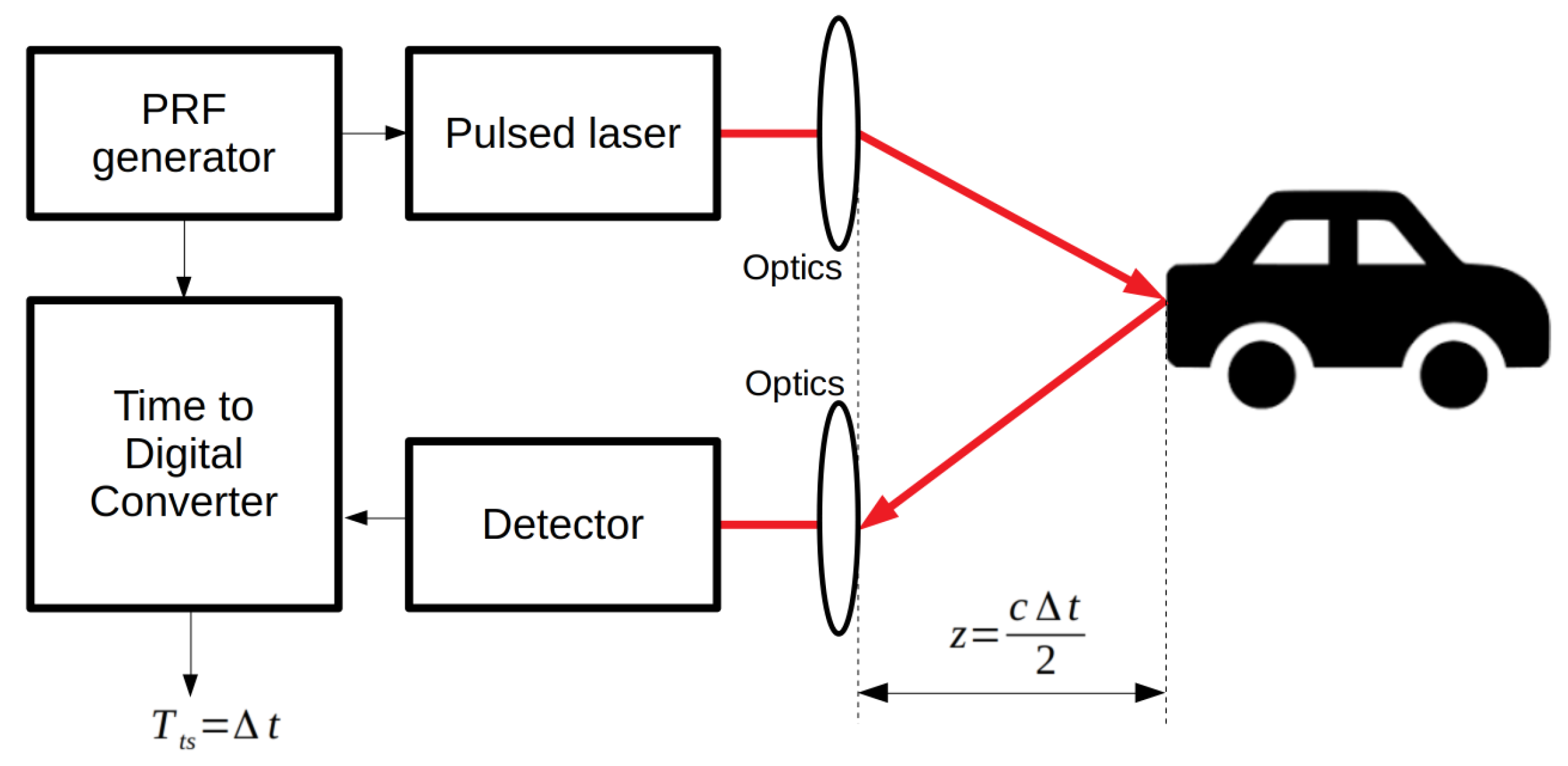
A TCSPC LiDAR is a type of direct time-of-flight (d-ToF) sensor. In direct time-of-flight (d-ToF), the distance z to an object is estimated by measuring the round trip time $T_{ToF}$ of an electromagnetic pulse (usually infrared light) from a suitable emitter contiguous to the detector to the object, according to the d-ToF relation

$$z=\frac{c·T_{ToF}}{2},$$

(1)

where c is the travel speed of the chosen electromagnetic wave in the propagation medium (Figure 1).

In optical TCSPC imaging (especially 3D range finding) emitters are usually chosen among Q-switched lasers [8] or vertical-cavity surface-emitting laser (VCSEL) arrays [9], due to their fast switching speeds.

Single-photon detectors such as single-photon avalanche diodes (SPADs) are used on the receiver side to detect the time of arrival of individual photons. Photoelectrons generated by the absorption of individual photons are accelerated by the strong electric field in the diode and undergo an avalanche multiplication process that produces a macroscopic, measurable current through the device [10]. Events detected by the SPAD pixels are often timed on-chip using combinations of time-to-analog converters (TACs) and analog-to-digital converters (ADCs) [11,12], or time-to-digital converters (TDCs) [13,14,15], to produce a digital representation of the time of arrival of each detected photon, called a timestamp. Each timestamp $T_{\mathrm{ts}}$ is a measure of the time of arrival of a photon detected by the pixel $T_{\mathrm{pixel}}$ relative to the generation time of the laser pulse $T_0$, according to the relation

$$T_{\mathrm{ts}}=T_{\mathrm{pixel}}-T_0=T_{ToF}-T_0.$$

(2)

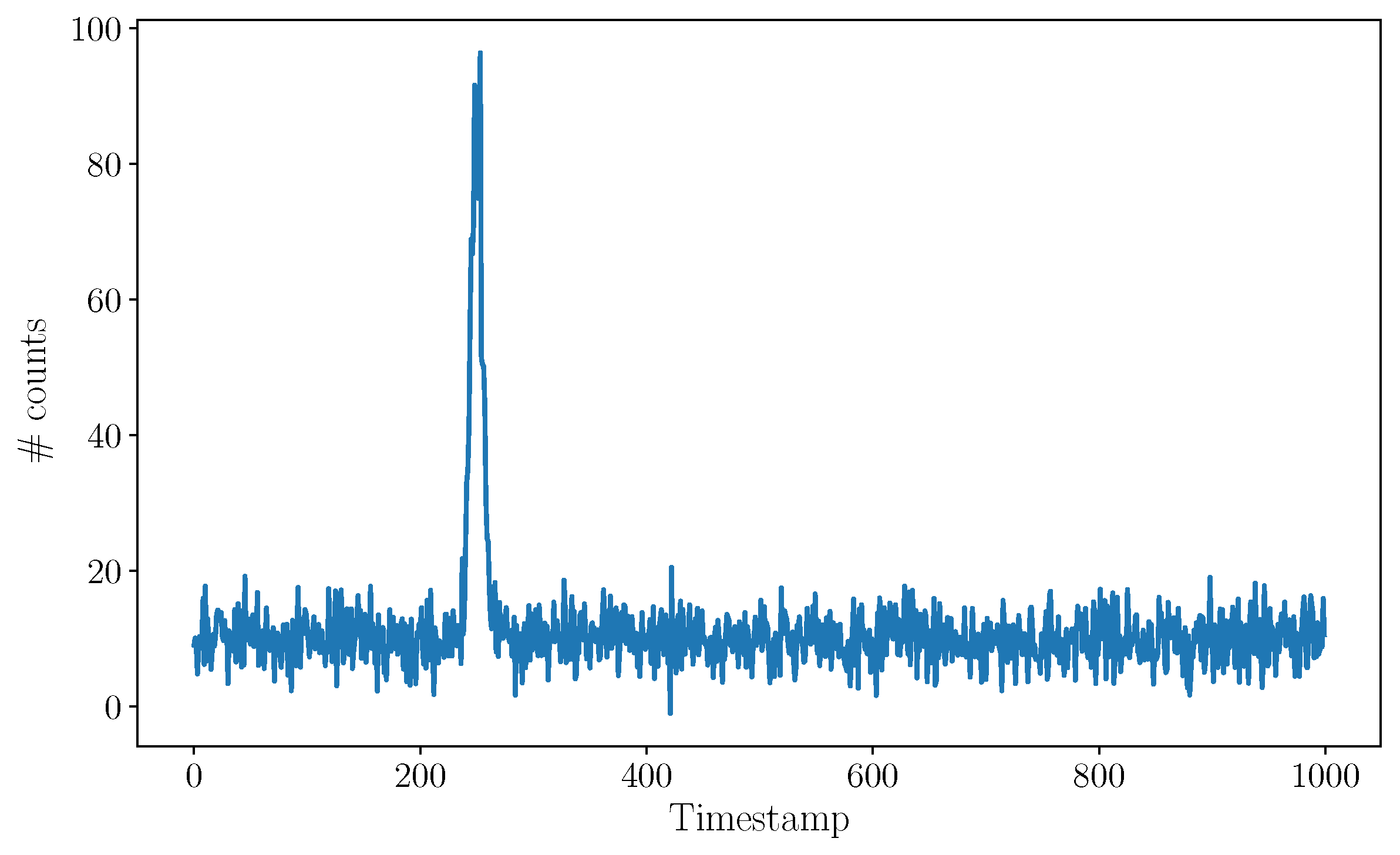
Given it is impossible to discriminate between the possible origins of each individual event produced by a SPAD pixel (thermal noise, ambient light, and active signal being the most prominent sources), TCSPC LiDAR imagers often repeat the same timestamp measurement 10–10,000 times. All measured timestamps undergo simple statistical processing to extract the relevant features of the useful signal. Ambient photon detections and dark counts (including thermally induced events and trap-assisted tunneling) occur at random times and are not correlated to the active signal. Active signal photons, on the other hand, are emitted synchronously to the activation instant of the TDC, and therefore, their time of arrival at the sensor is correlated and dependent on their time-of-flight (ToF). If plotted in a histogram, all detected timestamps will produce a noisy plateau representing uncorrelated events (ambient light and internal detector noise) and a peak constituted by the time of arrival of signal photons. A typical TCSPC histogram is shown in Figure 2.

3. Related Work

Several contributions have been published on topics that are closely related to LiDAR optical interference suppression. It is challenging, however, to pinpoint one main line of research on the topic, due to the variety of technologies and techniques available for 3D imaging and range finding.

Signal-to-noise ratio (SNR) improvement is often seen as a necessary step towards proper rejection of extraneous interference. Matched filter approaches [16] and customized digital post-processors [17] have been proposed to achieve high SNR of the LiDAR signal in avalanche photo-diode (APD)-based sensors.

One special case of LiDAR interference that has been studied extensively is the multi-path interference (MPI) [18,19,20,21], which is a LiDAR system interfering with itself through a plurality of optical paths, either as a consequence of the complex geometry of the imaged scene or the presence of semi-transparent or specular objects. Published approaches to MPI suppression include the use of multiple modulation frequencies in indirect time-of-flight (i-ToF) [22], sometimes in conjunction with compressive sensing to reconstruct multi-path reflections [23].

Proper multi-camera interference occurs when multiple LiDAR sensors operate in the same environment. Several techniques borrowed from telecommunications technology and signal processing theory are known to minimize the interference between multiple LiDAR cameras sharing the same communication channel: space-division multiple access (SDMA), frequency-division multiple access (FDMA), wavelength-division multiple access (WDMA), time-division multiple access (TDMA), and code-division multiple access (CDMA).

The SDMA method requires spatial separation of the LiDAR cameras so that their fields of view do not overlap. Each camera monitors a well-defined portion of space, and its emission never overlaps with the field of view of any other camera in the same environment. SDMA is scalable to an arbitrary number of cameras but is unsuitable for use in uncontrolled environments without considerable coordination between all the cameras.

In FDMA, each LiDAR camera must be assigned a unique operating frequency, which is represented by the pulse repetition frequency (PRF) in d-ToF. When operating at different PRFs, two LiDAR systems will not interfere with one another and will appear to each other as uncorrelated noise. The LiDAR PRFs must be separated enough to guarantee the minimization of systematic errors at short integration times, thereby limiting the maximum number of parallel channels. It should be noted that LiDAR imagers based on FDMA require coordination in uncontrolled environments in order to reassign the PRFs in the case of collision.

A popular option for optical devices such as LiDAR imagers is WDMA. WDMA mandates the use of multiple, non-overlapping optical channels centered on different wavelengths, separated on the receiver side by means of appropriate narrow-band optical filters. Such systems must handle the relatively low number of available channels in the operating band, which is limited by eye safety limits in the visible range, the bandwidth of the optical filter, the spectral purity of the emitter, and by the spectral sensitivity of the detector.

In TDMA, concurrent imagers are assigned unique, non-overlapping time intervals in which they are allowed to emit. TDMA side-steps the issue of interference by guaranteeing that at most one camera is active at any given time. The trade-off is of course the need to centrally coordinate all cameras (although peer-to-peer approaches are also possible).

The CDMA technique achieves interference suppression by borrowing alternative modulation schemes from spread-spectrum telecommunication systems. The basic idea of CDMA for LiDAR is that the light signal produced by each camera is shaped according to a specific digital or analog modulation scheme that allows the emitter to recognize its own signal over noise and interference. Detection and recognition are often performed by correlating the measured (noisy) signal with a specific correlation target function. The use of pseudorandom noise in i-ToF [24] falls into this broad category, as do phase-shift keying (PSK) modulation in TCSPC LiDARs [25] and the use of optical orthogonal codes [26,27].

Related research has been published on the topic of the identification and authentication of a LiDAR signal as one’s own by means of side-channel fingerprinting and advanced encryption standard (AES) encryption [28]. While unsuitable for solving the multi-camera interference problem per se, these techniques are important steps towards comprehensive security of the LiDAR channel.

4. LiDAR Optical Interference

This section provides some required definitions and a description of optical interference in the case of TCSPC LiDAR imagers.

In the context of this paper, a victim is a TCSPC LiDAR system potentially subject to optical interference. We define optical interference as any optical signal possessing the following properties.

• The signal is modulated or pulsed, so as to appear distinctly different in its temporal evolution from ambient light or detector noise in the victim.
• The signal is actively generated by a third party, potentially a TCSPC LiDAR of the same nature as the victim.
• The signal is detected by the victim.

The saturation of the detector is not considered as optical interference. Issues related to pile-up distortion and saturation, including strong sunlight and the intentional blinding of the victim, remain open and should be addressed by different methods.

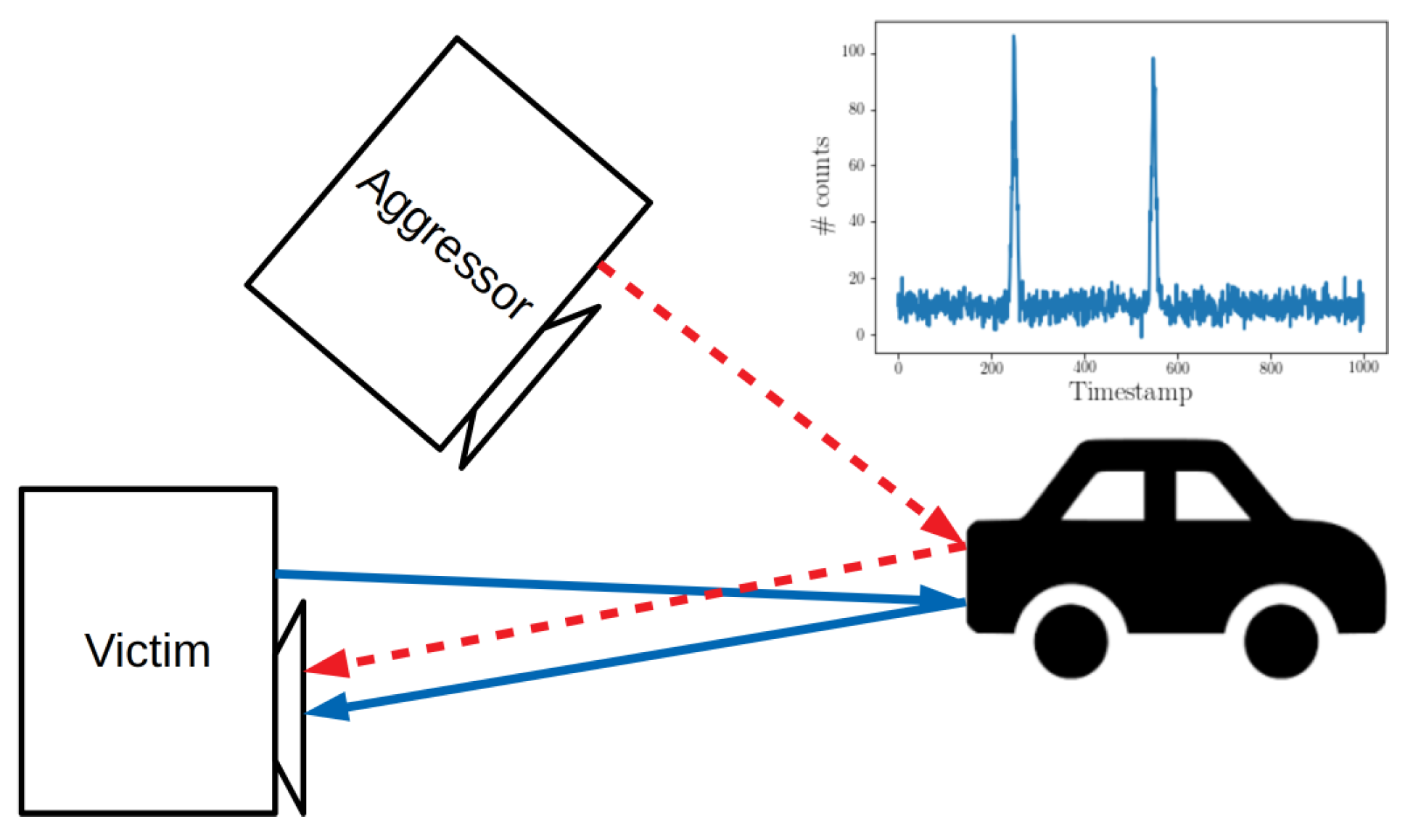
A third-party device able to generate optical interference is defined as an aggressor, regardless of the intent of the interference action. Figure 3 illustrates the concept of optical interference between two cameras imaging the same object.

The worst possible case for a TCSPC LiDAR victim is to operate in an environment with an aggressor that uses the same functional parameters (emission wavelength, pulse repetition frequency, and pulse duration). In this case, the photons of the aggressor will appear as correlated to the victim. The corresponding pixel events will build up in a second histogram peak with an unknown delay that is dependent on the phase shift between the PRFs of the two devices and the difference in length between the victim–target–victim and aggressor–target–victim optical paths.

Once in the histogram, the aggressor peak is indistinguishable from the victim’s peak. This uncertainty in the interpretation of the LiDAR data is a source of risk as it is impossible to differentiate between a real object and an artifact of interference.

5. Interference Suppression

The FLISS technique allows a TCSPC LiDAR to operate safely and free from optical interference in the presence of an arbitrary number of aggressors without requiring any central coordination or communication between devices.

Optical interference suppression is achieved by the addition of discrete random delays to the generation of the laser pulse of the victim. The interval between two laser pulses of the victim then becomes

$$\Delta T_{p,v}=\mathrm{T}+T_{\mathrm{rnd}}=\frac{1}{\mathrm{PRF}}+T_{\mathrm{rnd}},$$

(3)

where $\Delta T_{p,v}$ is the interval between two consecutive laser pulses of the victim, $\mathrm{PRF}$ is the nominal pulse repetition frequency of the victim, $\mathrm{T}$ is the period of laser repetition at the nominal $\mathrm{PRF}$, and $T_{\mathrm{rnd}}$ is a discrete random variable describing a positive delay with a different value for every generated laser pulse. Under this definition, the victim implementing FLISS will operate at an effective average PRF that is lower than the nominal PRF and is defined as

$${\mathrm{PRF}}_{\mathrm{eff}}=\frac{1}{\mathrm{T}+E\left(T_{\mathrm{rnd}}\right)},$$

(4)

where $E\left(T_{\mathrm{rnd}}\right)$ represents the expected value of the random variable $T_{\mathrm{rnd}}$.

The next laser pulse is therefore fired at $T_{p,v}=T_0+T_{\mathrm{rnd}}$, where $T_0$ is the time at which the laser would normally have fired according to its nominal PRF. Due to the delay in the firing of the laser, all signal-related pixel activity will also be delayed by an equal amount ($T_{\mathrm{pixel}}=T_{ToF}+T_{\mathrm{rnd}}$). The statistics of events induced by ambient light and noise won’t change as a consequence of the introduction of $T_{\mathrm{rnd}}$. The final timestamp is calculated as the difference of the previous quantities, therefore

$$T_{\mathrm{ts}}=T_{\mathrm{pixel}}-T_{p,v}=T_{ToF}+T_{\mathrm{rnd}}-T_0-T_{\mathrm{rnd}}=T_{ToF}-T_0.$$

(5)

It is shown that the victim is in principle not affected by $T_{\mathrm{rnd}}$, regardless of its value and temporal evolution. The delay $T_{\mathrm{rnd}}$ is chosen randomly in a bounded interval $(0,T_{\mathrm{MAX}}]$, where $T_{\mathrm{MAX}}$ is finite.

The absolute timing of the laser pulses generated by the aggressor is not influenced by the random delay $T_{\mathrm{rnd}}$, therefore the timestamps generated by the victim from aggressor activity can be defined as

$$T_{\mathrm{ts},\mathrm{a}}=T_{ToF,a}-T_0-T_{\mathrm{rnd}},$$

(6)

where $T_{ToF,a}$ is the ToF from the aggressor to the victim, passing by the target object. It is shown that each aggressor timestamp is shifted in the victim’s reference frame by an amount equal to the variable quantity $T_{\mathrm{rnd}}$, which is not canceled out for the aggressor.

Thanks to the variable nature of $T_{\mathrm{rnd}}$, aggressor timestamps can be distributed across the entire measurement range of the victim, effectively decorrelating the aggressor signal. The quality and performance of the decorrelation depend on the statistical properties of the temporal evolution of $T_{\mathrm{rnd}}$.

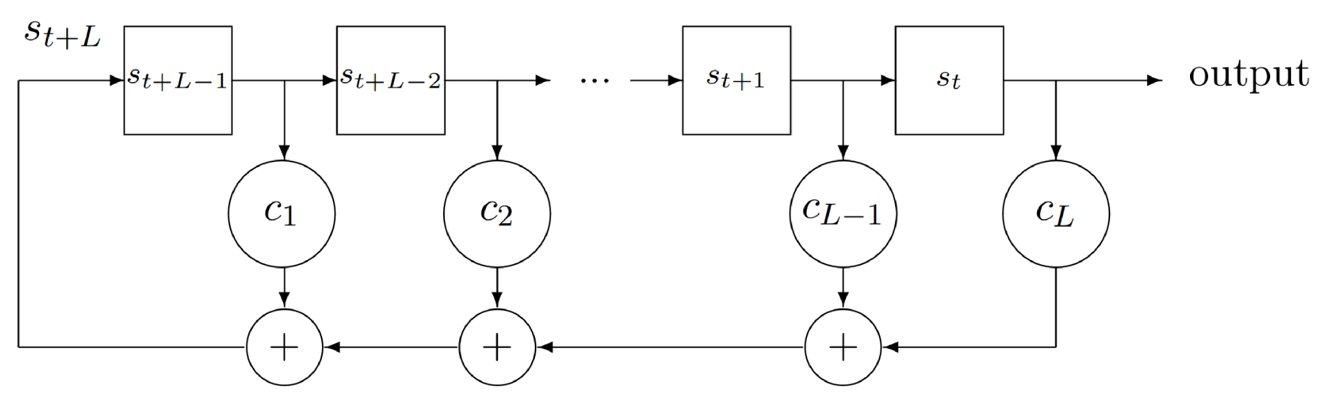
The random delay $T_{\mathrm{rnd}}$ can be generated in a variety of ways. For simplicity of implementation and explanation, we chose to generate the pseudorandom delays using a well-known linear feedback shift register (LFSR) structure [29,30], exemplified in the high-level diagram of Figure 4. The statistical properties of the pseudorandom sequence generated by an LFSR depend on the register’s length L and on the position of the register feedback taps, defined by the feedback polynomial

$$P\left(X\right)=1-\sum _{i=1}^L{c}_i{X}^i,$$

(7)

where $c_i$ are the feedback coefficients of the LFSR. In particular, we restricted ourselves to the use of LFSRs whose characteristic polynomial, defined as

$$P^{*}\left(X\right)=X^{L}P(1/X)=X^L-\sum _{i=1}^L{c}_i{X}^{L-i},$$

(8)

is primitive. LFSRs with primitive characteristic polynomials generate maximum-length sequences (m-sequences) that guarantee that all possible register combinations will be reached before the sequence repeats.

In our implementation, $T_{\mathrm{rnd}}$ can be chosen from a finite list of candidate delays steps D defined as

$$D=R·T_{\mathrm{clk}},$$

(9)

where $R\in [0,1,\dots ,2^L-1)$ is the set of all possible states of the LFSR of length L, and $T_{\mathrm{clk}}$ is the period of the system clock.

6. Experimental Results

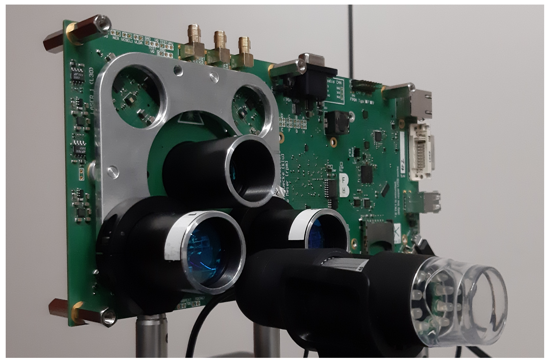
The experimental setup is based on a custom-designed field-programmable gate array (FPGA) board (Figure 5) equipped with a custom SPAD sensor with on-chip TDCs (center) and four independent pulsed VCSEL array illuminators, two of which (lower left and lower right) were used in this work. A conventional webcam has been added to the setup to simplify the optical alignment.

Table 1. Summary of the specifications of the system.

Parameter	Conditions	Value	Units
Technology node	CMOS image sensor (CIS)	180	nm
Pixel pitch		30	µm
Pixel array size		60x1
TDC LSB		50	ps
TDC range		408	ns
Victim/aggressor laser wavelength		850	nm
Victim/aggressor laser bandwidth		<5	nm
Victim/aggressor pulse duration	full-width half-maximum (FWHM)	2.1	ns
Nominal pulse repetition frequency (PRF)		1	MHz
System clock		80	MHz
Laser power	continuous wave (CW)	8	W
Laser divergence		18	deg
Target distance		4.0	m
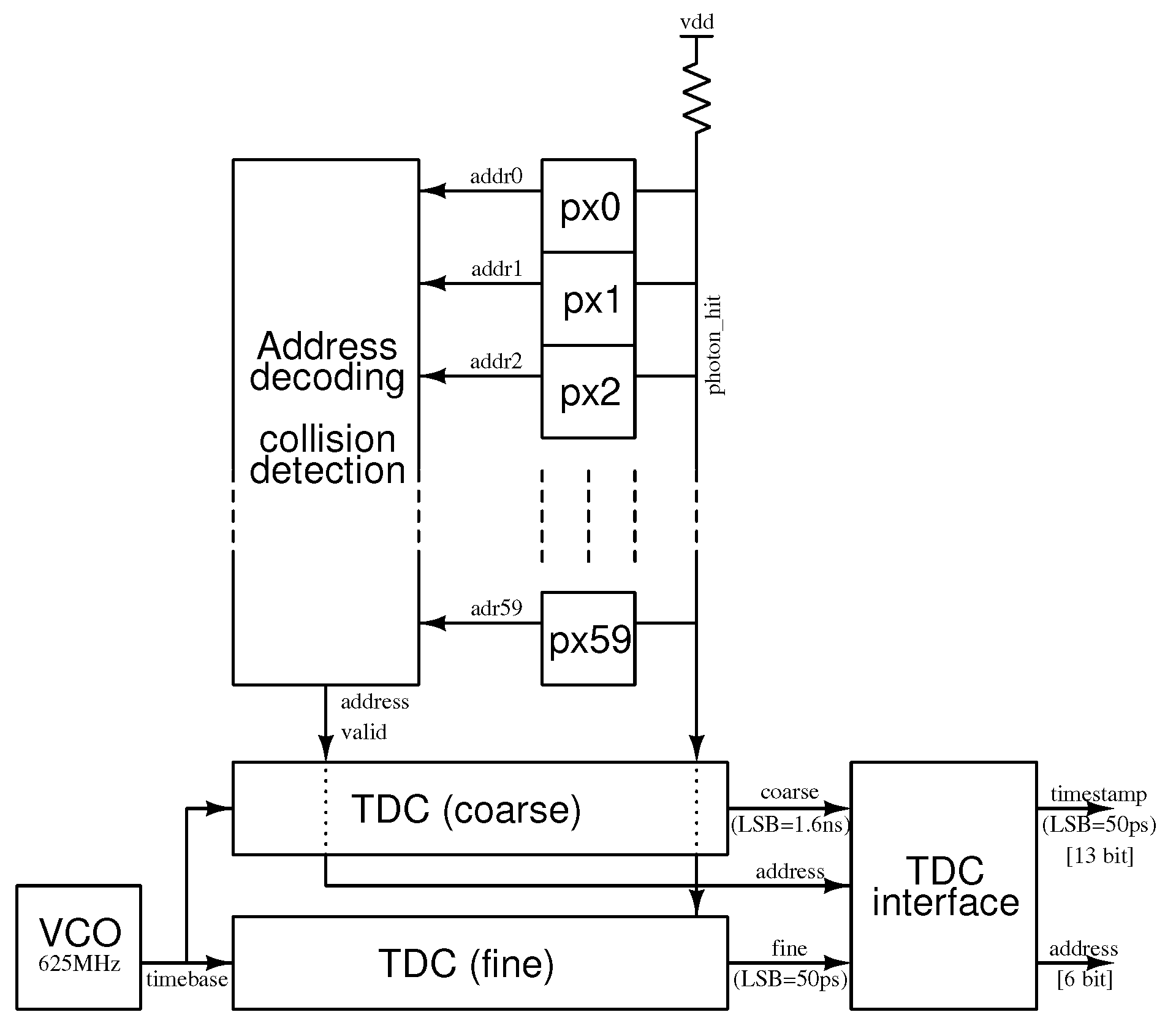
Target reflectivity	Estimated	0.8

summarizes the key specifications of the system, and Figure 6 shows an overview of the high-level architecture of the detector chip.

The victim and the aggressor were installed in front of the same target (a white wall) and operated indoors. When active, the aggressor was assigned a fixed time offset $t_a=75\mathrm{ns}$ to emulate a relative distance to the victim. The aggressor was configured to operate at the effective PRF of the victim to actively try to inject an artifact into the victim’s histogram. All measurements were taken from a single pixel and a single TDC of the sensor. For each experiment, 300 identical acquisitions were recorded to capture statistical fluctuations in the data. Unless otherwise noted, all acquisitions were repeated for three values of integration time $T_{\mathrm{int}}\in [10\mathrm{ms},30\mathrm{ms},100\mathrm{ms}]$.

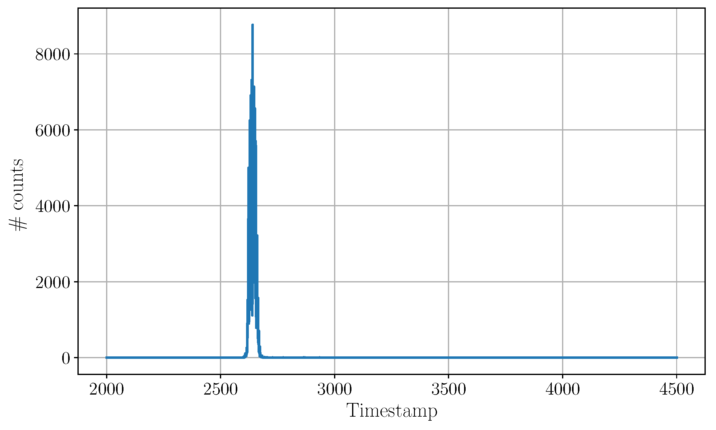
Figure 7 shows the histogram of the victim in absence of any aggressor activity. Under the measurement conditions indicated in Table 1 and with an integration time of $T_{\mathrm{int}}=100\mathrm{ms}$, the victim expresses a single histogram peak with $T_{\mathrm{FWHM},v}=1.65\mathrm{ns}$ located at $T_{\mathrm{ToF},v}=132.1\mathrm{ns}$.

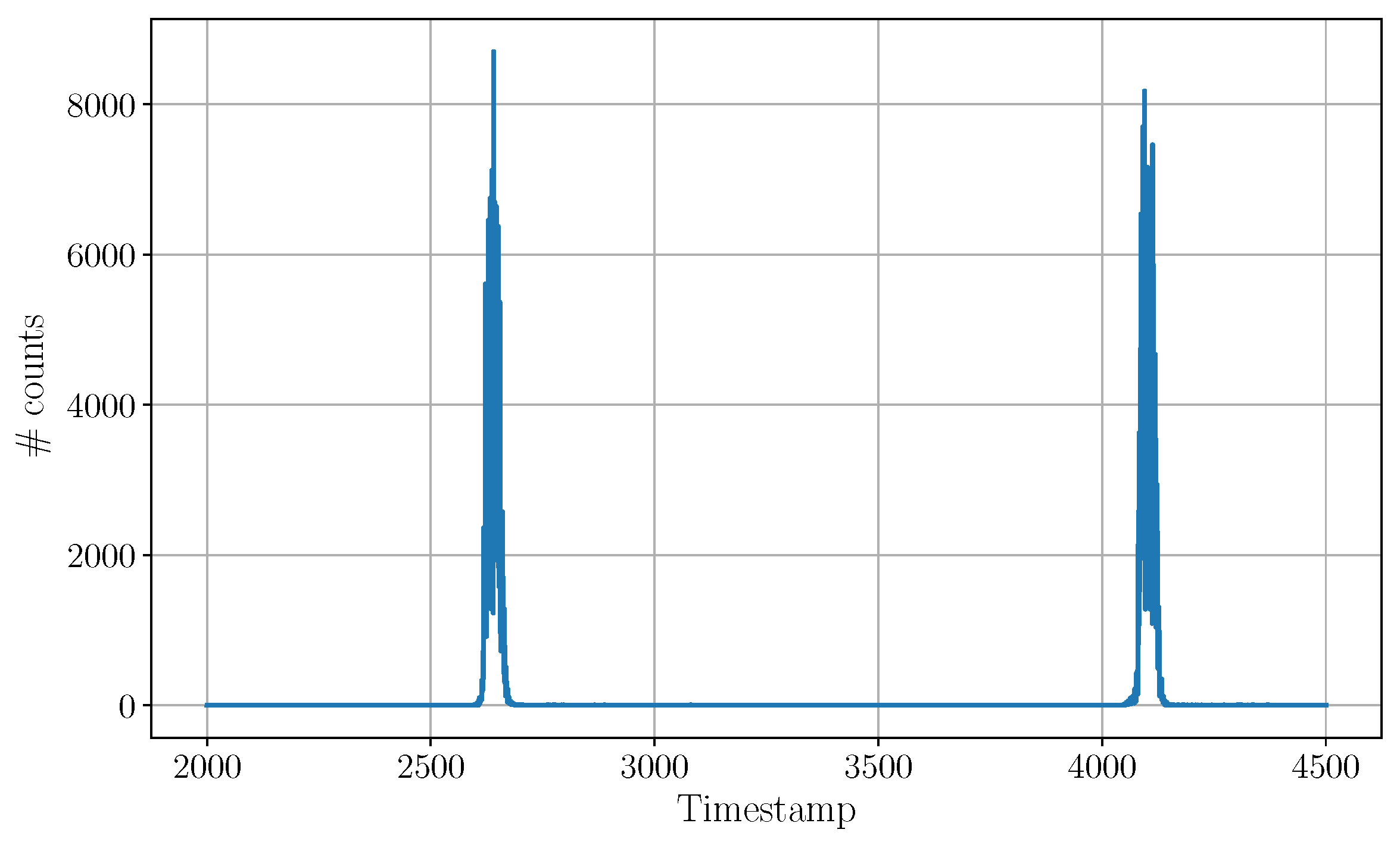
The aggressor was then activated and configured to run at the same PRF as the victim. The plot in Figure 8 shows the histogram measured by the victim in this case. A second peak at $T_{\mathrm{ToF},a}=204.8\mathrm{ns}$ appears due to the aggressor interfering with the victim.

In the following measurement, the optical interference suppression characteristics of the FLISS method were investigated. In all previous measurements, the time interval between two consecutive laser pulses was always and unconditionally equal to $\frac{1}{\mathrm{PRF}}$. Now, each laser pulse of the victim is delayed by a random number of system clock cycles compared to its scheduled time. An LFSR with a primitive polynomial is used to generate a maximum-length pseudorandom sequence of delays. Four LFSRs were used, with length $L\in [3,4,5,6]$ bits, and the suppression ratio was measured for three different values of integration time (Figure 9). The suppression ratio is defined as

$$S=10log\frac{P_v}{P_a}\left[\mathrm{dB}\right],$$

(10)

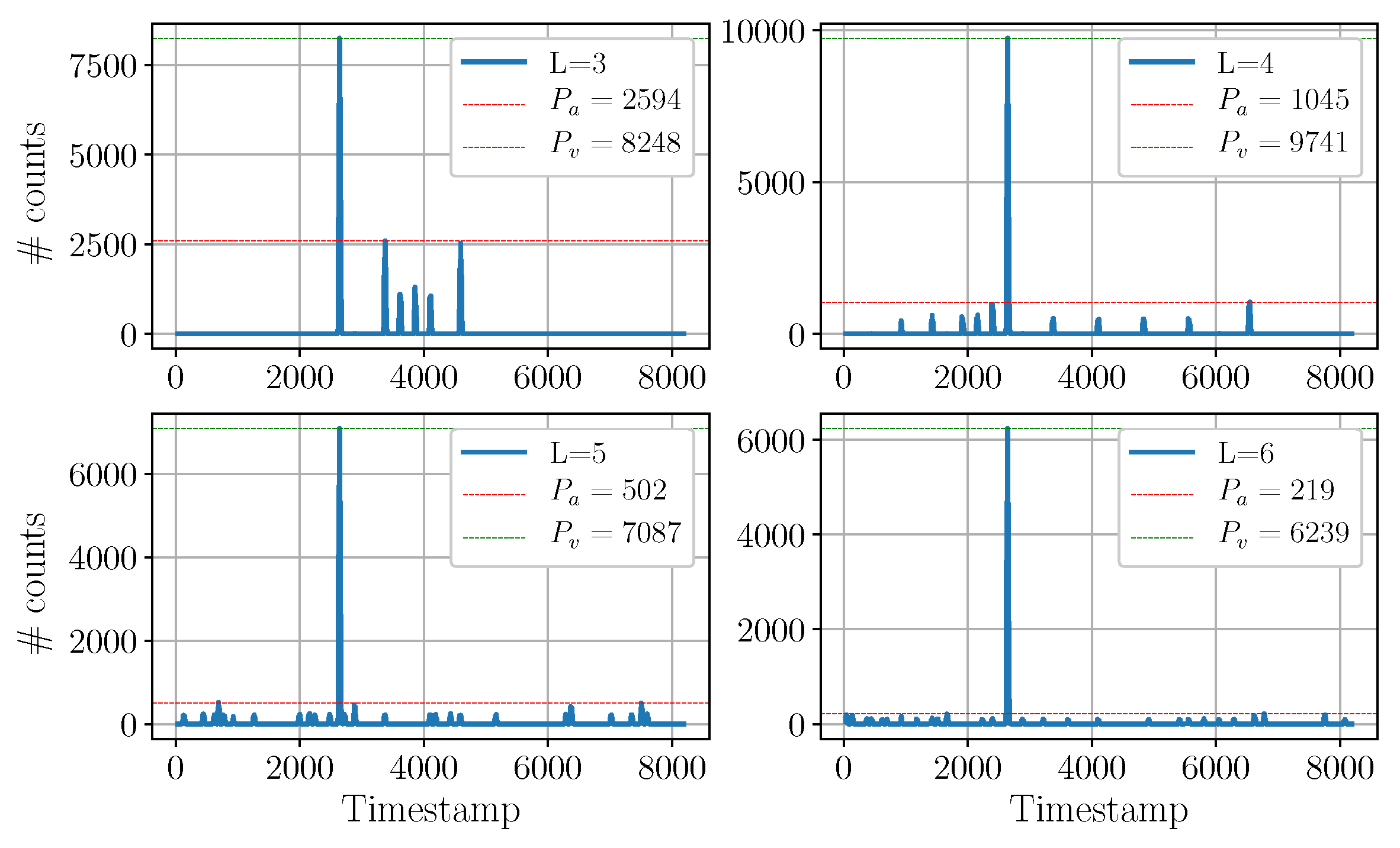
where $P_v$ is the histogram peak value of the victim, $P_a$ is that of the aggressor, and S is the suppression ratio expressed in dB. Figure 10 illustrates the effect of the suppression on the histogram of the victim.

It is shown that the suppression ratio improves with the increasing length of the LFSR, reaching a maximum measured suppression of $35\mathrm{dB}$ using complete sequences. This is expected, as longer LFSRs produce longer sequences with a larger set of delay steps. The suppression appears to be worst for short LFSRs and long integration times. This occurs when $R_L·F_{\mathrm{clk}}^{-1}<<T_{\mathrm{int}}$, where $R_L$ is the length of the m-sequence generated by the LFSR of length L, $F_{\mathrm{clk}}$ is the system clock frequency, and $T_{\mathrm{int}}$ is the integration time. In this case, the repetition of the same pseudorandom sequence of delays during the same acquisition introduces deterministic systematic patterns in the scrambling of the aggressor.

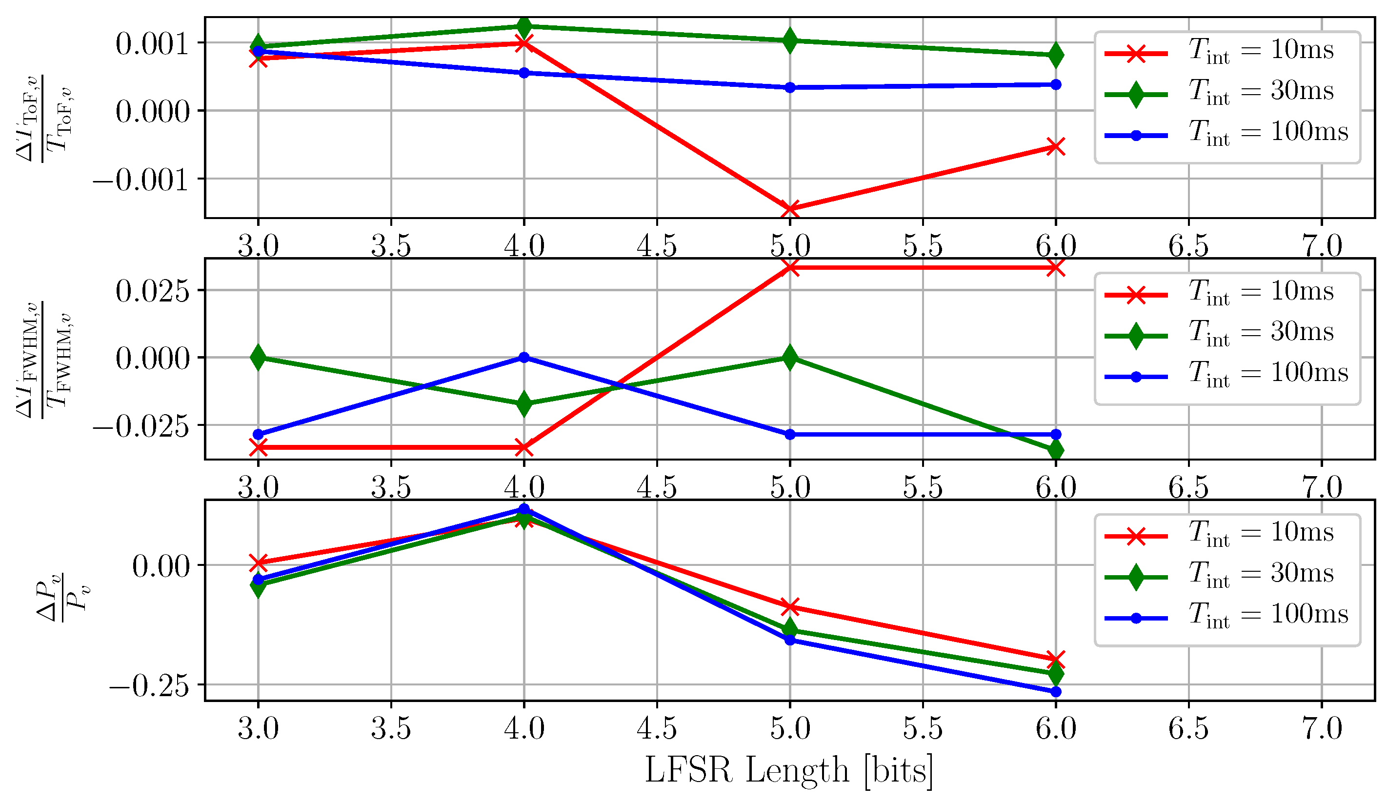
The use of the FLISS technique is shown to have minimal impact on the characteristics of the victim’s output. Figure 11 illustrates the variation of three key quantities (the intensity of the TCSPC peak $P_v$, the measured time-of-flight $T_{\mathrm{ToF},v}$, and the width of the peak $T_{\mathrm{FWHM},v}$) relative to a reference acquisition taken in absence of interference. The experiment shows that applying FLISS does not substantially impact the measurement of the time-of-flight. Similarly, the full-width at half-maximum (FWHM) of the peak shows a maximum deviation of 3%, which is very tolerable from the point of view of signal integrity. The relative variation of the TCSPC peak intensity $P_v$ stays small and close to 0 for $L\le 4$. For larger values of L, a consistent and expected decline has been observed. The reason is to be found in the probability of accidentally shifting aggressor activity right before the time of arrival of the signal peak. Given the parameters of the system, including the distance between victim and aggressor and the mutual phase shift of their PRFs, there will be a value of L after which the activity of the aggressor will start to be shifted in the vicinity of the time of arrival of the signal. When that happens, the shifted aggressor events will likely occupy the sensor and compete with signal photons. It is exactly the same effect we observe when the LiDAR imager interacts with uncorrelated signals such as sunlight. Figure 10 provides a good example to visualize this concept. This is another evidence that for $L\ge 4$, the aggressor will lose its correlation to the victim and will start behaving like ambient light for all intents and purposes.

It is important to note that increasing the length L of the LFSR has the undesirable consequence of reducing the effective PRF of the system.

Table 2. This table provides a correspondence between the length of the LFSR and the effective PRF of the system running at $80\mathrm{MHz}$ and using complete m-sequences.

$\mathit{L}\left[\mathbf{bits}\right]$	${\mathbf{PRF}}_{\mathbf{eff}}$
3	$963.9\mathrm{KHz}$
4	$919.5\mathrm{KHz}$
5	$842.1\mathrm{KHz}$
6	$720.7\mathrm{KHz}$
8	$386.5\mathrm{KHz}$
16	$2.4\mathrm{KHz}$
32	$0.04\mathrm{Hz}$

shows the effective PRF of a system running at a nominal PRF of $1\mathrm{MHz}$ and system clock of $80\mathrm{MHz}$, for various lengths of the LFSR.

It is therefore impractical to use long LFSRs in real-time applications.

One way to overcome such a limitation is to use a different random number generator (RNG) architecture that can generate long, non-repeating sequences of small values. In our experiment, this was achieved by applying a modulo operator to the state of a 32-bit LFSR. The modulo was implemented as a bit-mask on the last $W_m$ LSBs of the LFSR, and the width of the bit-mask was selectable in $W_m\in [1,2,3,4,5,6]$. The periodicity of the resulting sequence is determined by the length L of the LFSR, while the maximum applicable delay $T_{\mathrm{d},\max }$ is defined by the bit-mask width $W_m$ and the system clock frequency $F_{\mathrm{clk}}$ according to the relation $T_{\mathrm{d},\max }=(2^{W_m}-1)F_{\mathrm{clk}}$. Figure 12 reports the suppression ratio for a victim using a long LFSR ($L=32$) as a function of the bit-mask width $W_m$.

7. Conclusions and Future Work

This work presents the successful implementation of an optical interference suppression scheme for TCSPC flash LiDAR imagers. By applying the method described in this paper, a TCSPC flash LiDAR can effectively operate in environments shared with devices emitting modulated optical signals of arbitrary shape. This is a critical requirement for LiDAR imagers intended to operate in uncontrolled environments where other LiDAR cameras with various architectures and characteristics are expected to be present and active. The robustness of this method against intentional attacks depends on the ability of the aggressor to predict the emission time of each laser pulse of the victim. The method presented in this paper is independent of the specific RNG used. In this paper, we chose to implement a fixed m-sequence generated by a LFSR as an example of an RNG. Hardening the method against intentional interference implies choosing a high-entropy RNG producing long sequences of non-repeating values.

Typical applications in which this work will prove to be useful are automotive sensing for ADAS and autonomous driving, automated guided vehicle (AGV) navigation, and simultaneous localization and mapping (SLAM).

This work is especially significant for flash LiDAR imagers as they are more susceptible to optical interference than scanning LiDARs.

Several directions could be taken to improve and further develop the technique presented in this paper. One interesting possibility to be examined is the extension of this work to include the rejection of MPI self-interference. The authors intend to investigate the properties of alternative pseudorandom number generators (PRNGs) with different statistical distributions and the possibility of using quasi-continuous delay steps, as a necessary measure to enhance the victim’s resilience against intentional attacks.