1. Introduction
Sentence classification is a fundamental problem in natural language processing (NLP) which aims to organize a very large amount of textual information into groups so that users can access this bulk information with so much ease. Sentiment analysis, a sub-task of sentence classification, tries to identify and categorize opinions expressed in a piece of text to determine the overall contextual polarity. Because human language is complex and there are irregularities in usage, sentence classification is generally a difficult task which requires very careful modeling and analysis.
Previous research on sentence classification or sentiment analysis relied on using different methods ranging from non-neural network based approaches like topical categorization and knowledge based models to neural network based techniques. With the immense amount of research and improvements in deep learning, however, recent works depend mainly on convolutional neural networks (CNNs) and recurrent neural networks (RNNs)—the two notable networks used in various kinds of computer vision and NLP tasks.
While CNNs are usually employed in the area of image processing and analysis, Kim [
1] introduced the use of CNNs for sentence classification and the results are very promising especially when pre-trained word-vectors are available. Even though CNNs enjoyed enormous popularity in the deep learning community, the recent introduction of capsule networks (CapsNets) by Hinton et al. has opened a lot of investigation into the structure of CNNs, especially the pooling operation which causes loss of the important spatial relations between different features [
2,
3].
The motivation for CapsNets stems from the fact that neural networks needed better modeling of spatial relationships among parts instead of modeling the co-existence disregarding relative positioning. CapsNets accomplish this,
capturing of spatial information, by using a set of nested layers in a network called capsules and implementing an algorithm called routing-by-agreement. It is also reported that CapsNets can achieve better results for various kinds of image analysis tasks and are better in resisting adversarial attacks than their CNN counterparts [
3]. Replacing CNNs by CapsNet, which can adequately capture the spatial relations between features, has higher potential for a better representation and understanding of a given NLP task. This performance improvement by using CapsNet for text classification is made evident by recent works of Zhao et al. [
4] and Kim et al. [
5].
In this work, which is an extension of work presented in [
6], we present a CapsNet-based model designed for sentence classification, sentiment analysis in some cases, using a Word2vec model as the vector encoding technique. We trained the proposed CapNet architecture in two successive phases for optimal performance. First, we did a normal training of the model using a
glorot uniform kernel initializer which was then followed by retraining of the same model with reinitialized weights of the CapsNet module in the second phase. The details of the network and approaches used are presented in
Section 3 and
Section 4. Also presented is a comparative analysis of our CapsNet model against other models including CNNs and RNNs. The results of our experiment show that our well-tuned CapsNet model outperforms CNN models and can be a good, sometimes better and cheaper, substitute of much slower RNN-based models used in sentence classification.
2. Related Work
Over the years, a large body of research work was conducted on sentiment analysis, or more generally on sentence classification tasks. Earlier non-neural network based approaches focused on topical categorization, attempting to sort documents according to their subject matter. However, applications like business intelligence or other product review require more sophisticated and in-depth analysis of the opinions presented than topical categorization. Other approaches have partially been knowledge-based, using linguistic heuristics or a pre-selected set of seed words as in the work by Pang et al. [
7]. The authors used Naïve Bayes classification, maximum entropy classification and support vector machines (SVMs) to perform sentence classification on a movie reviews (MR) dataset, producing moderate results. The problem with these approaches is that they require a priori knowledge or pre-selected seed words.
Other popular approach for sentence classification, question classification specifically, is to use rule-based classifiers. Silva et al. [
8] used a rule-based classifier with an SVM to classify Text REtrieval Conference (TREC) questions. Even though they were able to record state-of-the-art performance using this approach, the use of manually built patterns makes it unfit for practical uses, especially when there are large and varied datasets. In the work by Hermann et al. [
9], semantically meaningful vector representations from sentences and phrases of variable size were extracted using combinatorial category grammar (CCG) operators and each of these vector representations were fed to an autoencoder function for classification. Genetic algorithms (GAs) were also used for automatic classification of text sentiment in the work by Dufourq et al. [
10]. In their work, which the authors referred to as a genetic algorithm for sentiment analysis (GASA), they proposed a GA approach to classify sentences by optimizing unknown words as either a sentiment or an amplifier word which was able to outperform certain systems.
Kim [
1] proposed a shallow CNN network for sentence classification which has single convolution and pooling layers. The author compared the performance by applying random embedding (CNN-rand), pre-trained Word2vec embedding (CNN static), and pre-trained Word2vec embedding with fine-tuning using back propagation (CNN non-static) on common datasets. The reported results show superior accuracy for most datasets used in the experiment. Moreover, the author argued that a pre-trained Word2vec model can be used as a general-purpose choice for text embedding. Another notable work for sentence modeling is a work by Kalchbrenner et al. [
11] which used a deep CNN with dynamic k-max pooling that can handle sentences of varying lengths. Cai et al. [
12] also adopted a CNN for multimedia sentiment analysis consisting of texts and images. Yet another CNN architecture by Zhang et al. [
13] was used for text understanding from character-level inputs all the way up. While most CNN models for text classification are shallow, Conneau et al. at Facebook-AI [
14] came up with a very deep CNN architecture showing that the performance of this model increases with the depth. Though these CNN based models produced notable results, we proved that a well tuned CapsNet based models can do better.
By combining a recurrent structure from RNNs and max-pooling from CNNs, Lai et al. [
15] proposed an RCNN model for text classification which produced good results. The recurrent structure, a bi-directional RNN with word embeddings, is utilized to capture contexts in both directions of a given word and the output is propagated through a max pooling layer. The long-short-term-memory-network (LSTMN) by Cheng et al. [
16] was implemented to perform shallow reasoning with memory and attention. This work extended the LSTM architecture with a memory network in place of a single-memory cell which enables adaptive memory usage during recurrence with neural attention. The LSTM-RNN model by Le and Zuidema [
17] and the bidirectional LSTM model with 2D max-pooling by Zhou et al. [
18] also reported great classification accuracy.
Recent works by Zhao et al. [
4], Kim et al. [
5], Xiao et al. [
19], Srivastava et al. [
20] and Yequan et al. [
21] employed CapsNets as the core network for text classification. Zhao et al. [
4] adopted an ensemble of capsule layers whose output is fed to capsule average pooling layer to produce the final results. In their work, they modified the routing-by-agreement algorithm given in [
3] by using
Leaky-Softmax and
coefficient amendment. The results presented show a great improvement over previous CNN-based works. Similarly, Kim et al. [
5] presented a text classification with CapsNet-based architecture which uses an ELU-gate unit before the convolutional capsule layer. The authors experimented on both the dynamic routing and its simplified version they referred to as
static routing. They argued that the simplified
static routing produces superior results to dynamic routing for text classification with respect to accuracy and robustness of classification. Xiao et al. [
19] implemented CapsNets for text classification with multi-task learning. In multi-task learning, sharing as much knowledge between tasks while routing features to the appropriate tasks has been a challenge. The routing-by-agreement in CapsNets has the ability to cluster features that can help to solve the inherent problem of discriminating features for each task in multi-task learning. For this purpose, a modified routing algorithm called task routing was proposed to replace the dynamic routing algorithm so that choosing between tasks may be possible. CapsNets were also implemented with RNN and its variants for text classification tasks. Yequan et al. [
21] used a combination of capsules and RNN for sentiment analysis on MR, Stanford Sentiment Treebank (SST) and Hospital Feedback datasets where all word vectors were initialized by
Glove. In a similar fashion, Srivastava et al. [
20] designed a CapsNet with the LSTM to identify toxicity and aggression in comments.
In this paper, inspired by the success of CapsNets, we present a novel architecture designed for sentence classification, sentiment analysis in some cases, based on CapsNets. Unlike the approaches followed in the above works, we resort to using a cascade of simple convolution operations in parallel before the capsule layer to reduce the high dimensional data into lower dimensions and to encode different features using varying kernel sizes. The cascade of parallel convolution layers is implemented with relatively larger kernel sizes compared to [
4,
5,
19], as larger kernel sizes can be useful to incorporate more information with large receptive fields. While multi-task learning was employed in [
19] to increase the training data size by sharing knowledge among tasks, we implemented a much cheaper alternative using the
Word2vec model for data augmentation, in addition to its usual use of encoding text into vectors, to increase our dataset size. Even though combining CapsNets and RNNs in [
20,
21] exhibits encouraging results, the added use of RNNs makes them more complicated compared to the approach we proposed here. On top of that, since CapsNets can capture contexts and encode the sequences well, the benefits one can get by incorporating RNNs with CapsNet would be of marginal importance. Authors in [
5] argued that, due to high variability in sentence construction, the model should be flexible enough to accommodate modifications such as changing the order of words. One of the reasons why they chose static routing over dynamic routing was to bring about this flexibility. Even though this claim may be valid at times, we argue that the exact order of words plays an important role in the overall meaning of a sentence as changing the order of words in a sentence usually results in a completely meaningless sentence or another sentence with a totally different meaning. This was confirmed by performing a number of experiments using normal and shuffled input test data and comparing the accuracy of each experiment and visualization of the outputs at different layers of our network, the details of which are given in
Section 4. Therefore, in order to keep this spatial information in a sentence, we want our routing algorithm to be able to retain this information as much as possible. For this reason, we stick to using dynamic routing as the preferred routing-by-agreement algorithm. Our model contains different kinds of preprocessing operations like tokenization, text embedding and data augmentation. Details of these operations are given in
Section 3. The overall contributions of our paper can be summarized as follows:
A model with a state-of-the-art classification performance
A model that can capture the correct sequential order of words in a sentence
A model with relatively low cost compared to other state-of-the-art models and
A model where we introduced the use of Word2vec model as an alternative data augmentation technique in the area of text analysis.
In summary, we propose a model designed for sentence classification using CapsNets. We underline that keeping the order of words is crucial to correctly understanding the meaning of sentences in most languages. The choice of CapsNets guarantees this as the capsule layers are designed not to disturb the spatial relations. Word2vec is used as the preferred method of text encoding and data augmentation.
3. Proposed Model
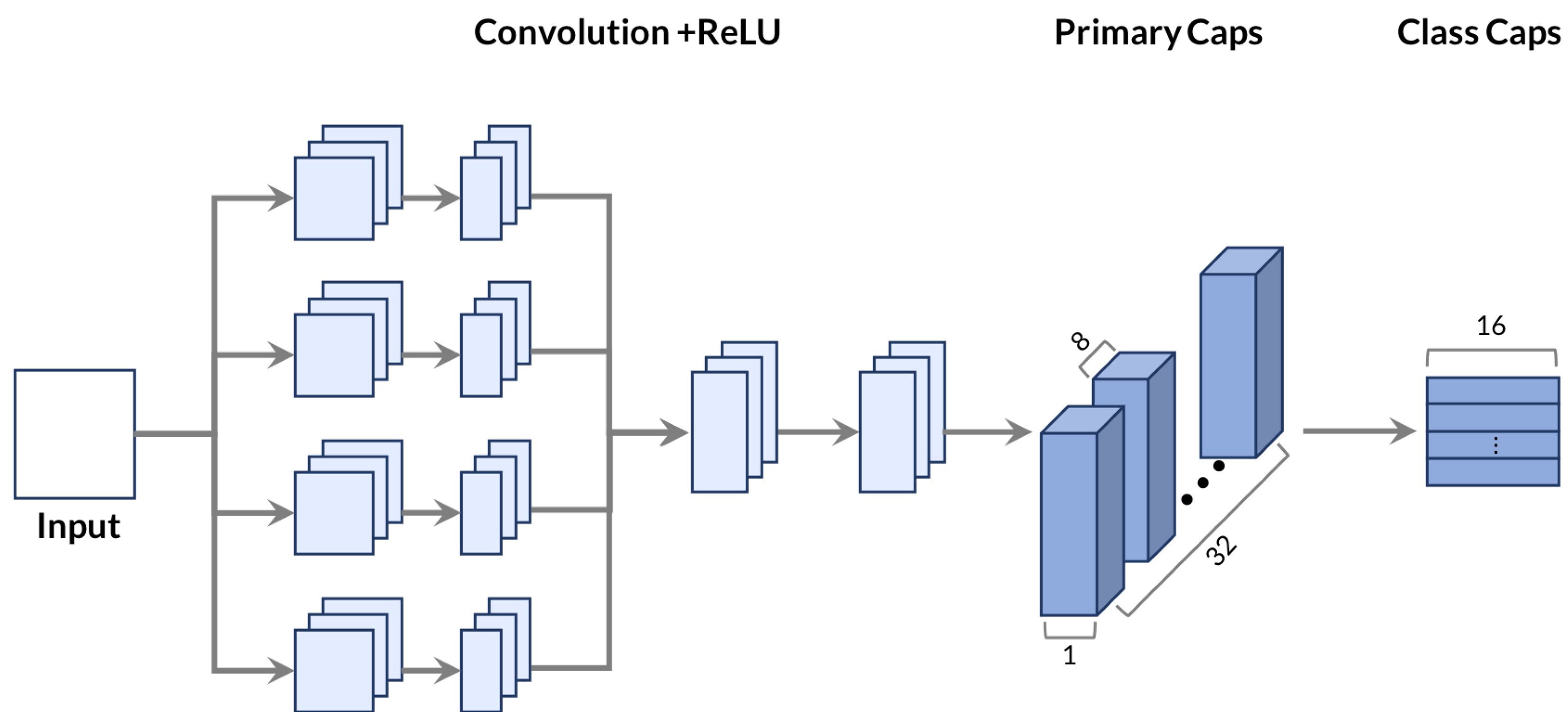
The CapsNet architecture proposed in this paper is given in
Figure 1. CapsNet introduced the concept of capsules which are a group of neurons whose activity vector represents different parameters of a specific entity [
3]. The magnitude of a specific vector in a capsule represents the probability of detecting a feature and its orientation represents its instantiation parameters. In CapsNet, the output of a given capsule is sent to an appropriate parent in the layer above using an algorithm called dynamic routing by agreement [
3]. In addition to having the capability to maintain all spatial information, capsules also show far more resistance to white box adversarial attacks than standard convolutional neural network. The basic CapsNet given in [
3] contains a convolution layer, another convolution layer named primary capsules layer, and the final layer called digital capsules layer.
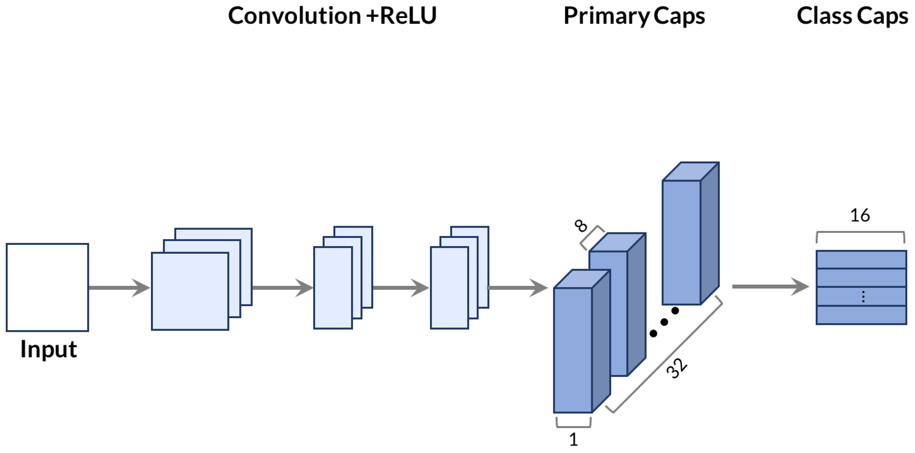
We tested several architectures including CapsNet with only a single-layer convolution, two-layer convolution, and three-layer convolution, all with and without the parallel convolution operations, one example among which is shown in
Figure 2. The architecture which produced the best results (as much as 3–4% increase in accuracy compared to others) is the one given in
Figure 1. Another attempt was made to use parallel primary capsule layers after every parallel convolution block. The results of this were compared to the network given in
Figure 1 and there was no noticeable difference and hence we decided to use the network with the least complexity given in
Figure 1.
As it can be seen from
Figure 1, the first few stages contain an array of convolution layers each with different kernel sizes to extract varying features from the input dataset. Prior to connecting the input to the proposed network, the input data have to pass through a number of preprocessing stages. These preprocessing stages are summarized below.
3.1. Preprocessing
In order to replace each word in a given sentence by its vector representation, the input sentence has to be broken down into words. This is achieved through a process called tokenization. We used a simple string cleaning or stripping technique similar to the one used in [
1] as a tokenizer. After the tokenization process, the result is passed to data augmentation, which is followed by word embedding. For both data augmentation and word embedding purposes, we relied on the publicly available pre-trained Word2vec model by Mikolov and colleagues [
22]. This Word2vec model with an embedding dimension of 300 was pre-trained on a huge Google News dataset of around 100 billion words for a vocabulary of three million words and phrases.
For different datasets and different sentences within a given dataset, the sentence length varies widely. Since the network architecture requires an input with fixed dimensions, we apply zero padding to the sentences so that every sentence in a given dataset has the same length.
3.2. Sentence Model
In
Figure 1, the input stage represents a sentence of the form
, where each
, for
, represents a constituent word for any given sentence and ⊕ represents a concatenation operation. In the 2D representation, a single sentence is represented by a vector of dimensions
, where
n is the number of words in the given sentence and
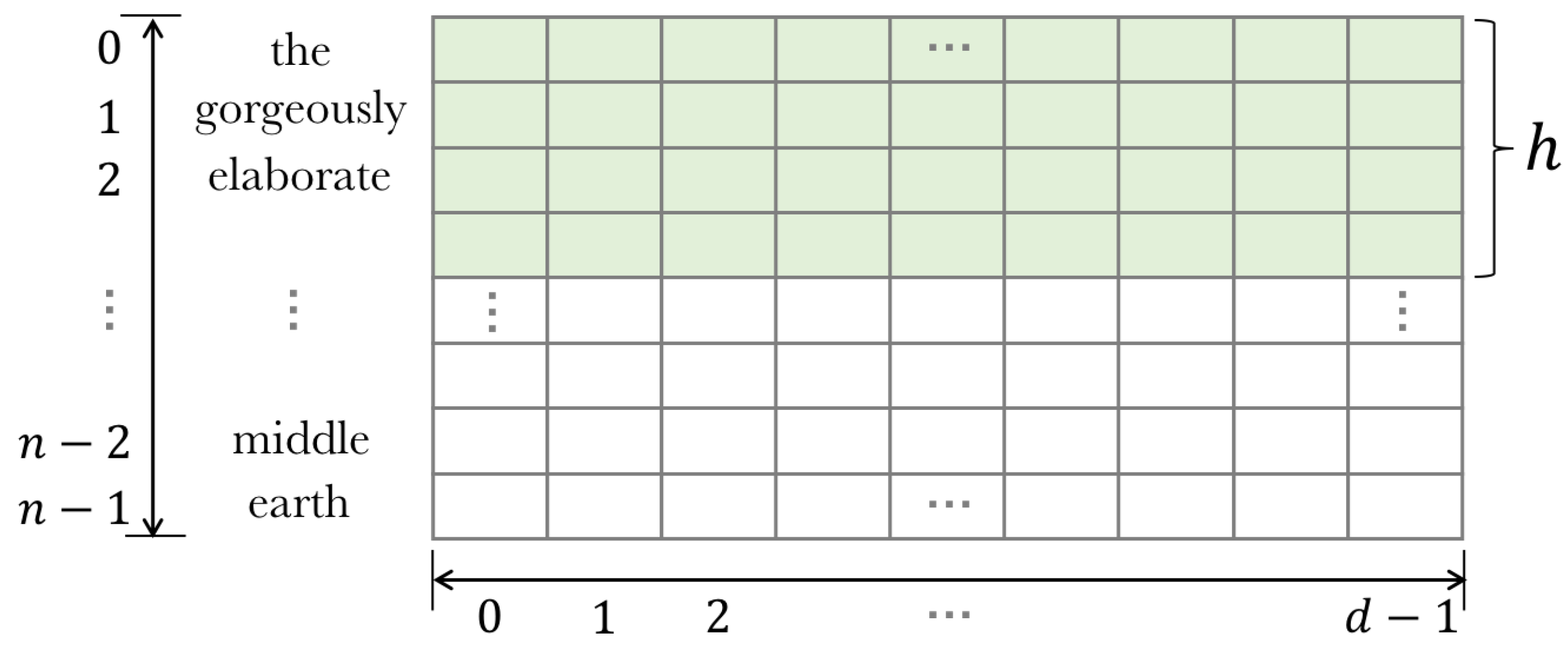
d is the embedding dimension which is 300. In this model, every row represents individual words as can be seen in
Figure 3.
3.3. Convolution Stage
The convolution operation is mainly used to extract features in the given input. As mentioned above, since one row represents one word, we need to apply the convolution operation to the entire column i.e., we must use a sliding window of kernel size—
(see
Figure 3). Here,
h is the number of words we want to use in a single convolution step (N-gram word). Using the convolution operation this way has two advantages: the sequential order of words is kept, and the total number of convolution operations is reduced. This reduces the total number of parameters which in turn will result in increased system speed.
In this convolution operation, a feature
is generated for a given filter
as:
where
, for
, is the generated feature,
is a nonlinear activation function (ReLU used here),
is the filter (we have
m set of those filters),
, for
is the input word vector and
, for
is a bias term. The concatenation of features
forms a column feature vector
F in the first stage convolution.
As can be seen from
Figure 1, a parallel set of convolution operations with varying kernel sizes is utilized. The main reason for using this parallel set of convolution layers is to capture possible word combinations which will form as many specific features as possible.
The results of the second stage parallel convolution operations are then concatenated to produce m column vectors, where m is the number of filters. This output is then made to pass through other two stages of convolution, with dropout in between them, before it is processed in the Primary Caps layer. It should be noted that, in addition to extracting features, the convolution stages help in reducing the dimensionality of the input data. This is desirable as CapsNets work better with low dimensional input.
3.4. Primary Caps Layer
This layer is a standard convolution layer which accepts scalar inputs from the previous convolution layers and produces vector outputs called capsules to preserve the instantiate parameters such as the local order and semantic/syntactic representations of words. In this Primary Caps layer of dimension 8D and 32 channels, features detected by the previous convolution layers produce combinations of features grouped into capsules.
CapsNets replace scalar-output feature detectors with vector-output capsules in this layer and going up to the next layer in the network requires the routing by agreement algorithm. When multiple capsules agree in their vote to a specific capsule in the layer above, that capsule gets activated and results from lower level capsules are propagated to that capsule. This activated capsule will create a cluster of capsules which came from a lower layer and causes the higher-level capsule to output a high probability of observation that an entity is present and a high-dimensional pose.
The routing by agreement mechanism used here is dynamic routing and this mechanism provides a means to connect the Primary Caps Layer with the next layer—Class Caps Layer. If we assume the output of a single capsule (pose vector) is
, it is multiplied by a translation matrix
to produce a vector
. Here, capsule ‘
i’ is in the current layer (Primary Caps Layer in this case) and capsule ‘
j’ is a capsule in the higher level. A capsule in the higher level is fed the sum of the outputs in the lower level (Primary Caps Layer) multiplied with a coupling coefficient
that is calculated during the dynamic routing process:
These coefficients
are calculated using a softmax function and they all add up to one:
where
.
is the initial logits (prior probabilities that capsule
i should be coupled to capsule
j ) and
is the output vector limited to [0, 1] using a squashing function as given below:
The length of the instantiation vector represents the probability that a capsule’s entity is present in the scene. For details of the dynamic routing algorithm, look at [
3].
3.5. Class Caps Layer
The Class Caps Layer is the final capsule layer in this network. This layer accepts values from the layer below through the routing by agreement process. This layer has a capsule of dimension 16D per class and a routing of 3 is used in the iterative dynamic-routing algorithm.
4. Experiments, Results and Discussion
In this section, we report the results of a series of experiments conducted on various datasets using the proposed CapsNet architecture in
Figure 1 and two baseline CNN and LSTM models for comparison. We present a comparison of the accuracy of our CapsNet model with other state-of-the-art models, a visualization of the capsule outputs, and a detailed error inspection in the inference stage.
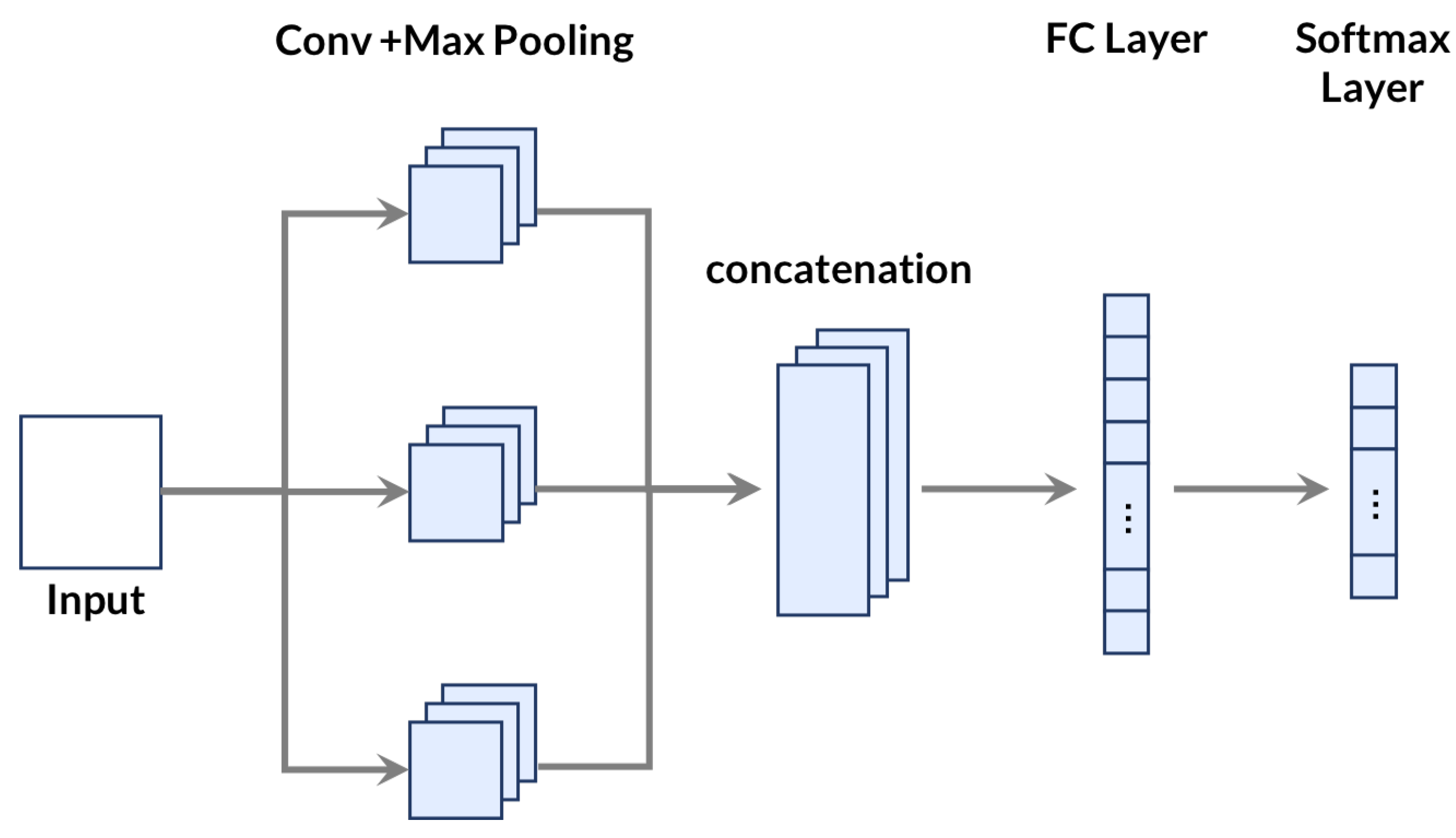
The baseline CNN model is shown in
Figure 4. As the baseline LSTM model, we used Keras’ LSTM model with the following layers: Input layer, Embedding layer of shape (None, Sentence Length, 300), LSTM layer of shape (None, 50) and Dense layer of shape (None, Number of Classes), where ‘None’ refers to the number of samples and ‘50’ is the dimensionality of hidden units/output units in the LSTM network. All of the experiments were performed using Keras with TensorFlow backend in a machine with Intel Core i7-8700 CPU at 3.20 GHz, two GeForce GTX 1080 Ti GPUs and 32 GB RAM.
The datasets used in the experiment are the following and details of these datasets are given in
Table 1.
MR Dataset: movie review dataset (positive/negative review) [
23].
TREC Dataset: 6 class Text REtrieval Conference dataset (Entity, Human, Location, ⋯) [
24].
SST-2 Dataset: modified version of the MR dataset provided on a phrase and sentence level [
25].
Subj Dataset: Subjectivity dataset (subjective/objective sentence) [
26].
MPQA Dataset: contains mostly short news articles from a variety of sources manually annotated for opinion polarity [
27].
In the experiments, data augmentation was used in the training stage. This augmented data were generated by using Word2vec. To generate synonyms for the data augmentation task, WordNet with the help of Natural Language Toolkit (NLTK) was also tried, but Word2vec usually gives more replacement options (synonym words for a given word) than WordNet.
4.1. Baseline Models
The CNN model was implemented with: Adam optimizer with learning rate of 0.001, batch size of 100, dropout of 0.8 and 2500 iterations. Similarly, the LSTM model was implemented with: Adam optimizer with learning rate of 0.001, batch size of 150, dropout of 0.8 and 100 epochs. These hyperparameters were chosen after performing exhaustive experiments to generate best results.
In addition to normal testing, to test whether the networks learn the sequential order of words or not, we test both networks with sentences in test dataset where words have been randomly shuffled. If the network learns the sequential order of words, we expect the accuracy of the network with word-shuffling to be lower than the accuracy of the network with no shuffling. The results of our experiment on these two models are summarized in
Table 2.
As can be seen from
Table 2, for most datasets, the difference in accuracy between normal and shuffled test data for the CNN network is not much compared to that of the LSTM network. From this, we argue that the CNN model didn’t learn the spatial information (the exact order of words) of the input data very well. This is expected as max-pooling in CNN is problematic in keeping the spatial order. In most cases, the LSTM network shows a superior performance to the CNN model. SST-2 dataset is presented in both phrase-level and sentence-level representations. The training is done on both phrase and sentence-levels while the test is performed on sentence-level inputs only.
4.2. CapsNet Model
The proposed CapsNet model was implemented with the following hyperparameters: Adam optimizer with learning rate of 0.001, batch size of 30, routing iteration of 3, and 50 epochs. The choice of these values is based on a time-consuming hyperparameter tuning for best performance.
Except for MPQA and TREC datasets (which have shorter sentence length compared to others), we used the following network parameters:
In the first convolution layer, which contains four parallel convolution layers, the kernel size is (7, 300), (8, 300), (9, 300), (10, 300) with a stride of 1 and the number of filters is set to 64.
In the second convolution layer, which also contains four parallel convolution layers, the kernel size for each convolution layer is (7, 1) with a stride of three and the number of filters is set to 64.
In the third, fourth convolution layers and primary caps layer, the kernel size is set to (5, 1) with stride of 2, 1 and 2 for each layer, respectively.
The primary caps layer dimension is set to 8D with 32 channels and
The Class Caps Layer is set to have a dimension of 16D with rows equal to the number of classes in each dataset.
For MPQA and TREC datasets, for the first convolution layer kernel size is (3, 300), (4, 300), (5, 300) and (6, 300) with stride of 1. In the second convolution layer, kernel size of (3, 1) with stride of 3 is used. In the third, fourth convolution layers and primary caps layer, the kernel size is (5, 1) with stride of 2, 1 and 2, respectively.
Similar to the CNN and LSTM models, in order to test whether the CapsNet learns the sequential order of words or not (if it can resist an adversarial attack), we test the network with normal and shuffled test data. The results of our experiment on this model are summarized in
Table 3.
By examining
Table 3, we can observe the following points. The difference between the last two rows for every dataset is huge compared to that of the CNN model. Since the fourth row is added merely for the purpose of verifying if the network learns the sequential order of words or just the presence or absence of a given word, we can safely say that CapsNets learn the sequential order of words effectively than CNNs. Doing the same comparison between the CapsNet and the LSTM model reveals that both networks exhibit almost similar responses.
In order to check if the architecture given in
Figure 1 with parallel convolution layers performs better than a basic CapsNet architecture without parallel convolution like the one given in
Figure 2, an experiment was done on the MR dataset with normal test data. While we got 83.8% accuracy for the architecture in
Figure 1, we got an accuracy of 79.2% for the one in
Figure 2. This result proves that the network with parallel convolution layers performs better since it can capture more characteristic features of sentences related to their semantic or/and syntactic meanings with multiple kernel sizes.
4.3. 2-Phase CapsNet Training
In an effort to enhance the performance of our model, we performed an experiment on the model given in
Figure 1 using a training procedure we call
2-phase training. In the first phase of training, we initialized the weights of the convolution layers and the translation matrix
of the capsule layer using
glorot uniform initializer while the initial logits
are initialized with zero producing uniform coupling coefficients. We trained the network using the given datasets until best test accuracy was obtained. In the second phase, we trained the network further after reinitializing the translation matrix of the capsule layer and capsules’ coupling coefficients while the trained weights of convolution layers are retained. With these proper initial weight values of the convolution layers, the network could be optimized more by learning features effectively to produce better results. In our experiment, this 2-phase training approach resulted in a slightly better performance than the original single-phase training of the CapsNet model. This 2-phase training approach just requires a small additional training time but provides a high potential to improve the performance without the need of increasing the amount of training data. As a result, this approach can be a good option to train multi-module networks for improved performance in any area of application. Our CapsNet model with this 2-phase training is presented in
Table 4 as 2-phase CapsNet.
In
Table 4, we present a performance comparison of our model with other latest works. In the first four rows, we present results of the above models we used, while in the remaining rows we present the results reported in the corresponding papers.
As it can be seen from
Table 4, while our CapsNet model shows comparable or better results than other networks for most datasets, our 2-phase CapsNet model shows much better results than most models. It is clear from the above results that the proposed CapsNet model can understand text data better than CNN models.
Table 4 further shows that, compared to other CapsNet-based approaches given in [
4,
5,
19], our CapsNet models exhibit superior performance.
4.4. Effect of Kernel Sizes and the Number of Parallel Layers
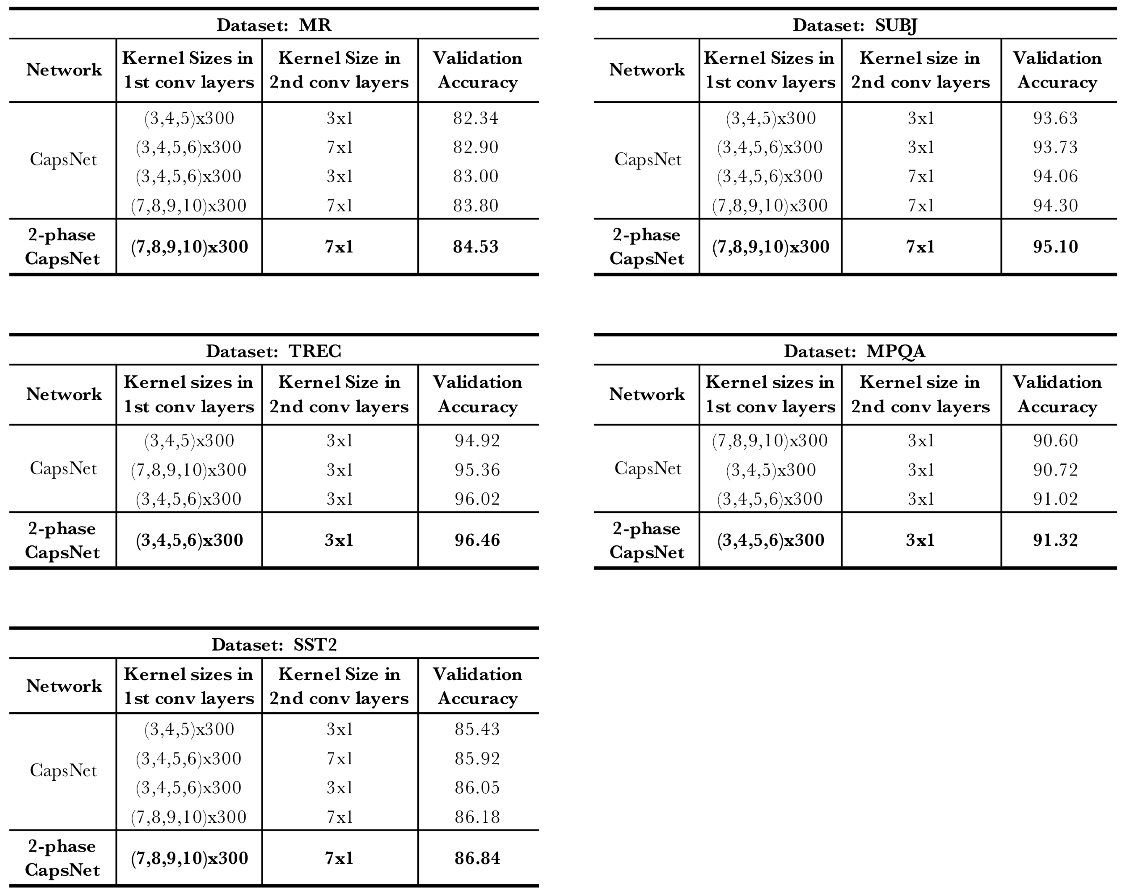
In this section, we present the results of experiments undertaken to investigate the effect of kernel sizes and the number of parallel layers on the performance of the proposed system. As can be seen in
Figure 5, for datasets with slightly longer sentence length like MR, SST-2 and SUBJ using larger kernel sizes in the convolution operations produced better results. In contrast, the network performs better with small kernel sizes in the convolution layers for TREC and MPQA datasets which have relatively shorter sentence lengths. For all datasets, setting the number of parallel convolution layers to four resulted in higher validation accuracy than reducing it to three. In
Figure 5 column 2, (3, 4, 5, 6) × 300 indicates four parallel convolution layers with kernel sizes (3 × 300), (4 × 300), (5 × 300) and (6 × 300). Similarly, (3, 4, 5) × 300 refers to three parallel convolution layers with kernel sizes (3 × 300), (4 × 300) and (5 × 300).
4.5. Looking inside Internal Layers
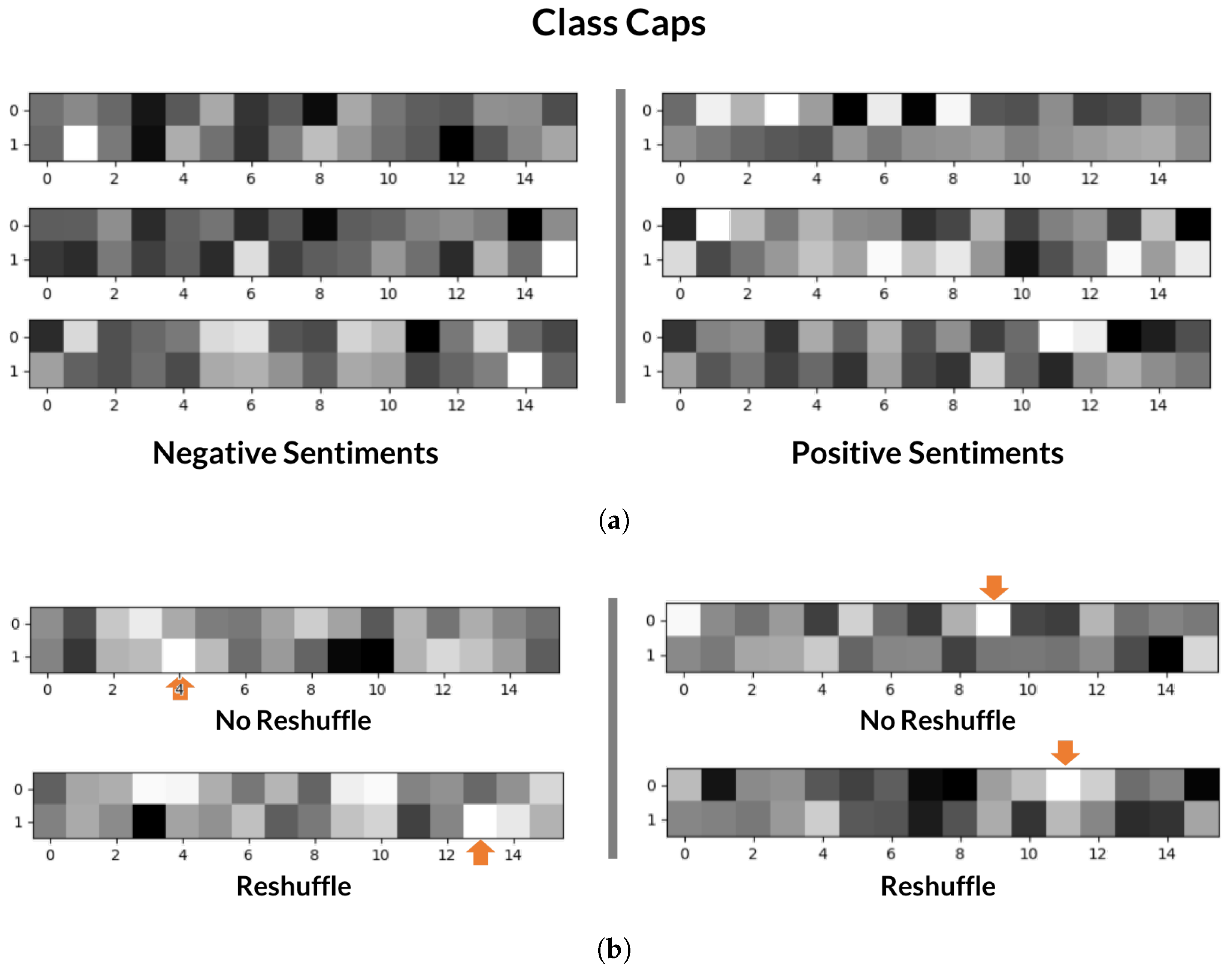
For a better understanding of what is happening inside the network, we visualized the output of the network on a number of internal layers. Looking into the Class Caps Layer, we found that the value of a certain capsule in a class is higher than all the other values if the input belongs to that class.
We present the output of the Class Caps Layer for three negative and three positive sentiments in
Figure 6a. Looking at
Figure 6a closely, we can observe that there is a pattern. For a negative sentiment, the brightest pixel, or the longest capsule in capsule notation, resides in the second row. For a positive sentiment, the brightest pixel is found in the first row. By looking at this figure, we can easily deduce that the longest capsule determines the class of our input data.
So as to examine how the change of sequential order of words affects the capsule information, we shuffled words in the input test data, keeping track of the location of strong words that are indicative of the polarity of the given test input. The outcomes of this experiment are given in
Figure 6b. As it can be seen from this figure, when shuffling words, the output of the Class Caps Layer also changes. Even though we can say that shuffling words results in change of the position of the longest capsule, we cannot clearly conclude which shuffled word caused which change.
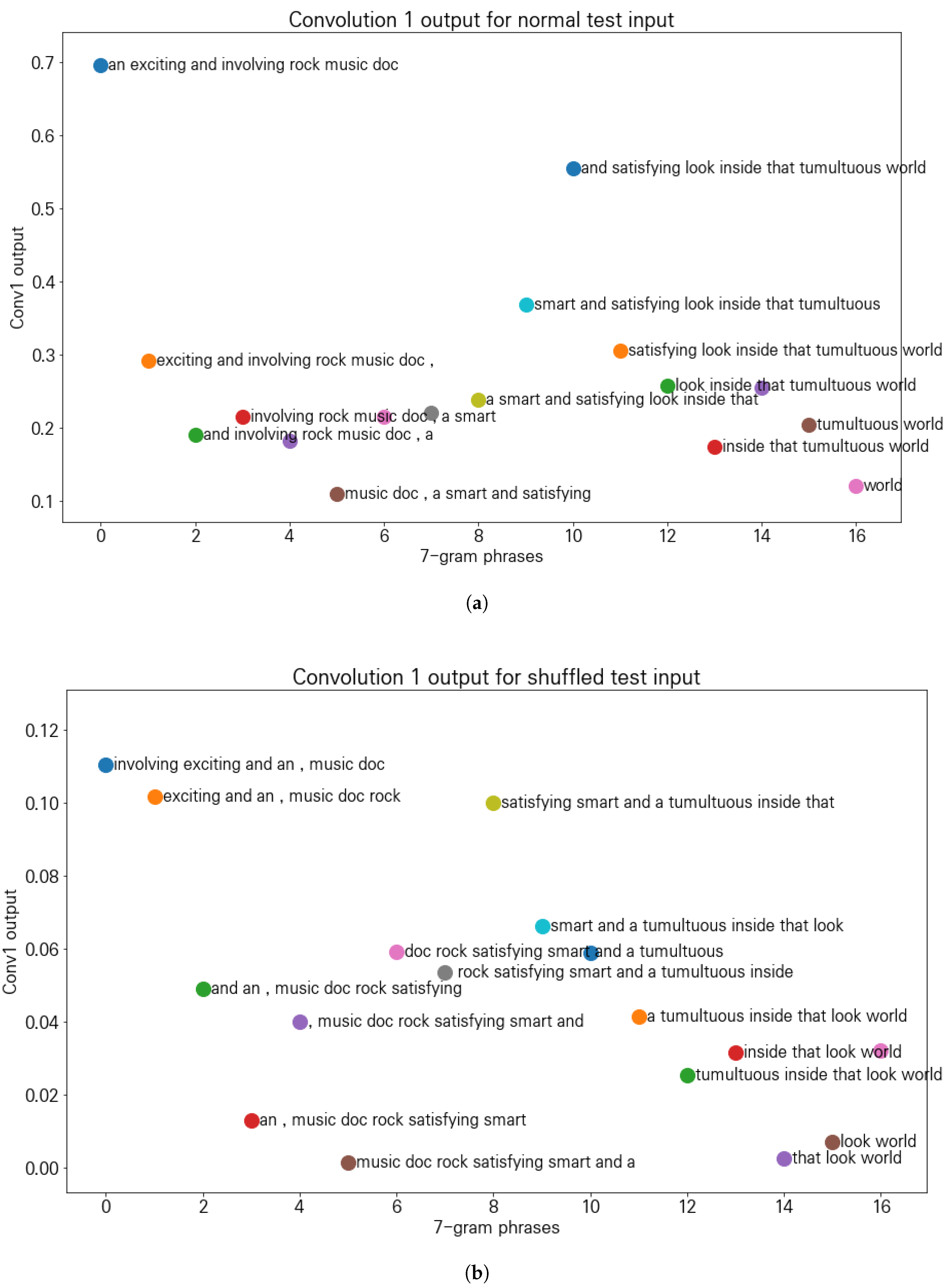
In order to further investigate how CapsNets handle spatial features of text at the phrase level, we did a visualization of the output at the first convolution layer with kernel size 7 and stride 1. By keeping the stride 1, a single output of this convolution layer maps to a single 7-gram phrase. To ensure that the CapsNet captures the order of words, we repeated the experiment by shuffling a given sentence in the test set, the results of which are given in
Figure 7. When given normal test input (see
Figure 7a, the CapsNet responds with a large output for 7-grams which contain higher polarity information than the other 7-grams. However, the outputs for the shuffled case usually have much lower values even for polarity indicating phrases and no significant difference in the output values among 7-gram phrases can be observed (see
Figure 7b. We performed several experiments with different shuffling and the outputs for those shuffled cases were almost similar to the one given in
Figure 7b. From this experiment, we argue that the CapsNet learns the spatial information presented in the input sentences.
4.6. Error Inspection
In this section, we present the number of sentences predicted correctly or incorrectly by different models and sample sentences with their predictions.
Table 5 shows the number of sentences that our CapsNet and the CNN models have classified correctly or incorrectly for the MR dataset. The results indicate that our CapsNet could classify some ambiguous sentences correctly which the CNN model failed to do. Out of 4265 test inputs, 3016 were classified correctly by both CapsNet and CNN models, and 308 sentences were classified incorrectly by both networks. Details are summarized in
Table 5.
In
Table 6, we present sample sentences classified correctly by CapsNet but incorrectly by the CNN model. Also presented is the prediction result for the LSTM model for ease of comparison.
The prediction confidence, or the maximum output value, is given with the predicted label for each model, where the true label is the same as the CapsNet’s prediction. For example, this sample sentence, “a painfully funny ode to bad behavior”, has more negative words and the CNN model was fooled to classify it as negative. However, the CapsNet was somehow able to classify it as positive sentiment probably by learning the phrase “painfully funny” is in fact a positive one. Another example, the sentence “a big, loud, bang the drum bore” might be ambiguous for learning as most of the words in the sentence happen to have a positive sentiment. As a whole, this sentence is labeled negative. While the CapsNet was able to label it negative, CNN failed to do so. The predictions by the LSTM model agree with those of the CapsNet except for one, which indicates that the CapsNet can serve as a good substitute of sequential models like LSTM for text classification tasks.
In
Table 7, we present sample sentences for which the CapsNet was not able to classify correctly but CNN did.
From these example sentences, we note that once in a while the CapsNet model may not be able to produce better performance than the CNN model for a short sentence like ‘a stuporously solemn film’. For sentences which lack polarity information or use ironic expressions like ‘there might be some sort of credible gender provoking philosophy submerged here, but who the hell cares?’, the CapsNet model will have difficulties in getting correct predictions as other models also will. Sometimes, reviewers may give a high score with a somewhat cynical sentence review like ‘though everything might be literate and smart, it never took off and always seemed static’ which will lead to incorrect labeling and hence incorrect prediction. Note that the LSTM model has shown the same wrong prediction as the CapsNet model on the above sentences. In the probability of prediction, however, the CapsNet model shows better potential than the LSTM model with lowered confidence scores in most of the sentences.
5. Conclusions
In this work, we presented an innovative CapsNet architecture for sentence classification. The performance of our model was compared with CNN and LSTM based models and other state-of-the-art models on five datasets. In most cases, our CapsNet model shows either superior or a very comparable performance to the other models, even with relatively simple network architecture. Just using the same dataset, our CapsNet model with a 2-phase training process was able to achieve the best results and hence we conclude that this multi-phase training approach can be very helpful to increase performance for networks with combined modules in any area of application. By intentionally changing the order of words in the test input, we learned that our CapsNet and the LSTM-based models are sensitive to the order of words in the given sentence while the CNN-based models were found to be less sensitive to the changes. This in turn means that CapsNet and LSTM based models can capture spatial information better than CNN-based models. This can be further interpreted as CapsNets can prevent adversarial attacks or can not be tricked by introducing artificial noise like intentional reshuffling. In addition to the numerical results in terms of accuracy, the results of visualization in the first convolution layer have further proven that the proposed CapsNet model learns the sequential order of words well.
In addition, we noticed from the experiments we performed that using pre-trained Word2vec models for encoding text data is of great importance. Apart from its use of word-to-vector encoding, the Word2vec embedding can also be used to generate synonym words for the purpose of data augmentation. Furthermore, due to the nature of the convolution operation used in CapsNet and CNN based models, the proposed network resulted in an increased processing speed compared to RNN-based models.
