Development of Rock Embedded Drilled Shaft Resistance Factors in Korea based on Field Tests

Abstract

Load and resistance factor design (LRFD) is a limit state design method that has been applied worldwide. Because the data for determining LRFD factors in Korea has been insufficient, the resistance factors suggested by American Association of State Highway and Transportation Officials (AASHTO) in the US have been used for design in Korea; however, these resistance factors were defined based on the characteristics of the predominant bedrock types in the U.S. As such, it remains necessary to determine resistance factors that reflect the bedrock conditions in Korea. Accordingly, in this study, LRFD resistance factors were determined using 13 sets of drilled shaft load test data. To obtain accurate resistance factors, calibration of the elastic modulus of the drilled shaft and the equivalent load–displacement curve considering the axial load and elastic settlement was conducted. After determining accurate resistance values, a reliability analysis was performed. The resistance factors were determined to be within 0.13–0.32 of the AASHTO factors for the shaft resistance, 0.19–0.29 for the base resistance, and 0.28–0.42 for the total resistance. This is equivalent to being 30–60% of the AASHTO-recommended values for the shaft resistance and 40–60% of the AASHTO-recommended values for the base resistance. These differences in resistance factors were entirely the result of discrepancies in the conditions of the rock in the US and Korea in which the shafts were founded.

1. Introduction

The load resistance factor design (LRFD) method can evaluate the resistance of a structure considering uncertainty based on the results of a reliability analysis. Using a reliability analysis, the probability of failure can be quantitatively evaluated, and the design of consistent and reliable geotechnical structures can be made possible. In recent decades, LRFD has replaced the allowable stress design (ASD) and working stress design (WSD) methods worldwide for the design of foundations [1,2]. The LRFD method was introduced in South Korea about a decade ago, and has been reflected in the design code for foundations in the country since 2012. The new Korean Highway Bridge Design Code (KHBDC) (limit state design) was published in 2012 and took effect for field applications starting in 2015. The resistance factors for foundations suggested by KHBDC [3], however, are based on American Association of State Highway and Transportation Officials (AASHTO) [4] in the U.S.; indeed, almost all the resistance factors were simply borrowed from AASHTO. Resistance factors for drilled shaft in rock from AASHTO were suggested as 0.50~0.55 for shaft resistance factors, and 0.50 for base resistances.

The resistance factors in AASHTO, however, reflect the characteristics of the bedrock found in the U.S., which may differ from the characteristics of the bedrock found in Korea. Notably, the resistance factors have already been calibrated for a number of states in U.S. based on area-specific bedrock types [5,6,7]. Also, the representative bedrock types in Korea are granite and gneiss classified as moderate or hard rock by strength criterion, they exhibit significant discontinuity and weathering. As such, these rocks are classified as weathered or soft rock by the weathering degree criterion [8]. This classification constitutes a discrepancy between the bedrock conditions in the U.S. and Korea, and as such, the direct application of the AASHTO resistance factors to Korean domestic design is inappropriate.

Considering these discrepancies, a great deal of research into resistance factors has been conducted in Korea. In 2008, the Korea Institute of Construction Technology [9] suggested total resistance factors for driven steel pipe piles (0.29~0.38 for target reliability index of 2.33) and drilled shafts (0.20~0.70 for target reliability index of 3.0). Jung [10] proposed total, shaft, and base resistance factors for drilled shafts using a numerical analysis. From Jung’s research, resistance factors for target reliability index of 3.0 were determined as 0.55~0.80 for total resistance, 0.20 for shaft resistance, and 0.20~0.70 for base resistance. Kim et al. [11] suggested the base and shaft resistance factors for axially loaded driven piles in sands based on the Imperial College pile (ICP) design method. The calculated resistance factors (target reliability index of 3.0) were 0.61~0.86 for base resistance and 0.55~0.96 for shaft resistance. Park [12,13] updated the total resistance factors for driven steel pipe piles based on Bayesian theory to incorporate the results of proof tests. The updated resistance factors were determined as 0.19~0.71 for target reliability index of 3.0. Recently, there were some researches to suggest the resistance factors for deep foundations using load test data in domestic region [14,15] and researches for suggestion of resistance factors and comparison according to design methods for shallow foundations [16,17].

Most of this previous research, however, has been limited to suggesting the total resistance factors, and the validity of the shaft and base resistance factors suggested by Jung are somewhat doubtful as they are derived from the results of a numerical analysis. Therefore, it remains necessary to determine accurate resistance factors for drilled shafts considering the discrepancy between the rock conditions in the U.S. and Korea using reliable load test results.

In this study, 13 sets of drilled shaft load test data obtained using strain gauges were collected and a load transfer analysis was conducted to determine accurate values for the shaft and base resistances. When the load tests were conducted as bi-directional load tests, the equivalent load–displacement curve was drawn to determine the total resistance. To obtain sufficiently accurate resistance values, calibrations of the elastic modulus of the concrete drilled shaft and of the equivalent load–displacement curve considering the axial load and elastic settlement were conducted. After determining accurate resistance values, a reliability analysis was performed to determine the target reliability index and resistance factors using the advanced first-order second-moment (AFOSM) reliability method.

2. Evaluation of Resistance for the Drilled Shaft

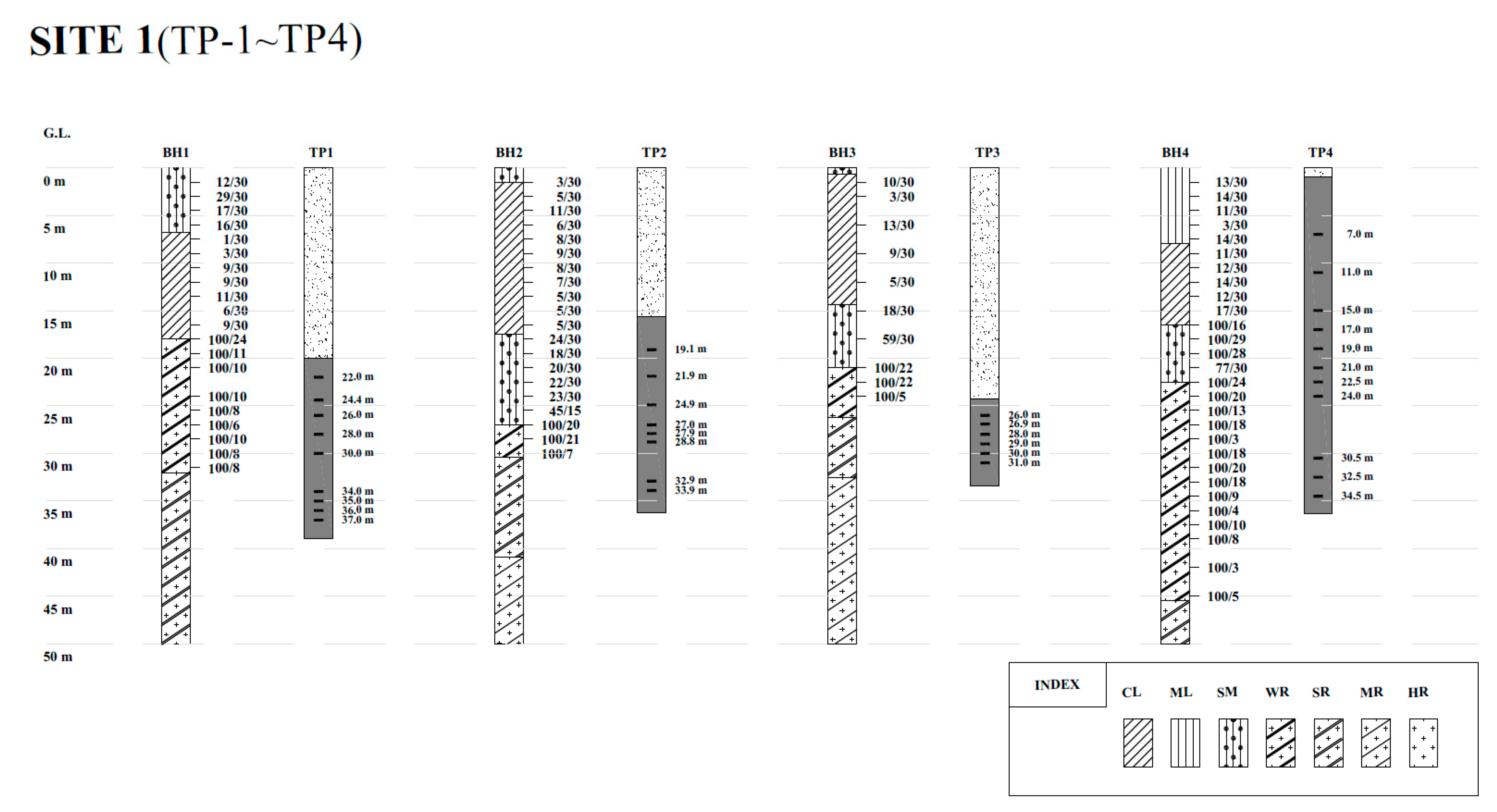
2.1. Collected Load Test Data

It is critical that accurate resistance values be determined. In the procedure for reliability-based resistance factor calibration, the measured resistance value can significantly influence the results of the reliability analysis and thus the subsequent the resistance factor calibration. Therefore, load test data obtained by strain gauges located in test drilled shafts were collected to provide accurate measurements of the shaft and base resistance. Based on these accurate shaft, base, and total resistance values obtained from the load transfer analysis, sufficiently accurate resistance factors can be determined.

In this study, a total of 13 sets of in-situ drilled shaft load test results were collected from three sites: shaft tests TP1–TP4 and TP5–TP8 were conducted on two different bridge construction sites and shaft tests TP9–TP13 were conducted on a building construction site (see Figure 1, Figure 2 and Figure 3 for site characteristics). Sites 1 and 2, corresponding to TP1–TP4 and TP5–TP8, respectively, contained large-diameter shafts, while Site 3 contained medium-diameter shafts. The drilled shaft profiles and rock properties, including the unconfined strength, RQD, and TCR were obtained from the site investigations, and data from the drilled shaft rock sockets were utilized to capture the conditions and effects of weathered, soft rock. Detailed information describing shaft construction and rock conditions can be found in

Table 1. Test shaft profile and site investigation results.

Shaft No.	Shaft Length (m)	Embedded Depth (m)	Shaft Diameter (m)	Construction Site	Rock Type	Weathering Degree*	Unconfined Strength (MPa)	RQD (%)	TCR (%)
TP 1	18.96	38.96	2.35	Site 1 (Bridge)	Gneiss & schist	Weathered and soft rock	3.1–19.8	0–13	54–100
TP 2	20.61	36.21	1.85			Weathered and soft rock	10.2–25.4	22–78	53–100
TP 3	9.11	33.41	1.35			Weathered and soft rock	5.6–25.0	25–72	80–100
TP 4	35.38	36.38	1.85			Weathered and soft rock	1.8–8.7	4–35	30–100
TP 5	40.14	55.42	3	Site 2 (Bridge)	Biotite granite	Weathered and soft rock	30.4–194	0–68	51–100
TP 6	44.10	56.60	2.4			Weathered rock	5–14	0–36	20–100
TP 7	45.10	51.20	2.4		Biotite granite & pegmatite	Weathered and soft rock	44–47	0–42	90–100
TP 8	40.01	52.26	2.4		Pegmatite, gneiss, & aplite	Weathered and soft rock	1–192	0–55	30–100
TP 9	14.0	14.0	1.5	Site 3 (Building)	Gneiss	Weathered rock	71.4–87.2	-	-
TP 10	13.5	13.5	1.0			Highly weathered rock	38	0	50
TP 11	13.5	13.5	1.0			Highly weathered rock	38	0	100
TP 12	13.5	13.5	1.0			Highly weathered rock	38	18–42	100
TP 13	13.5	13.5	1.0			Highly weathered rock	38	23–61	100

.

Over the last few decades, the bi-directional load test has been widely used to test drilled shafts due to its advantages compared to conventional top-down pile load tests. Among the load tests considered in this study, bi-directional load tests were used in Sites 1 and 2 in order to apply sufficient loading for the large-diameter drilled shafts. However, the shaft diameters in Site 3 were smaller, so bi-directional tests were not necessary to provide sufficient loading. Therefore, conventional pile (top-down) static loading tests were applied. The test programs are summarized in

Table 2. Test program.

Shaft No.	Loading Type	Load (MN)
TP 1	Bi-directional loading test	105.5
TP 2		49.1
TP 3		44.1
TP 4		36.8
TP 5		206.0
TP 6		166.8
TP 7		117.7
TP 8		88.3
TP 9	Top-down static loading test	19.1
TP 10		17.7
TP 11		17.7
TP 12		17.7
TP 13		17.7

.

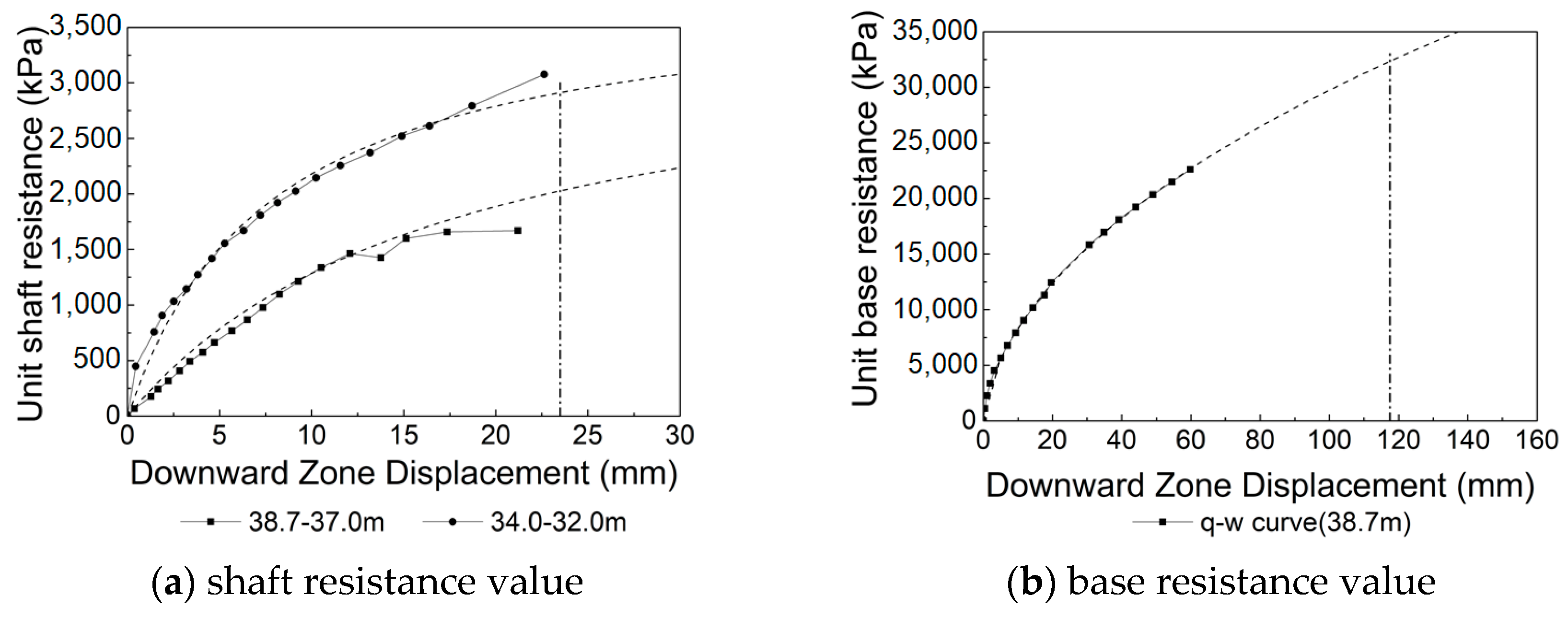
2.2. Procedures for Determination of Measured Resistance

Measured resistances were determined using the ultimate bearing capacities obtained from the load tests. In general cases, the measured resistance indicates the total measured resistance from the load-displacement curve of a static load test or the equivalent load–displacement curve of a bi-directional load test. However, load-displacement curves are generally drawn using the applied load and measured displacement of the shaft head, so they cannot include detailed ground properties or axial load transfer characteristics of a drilled shaft in the loading stage. To overcome these limitations and check the shaft and base resistances according to depth, a load transfer analysis using the measured strain data was performed.

The procedure for the calculation of measured resistance can be summarized as follows:

From the applied load and displacement measured during the load test, draw the load-displacement curve and determine the total resistance using this curve. If the load test was a bi-directional load test, draw the equivalent load-displacement curve

If it is necessary to calculate the shaft and base resistances, a load transfer analysis is conducted using data from strain gauges installed along the pile shaft that report the strain at each evaluated depth.

Calculate the axial load for each depth using a load transfer analysis as follows:

$$\mathrm{P}=\mathsf{\epsilon }\times \left({\mathrm{E}}_{\mathrm{pile}}\times {\mathrm{A}}_{\mathrm{pile}}\right)$$

(1)

where P is the calculated axial load at each depth, ε is measured strain at each depth, ${\mathrm{E}}_{\mathrm{pile}}$ is the elastic modulus of pile, and ${\mathrm{A}}_{\mathrm{pile}}$ is the area of the test shaft.

From the calculated axial load and displacement for each depth, draw the shaft resistance-displacement curve (f-w curve) and base resistance-displacement curve (q-w curve) and determine the shaft and base resistances using these curves.

2.3. Calibration for Load Test Transfer Analysis

The axial loads and the shaft and base resistance values can be determined by a load transfer analysis using strain data in conjunction with applied load levels. In a load transfer analysis, the elastic modulus of concrete is one of the most important parameters. Typically, a constant elastic modulus (${\mathrm{E}}_{50}$) has been applied in the past. However, the elastic modulus of concrete exhibits nonlinear stress-strain characteristics, and as such, nonlinearity should be considered in any load transfer analysis. According to Fellenius [18], the stress-strain relationship of a concrete pile shows nonlinear behavior when loaded, as can be seen in Figure 4. Therefore, the tangent modulus of the stress-strain relationship of a concrete pile is not constant but rather decreases with the downward slope of the curve with increasing strain.

In this study, the elastic modulus was calculated using the method of Fellenius, assuming the stress-strain relation of concrete to be a quadratic function. Then the calculated elastic modulus was applied to the load transfer analysis. For the calibration of the elastic modulus, the strain data near the load cell was used due to the large strain range present in the data. An example of the calibrated elastic modulus (TP 1) is shown in Figure 5. The solid line denotes the typically applied constant elastic modulus, while the dotted line describes the calibrated elastic modulus of the test drilled shaft.

After calibration, the elastic moduli of the shafts are applied to load transfer analyses, which were conducted using the measured strain data. First, the axial loads at each depth were determined using the data from the strain gauges as follows:

$$\mathrm{P}=\mathsf{\epsilon }\times \left({\mathrm{E}}_{\mathrm{Fellenius}}\times {\mathrm{A}}_{\mathrm{pile}}\right)$$

(2)

where P is the calculated axial load at each depth, ε is measured strain at each depth, ${\mathrm{E}}_{\mathrm{Fellenius}}$ is the calibrated elastic modulus, and ${\mathrm{A}}_{\mathrm{pile}}$ is the area of the test shaft. Using the calibrated load from Equation (2) for each depth, the load transfer analysis was performed to determine the measured shaft and base resistances.

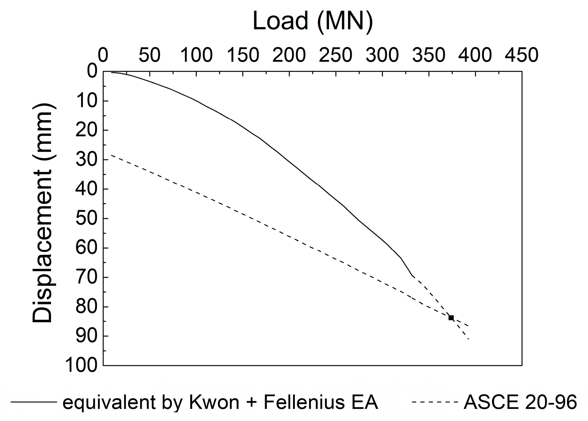
2.4. Calibration for the Equivalent Load-Displacement Curve

As described in the previous section, eight load tests were bi-directional and five were conventional. However, as the bi-directional drilled shaft load test relies upon a loading mechanism entirely different from that of the conventional pile load test, many investigators and practicing engineers have expressed concern that the bi-directional load test could produce inaccurate results, especially describing drilled shaft head settlement behavior. According to Kwon et al. [19], the top-down equivalent curve constructed from the bi-directional load test results predicted the drilled shaft head displacement to be about half that predicted by the conventional top-down load test. This is due to the difference in the load transferred to the soil layer. In the case of the bi-directional load test, the applied load is transferred to the rock layer, whose elastic modulus is larger than that of the soil layer, while in the case of the top-down load test, the load is transferred to the soil layer, which has a small elastic modulus and is much softer than the rock. The neglected elastic displacement is another reason for the potential inaccuracy of bi-directional load test results. In the procedure for obtaining the equivalent load-displacement curve, it is assumed that the drilled shaft is incompressible, so the elastic compression of the shaft is neglected during the construction of the equivalent load-displacement curve. As a result, many researchers including Yu et al. [20] have insisted that the additional elastic compression of the shaft be considered in a complete analysis. Accordingly, Kwon et al. suggested the use of the newly developed plotting method for the equivalent load-displacement curve considering the load transferred to the soil layer and the elastic compression.

To plot the equivalent load-displacement curves in this study, the axial load distributions were determined for each test drilled shaft and the load ratios quantifying the difference in load distribution between the top-down test and the bi-directional load test were calculated according to Kwon et al. The shaft displacement can be calculated from the end bearing load as follows:

$${\Delta \mathrm{w}}_{\mathrm{p}}=\frac{{\mathrm{Q}}_{\mathrm{pile}}{\mathrm{L}}_{\mathrm{pile}}}{{\mathrm{E}}_{\mathrm{pile}}{\mathrm{A}}_{\mathrm{pile}}}$$

(3)

where ${\mathrm{Q}}_{\mathrm{pile}}$ is the end bearing load for the downward movement of the pressure cell base w; ${\mathrm{A}}_{\mathrm{pile}}$ and ${\mathrm{L}}_{\mathrm{pile}}$ are the cross-sectional area and the length of the shaft, respectively; and ${\mathrm{E}}_{\mathrm{pile}}$ is the Young’s modulus of the shaft. Taking as many random points as required, the top-down equivalent curve can be constructed by connecting the points described by the calculated load-displacement coordinates. For example, in the case of shaft TP 2, the load ratio (=☐ABCEA/☐ABCDA) was approximately 3.82, indicating that the shaft head settlement should be w + 3.82Δ${\mathrm{w}}_{\mathrm{s}}$ to induce the downward movement of w at the shaft toe when the shaft is loaded from the top (Figure 6). The calculated calibrated elastic moduli and load ratios for all test cases are summarized in

Table 3. Summary of calibrated elastic modulus and load ratio.

Shaft No.	Calibrated Elastic Modulus for Load Test Transfer Analysis		Calibrated Load Ratio for the Equivalent Load-Displacement Curve
	${\mathbf{E}}_{50} \left(\mathbf{GPa}\right)$	${\mathbf{E}}_{\mathbf{Fellenius}} \left(\mathbf{GPa}\right)$	Load Ratio
TP1	32.29	32.91$-$0.0172$\mathsf{\mu }\mathsf{ϵ}$	1.00
TP2	34.67	29.19–0.0258$\mathsf{\mu }\mathsf{ϵ}$	3.82
TP3	37.97	35.71–0.0177$\mathsf{\mu }\mathsf{ϵ}$	1.00
TP4	37.74	37.78–0.0007$\mathsf{\mu }\mathsf{ϵ}$	1.00
TP5	33.13	41.26–0.0374$\mathsf{\mu }\mathsf{ϵ}$	4.44
TP6	39.72	35.66–0.0108$\mathsf{\mu }\mathsf{ϵ}$	4.31
TP7	38.15	40.81–0.0160$\mathsf{\mu }\mathsf{ϵ}$	1.22
TP8	36.39	42.02–0.0214$\mathsf{\mu }\mathsf{ϵ}$	1.42

.

Using the resulting axial load distribution and appropriately reduced elastic modulus, the equivalent load-displacement curves for each test shaft were constructed and compared with the results of the conventional load testing method. In this study, the equivalent load-displacement curves used by Kwon et al. and the calibrated elastic modulus used by Fellenius were selected to measure the resistance of the test drilled shafts. An example of the equivalent load-displacement curve is shown in Figure 7.

2.5. Measured Resistance from the Load Test Results

A load transfer analysis was conducted to measure the shaft and base resistance based on the drilled shaft load test results. The strain data were utilized to calculate the axial loads at each depth along the test shaft. In addition, the f-w curves, describing the unit shaft displacement for each depth, and the q-w curves, describing the unit displacement at the base of the drilled shafts, were established using the calculated axial loads. Then, according to O’Neill and Reese [21], the ultimate shaft and base resistance values were determined when the displacement of the shaft was equal to 1% and 5% of the shaft diameter, respectively. If the load tests were terminated before the applied loads reached these ultimate resistance values, the f-w and q-w curves were extrapolated using the hyperbolic method [22], as shown in Figure 8.

To determine the ultimate total resistance values, equivalent load-displacement curves were applied using the ASCE 20–96 method [23]. In this method, the ultimate total resistance is defined as the load at which the displacement of the shaft is equal to the elastic displacement + 3.81 + D/100 (mm). If a load test was terminated before the applied load reached this ultimate resistance value, the equivalent load-displacement curve was extrapolated using the hyperbolic method shown in Figure 9.

2.6. Predicted Resistance Values Obtained using Bearing Capacity Equations

Once the measured resistance values were obtained from the load test data, the predicted resistance values were used to evaluate the pile resistance uncertainty. While the measured resistance values were determined by analyzing the load test data, the predicted resistance values were calculated using bearing capacity equations. In this study, because the test piles were embedded in rock, the predicted resistance was calculated using a bearing capacity equation and the unconfined compressive strengths of the rock cores, as these values could be easily obtained through field and laboratory tests. Note that the selected bearing capacity equations are currently widely applied in actual design and specifications. The selected bearing capacity equations, required parameters, and remarks for the predicted shaft, base, and total resistance values are summarized in

Table 4. Bearing capacity equations for the predicted resistance.

(a) Shaft resistance.
Resistance component	Design method	Bearing capacity equation	Parameter
Shaft resistance	Carter & Kulhawy (1988)	${\mathrm{f}}_{\mathrm{s}}=6.47\sqrt{{\mathrm{q}}_{\mathrm{u}}}\left(\mathrm{kPa}\right)$	${\mathrm{q}}_{\mathrm{u}}$: Unconfined compressive strength of rock core (kPa)
	Horvath & Kenney (1979)	${\mathrm{f}}_{\mathrm{s}}=6.88\sqrt{{\mathrm{q}}_{\mathrm{u}}}\left(\mathrm{kPa}\right)$	${\mathrm{q}}_{\mathrm{u}}$: Unconfined compressive strength of rock core (kPa)
	FHWA (1999)	${\mathrm{f}}_{\mathrm{s}}=0.65\times {\mathrm{p}}_{\mathrm{a}}{\left[{\mathrm{q}}_{\mathrm{u}}/{\mathrm{p}}_{\mathrm{a}}\right]}^{0.5}\left(\mathrm{kPa}\right)$	${\mathrm{p}}_{\mathrm{a}}$: Atmospheric pressure = 101 kPa ${\mathrm{q}}_{\mathrm{u}}$: Unconfined compressive strength of rock core (kPa)
	Rowe & Armitage (1987)	${\mathrm{f}}_{\mathrm{s}}=14.89\sqrt{{\mathrm{q}}_{\mathrm{u}}}\left(\mathrm{kPa}\right)$	${\mathrm{q}}_{\mathrm{u}}$: Unconfined compressive strength of rock core (kPa)
(b) base resistance.
Resistance component	Design method	Bearing capacity equation	Parameter
Base resistance	Carter & Kulhawy (1988)	${\mathrm{q}}_{\mathrm{s}}=\left[{\mathrm{s}}^{0.5}+{\left(\mathrm{m}·{\mathrm{s}}^{0.5}+\mathrm{s}\right)}^{0.5}\right]{\mathrm{q}}_{\mathrm{u}}\left(\mathrm{kPa}\right)$	m,s: Mass properties ${\mathrm{q}}_{\mathrm{u}}$: Unconfined compressive strength of rock core (kPa)
	FHWA (1999)	${\mathrm{q}}_{\mathrm{s}}=3{\mathrm{K}}_{\mathrm{sp}}{\mathsf{\theta }\mathrm{q}}_{\mathrm{u}}\left(\mathrm{kPa}\right)$	${\mathrm{K}}_{\mathrm{sp}}$: Emperical factor θ: Depth factor ${\mathrm{q}}_{\mathrm{u}}$: Unconfined compressive strength of rock core (kPa)
	Zhang & Einstein (1998)	${\mathrm{q}}_{\mathrm{s}}=4.83{\sqrt{{\mathrm{q}}_{\mathrm{u}}}}^{0.51}\left(\mathrm{kPa}\right)$	${\mathrm{q}}_{\mathrm{u}}$: Unconfined compressive strength of rock core (kPa)
(c) total resistance.
Resistance component	Design method	Bearing capacity equation	Parameter
Total resistance	Carter & Kulhawy (1988)	${\mathrm{f}}_{\mathrm{s}}=6.47\sqrt{{\mathrm{q}}_{\mathrm{u}}}\left(\mathrm{kPa}\right)$	${\mathrm{q}}_{\mathrm{u}}$: Unconfined compressive strength of rock core (kPa)
		${\mathrm{q}}_{\mathrm{s}}=\left[{\mathrm{s}}^{0.5}+{\left(\mathrm{m}·{\mathrm{s}}^{0.5}+\mathrm{s}\right)}^{0.5}\right]{\mathrm{q}}_{\mathrm{u}}\left(\mathrm{kPa}\right)$	m,s: Mass properties ${\mathrm{q}}_{\mathrm{u}}$: Unconfined compressive strength of rock core (kPa)
	FHWA (1999)	${\mathrm{f}}_{\mathrm{s}}=0.65\times {\mathrm{p}}_{\mathrm{a}}{\left[{\mathrm{q}}_{\mathrm{u}}/{\mathrm{p}}_{\mathrm{a}}\right]}^{0.5}\left(\mathrm{kPa}\right)$	${\mathrm{p}}_{\mathrm{a}}$: Atmospheric pressure = 101 kPa ${\mathrm{q}}_{\mathrm{u}}$: Unconfined compressive strength of rock core (kPa)
		${\mathrm{q}}_{\mathrm{s}}=3{\mathrm{K}}_{\mathrm{sp}}{\mathsf{\theta }\mathrm{q}}_{\mathrm{u}}\left(\mathrm{kPa}\right)$	${\mathrm{K}}_{\mathrm{sp}}$: Emperical factor θ: Depth factor ${\mathrm{q}}_{\mathrm{u}}$: Unconfined compressive strength of rock core (kPa)

[24,25,26,27].

3. Determination of Resistance Factors

3.1. Determination of Statistical Parameters

3.1.1. Load Statistics

Contrary to the resistance statistics, it is known that regional variations in the load statistics are negligible. As a result, in this study, it was assumed that the load statistics in Korea are not significantly different from those in the U.S., meaning that the statistical load characteristics and load factors from the current AASHTO LRFD Specifications could be used. The dead and live load combination for the Strength I case was selected because this combination is considered the most conservative for the calibration of the resistance factors of axially loaded piles and drilled shafts, and is often the governing design load case in bridge design. The load factors and load statistical parameters for the Strength I case are summarized in

Table 5. Statistical characteristics of the loads.

$\mathbf{Load} \mathbf{Factor} \mathbf{of} \mathbf{Dead} \mathbf{Load} ({\mathbf{\gamma }}_{\mathbf{D}}=1.25)$		$\mathbf{Load} \mathbf{Factor} \mathbf{of} \mathbf{Live} \mathbf{Load} ({\mathbf{\gamma }}_{\mathbf{L}}=1.75)$
$\mathbf{Mean} \left({\mathbf{\lambda }}_{\mathbf{D}}\right)$	$\mathbf{Coefficient}\mathbf{of}\mathbf{Variation} \left(\mathbf{C}\mathbf{O}{\mathbf{V}}_{\mathbf{D}}\right)$	$\mathbf{Mean} \left({\mathbf{\lambda }}_{\mathbf{L}}\right)$	$\mathbf{Coefficient}\mathbf{of}\mathbf{Variation} \left(\mathbf{C}\mathbf{O}{\mathbf{V}}_{\mathbf{L}}\right)$
1.05	0.10	1.15	0.20

.

3.1.2. Resistance Statistics

The uncertainty of the ground conditions, design parameters, bearing capacity equations, and the drilled shaft resistance is established using a bias factor. The statistical characteristics of resistance are represented in terms of this bias factor, which is defined as the ratio of the measured resistance to the predicted resistance. The measured and predicted resistances were determined from the load test and bearing capacity equations as mentioned in previous sections. In this study, 13 load test cases were collected and used. These load tests were planned to install the strain gauge by depth and perform the load transfer analysis. From load transfer analysis, shaft and base resistances were separately determined and summarized as measured resistances in

Table 6. Calculated bias factors for shaft resistance.

Shaft No.	Depth (m)	Measured Shaft Resistance (MPa)	Carter & Kulhawy (1988)		Horvath & Kenney (1979)		FHWA (1999)		Rowe & Armitage (1987)
			Predicted Resistance (MPa)	Bias Factor	Predicted Resistance (MPa)	Bias Factor	Predicted Resistance (MPa)	Bias Factor	Predicted Resistance (MPa)	Bias Factor
TP1	35.0–36.0	1.22	0.36	1.53	0.38	1.44	0.36	1.51	0.83	0.66
	36.0–37.0	2.45	0.80	3.18	0.85	2.99	0.81	3.15	1.84	1.38
	37.0–38.7	1.90	0.77	2.09	0.82	1.96	0.78	2.07	1.77	0.91
TP2	28.8–32.9	0.81	0.89	0.9	0.95	0.85	0.90	0.89	2.06	0.39
	32.9–33.9	0.89	0.77	1.16	0.82	1.09	0.78	1.14	1.77	0.5
	33.9–35.3	2.06	1.03	2	1.10	1.88	1.04	1.98	2.37	0.87
TP3	26.9–28.0	0.68	0.57	1.19	0.61	1.12	0.58	1.18	1.32	0.52
	28.0–29.0	0.37	0.65	0.57	0.69	0.54	0.66	0.56	1.50	0.25
	29.0–30.0	1.40	0.82	1.7	0.88	1.6	0.83	1.69	1.90	0.74
	30.0–31.0	1.79	0.81	2.21	0.86	2.08	0.82	2.19	1.86	0.96
	31.0–33.1	2.69	0.67	4.02	0.71	3.78	0.68	3.98	1.54	1.74
TP4	24.0–30.5	0.24	0.27	0.87	0.29	0.82	0.28	0.86	0.63	0.38
TP5	44.0–46.5	0.32	2.18	0.15	2.32	0.14	2.20	0.15	5.01	0.06
	46.5–48.5	2.85	2.58	1.1	2.75	1.04	2.61	1.09	5.95	0.48
	48.5–50.5	2.00	2.85	0.7	3.03	0.66	2.88	0.69	6.56	0.3
	50.5–52.5	1.44	2.67	0.54	2.84	0.51	2.69	0.54	6.14	0.23
	52.5–54.5	1.52	1.26	1.2	1.34	1.13	1.27	1.19	2.90	0.52
TP7	45.5–50.21	3.35	1.36	2.46	1.45	2.31	1.37	2.44	3.13	1.07
TP8	46.26–48.26	1.22	0.28	4.36	0.30	4.1	0.28	4.32	0.64	1.89
	48.26–49.76	1.17	0.38	3.04	0.41	2.85	0.39	3.01	0.88	1.32
	49.76–51.35	1.60	0.55	2.9	0.59	2.73	0.56	2.87	1.27	1.26

,

Table 7. Calculated bias factors for base resistance.

Shaft No.	Depth (m)	Measured Base Resistance (MPa)	Carter & Kulhawy (1988)		FHWA (1999)		Zhang & Einstein (1999)
			Predicted Resistance (MPa)	Bias Factor	Predicted Resistance (MPa)	Bias Factor	Predicted Resistance (MPa)	Bias Factor
TP 1	38.96	32.33	11.76	2.75	12.71	2.54	21.91	1.48
TP 2	36.21	40.43	10.64	3.80	18.92	2.14	26.42	1.53
TP 3	33.41	46.68	61.92	0.75	93.65	0.50	31.70	1.47
TP 5	55.42	55.73	105.72	0.53	151.32	0.37	49.83	1.12
TP 7	51.2	35.01	14.15	2.48	34.17	1.02	34.42	1.02
TP 8	52.26	23.94	26.30	0.91	19.94	1.20	31.12	0.77
TP 10	13.5	10.13	9.49	1.07	20.52	0.49	30.88	0.33
TP 11	13.5	14.75	9.49	1.55	21.43	0.69	30.88	0.48
TP 12	13.5	32.94	26.50	1.24	20.52	1.61	30.88	1.07
TP 13	13.5	13.24	33.49	0.40	20.52	0.65	30.88	0.43

and

Table 8. Calculated bias factors for total resistance.

Shaft No.	Depth (m)	Measured Total Resistance (MN)	Carter & Kulhawy (1988)		FHWA (1999)
			Predicted Resistance (MN)	Bias Factor	Predicted Resistance (MN)	Bias Factor
TP 1	38.96	373.86	83.60	4.47	88.07	4.25
TP 2	36.21	144.85	64.49	2.25	87.09	1.66
TP 3	33.41	151.50	107.23	1.41	152.83	0.99
TP 5	55.42	335.88	854.78	0.39	1147.41	0.29
TP 7	51.2	356.00	101.48	3.51	181.52	1.96
TP 8	52.26	200.61	118.79	1.69	93.65	2.14

. However, due to some reasons like site condition, pile construction quality and proficiency of engineer, load transfer analysis was not able to perform in some cases especially Site 3(TP 9~TP 13). The strain gauge condition of test piles in Site 3(TP 9~TP 13) were not good to measure the strain and perform the load transfer analysis, it was impossible to determine the shaft resistances. So, only base resistances for TP 9~TP13 were used for this study. Consequently, 21 bias factors for shaft resistance, 10 for base resistance, and 6 for total resistance were calculated and are summarized in Table 6, Table 7 and Table 8.

These calculated bias factors were then used to determine the resistance statistics, such as the mean, standard deviation, and coefficient of variation. These resistance statistics are summarized in

Table 9. Statistical characteristics of shaft resistance

(a) Shaft resistance.
Design method	Pile no.	Mean (${\lambda }_R$)	Standard deviation	Coefficient of variation
Carter & Kulhawy (1988)	21	1.80	1.17	0.65
Horvath & Kenney (1979)	21	1.70	1.10	0.65
FHWA (1999)	21	1.79	1.16	0.65
Rowe & Armitage (1987)	21	0.78	0.51	0.65
(b) Base resistance.
Design method	Pile no.	Mean ( ${\lambda }_R$)	Standard deviation	Coefficient of variation
Carter & Kulhawy (1988)	9	1.30	0.83	0.64
FHWA (1999)	10	1.12	0.75	0.67
Zhang & Einstein (1998)	10	0.97	0.45	0.47
(c) Total resistance.
Design method	Pile no.	Mean ( ${\lambda }_R$)	Standard deviation	Coefficient of variation
Carter & Kulhawy (1988)	6	2.29	1.48	0.65
FHWA (1999)	6	1.88	1.34	0.71

. In this procedure, extremely outlying data points may not be representative of the resistance due to some large error; therefore, the bias factor values outside the boundary defined by the mean plus two times the standard deviation were omitted according to Paikowsky [28]. In case of Carter & Kulhawy, statistics based on all data were calculated as follows; mean as 1.55, Standard deviation as 1.11, and COV as 0.72. However, boundary of bias factors was calculated as 3.77 (mean plus times of standard deviation), so outlying data (bias factor of TP 2 as 3.80 in Table 7) was omitted for statistical analysis. Consequently, statistics were calculated based on nine data (excluding TP 2), and results were summarized in Table 9.

3.2. Determination of Target Reliability Index

To consider the transition from ASD to LRFD, a reliability analysis was performed and the reliability indices of shafts designed using the current design practice (ASD) were estimated. The Korean design standard for foundation structures requires a safety factor of 3.0 for pile bearing capacity design; therefore, the reliability analysis was performed for safety factors of 2.0–5.0 using the advanced first-order second moment (AFOSM) method.

The AFOSM method, named so because it is based on a first-order Taylor series approximation of the limit state function and because it uses only the second-moment statistics (mean and COV) of the variables, was proposed by Hasofer and Lind [29] and is known as one of the most accurate methods of reliability analysis. When the AFOSM method is used, the limit state function is linearized at the design point on the nonlinear failure surface, so the full distribution of information can be used rather than simply the mean value of the random variables. The results of the AFOSM reliability analysis are summarized in

Table 10. Reliability analysis results.

(a) Shaft resistance.
Bearing capacity equation	Reliability index (${\beta }_T$)
	FS = 2.0	FS = 3.0	FS = 4.0	FS = 5.0
Carter & Kulhawy (1988)	1.73	2.40	2.88	3.25
Horvath & Kenney (1979)	1.62	2.30	2.78	3.15
FHWA (1999)	1.71	2.39	2.87	3.24
Rowe & Armitage (1987)	0.34	1.01	1.49	1.86
(b) Base resistance.
Bearing capacity equation	Reliability index (${\beta }_T$)
	FS = 2.0	FS = 3.0	FS = 4.0	FS = 5.0
Carter & Kulhawy (1988)	1.20	1.89	2.37	2.75
FHWA (1999)	0.89	1.41	2.02	2.38
Zhang & Einstein (1998)	1.08	1.97	2.60	3.08
(c) Total resistance.
Bearing capacity equation	Reliability index (${\beta }_T$)
	FS = 2.0	FS = 3.0	FS = 4.0	FS = 5.0
Carter & Kulhawy (1988)	2.12	2.80	3.26	3.65
FHWA (1999)	1.61	2.24	2.68	3.03

.

Recently, AASHTO LRFD [1] selected a target reliability index of 3.0 for a typical drilled shaft. Moreover, KICT [5] suggested a target reliability index between 3.0–3.5 for drilled shafts. Based on the reliability analysis results and previous research [1,5], target reliability indices (${\mathsf{\beta }}_{\mathrm{T}}$) of 2.5, 3.0, and 3.5 were selected for the calibration of the resistance factors in this study.

3.3. Determination of Resistance Factors

Considering three different target reliability indices (${\mathsf{\beta }}_{\mathrm{T}}$ = 2.5, 3.0, and 3.5), the resistance factors were calibrated using the AFOSM method. The calibration results were expressed as the relationship between the reliability index and the resistance factor. The results are shown in Figure 10, and the resistance factors for each bearing capacity equation and target reliability index are summarized in

Table 11. Results for the resistance factors.

(a) Shaft resistance.
Bearing capacity equation	Resistance factor			Note
	${\beta }_T$= 2.5	${\beta }_T$= 3.0	${\beta }_T$= 3.5	AASHTO (2015) ${\beta }_T$= 3.0
Carter & Kulhawy (1988)	0.45	0.32	0.24	0.5
Horvath & Kenney (1979)	0.42	0.30	0.22	0.55
FHWA (1999)	0.44	0.32	0.24	0.55
Rowe & Armitage (1987)	0.19	0.13	0.11	-
(b) Base resistance.
Bearing capacity equation	Resistance factor			Note
	${\beta }_T$= 2.5	${\beta }_T$= 3.0	${\beta }_T$= 3.5	AASHTO (2015) ${\beta }_T$= 3.0
Carter & Kulhawy (1988)	0.32	0.24	0.21	0.5
FHWA (1999)	0.25	0.19	0.17	0.5
Zhang & Einstein (1998)	0.37	0.29	0.24	-
(c) Total resistance.
Bearing capacity equation	Resistance factor			Note
	${\beta }_T$= 2.5	${\beta }_T$= 3.0	${\beta }_T$= 3.5	AASHTO (2015) ${\beta }_T$= 3.0
Carter & Kulhawy (1988)	0.57	0.42	0.30	-
FHWA (1999)	0.40	0.28	0.22	-

.

The resistance factors were determined for the target reliability indices of 2.5, 3.0, and 3.5 and compared with the resistance factors suggested by AASHTO. For the AASHTO-recommended reliability index of 3.0, the shaft resistance factors are within 0.13–0.32 of the AASHTO-based values, and the base resistance factors are within 0.19–0.29 of the AASHTO-based values each bearing capacity equation. These resistance factors are 30–60% of the AASHTO-recommended values for the shaft resistance and 40–60% of the AASHTO-recommended values for the base resistance.

These differences in resistance factors are the result of the discrepancy in the conditions of the rocks in which the drilled shafts are founded. The resistance factors suggested by AASHTO are determined based on sedimentary and intact rock conditions, while according to geologic maps from Korea Structure and Foundation Structure Design Specifications [30], the representative types of bedrock in Korea are granite and gneiss, classified as weathered or soft rock by the weathering degree criterion. Clearly, this difference in rock condition has a clear and detrimental effect on drilled shaft performance that must be appropriately accounted for in the LRFD design resistance factors used in Korea. Also, suggested resistance factors were based on only 13 load test cases considering regional characteristics in Korea. But, if additional load test data will be collected, LRFD methods can be updated and calibrated the resistance factors based on reliability analysis. So, results in this study are expected to be helpful for future reference.

4. Conclusions

The load resistance factor design (LRFD) method can be used evaluate the resistance of a structure considering uncertainty based on a reliability analysis. In recent decades, LRFD has replaced allowable stress design (ASD) and working stress design (WSD) for the design of foundations worldwide, and is reflected in the design code for foundations in South Korea. However, the resistance factors used in Korea are based on those recommended by AASHTO in the U.S., which reflect characteristics of the bedrock in the U.S. that may differ from those of the bedrock in Korea. Based on such discrepancies in rock conditions, the direct application of the AASHTO-recommended resistance factors for design in Korea is inappropriate. Therefore, it was necessary to determine accurate resistance factors for drilled shafts considering the rock conditions in Korea based on reliable load test results.

In this study, 13 sets of drilled shaft load test data were obtained using strain gauges, and a load transfer analysis was performed to determine the accurate shaft and base resistance values. For bi-directional load tests, the equivalent load-displacement curve was drawn to determine the total resistance. Calibrations of the elastic modulus of the drilled shaft concrete and of the equivalent load-displacement curve considering the axial load and elastic settlement were conducted to obtain more accurate resistance values. After determining accurate resistance values, a reliability analysis was performed to determine the target reliability index and the resistance factors using the advanced first-order second-moment (AFOSM) reliability method.

For the AASHTO-recommended target reliability index of 3.0, the shaft resistance factors were found to be within 0.13–0.32 of the AASHTO-based values, the base resistance factors were within 0.19–0.29 of the AASHTO-based values, and the total resistance factors were within 0.28–0.42 of the AASHTO-based values for each bearing capacity equation evaluated. The resistance factors were accordingly determined to be 30–60% of the AASHTO-recommended values for the shaft resistance and 40–60% of the AASHTO-recommended values for the base resistance. These differences in resistance factors are the result of discrepancies in the condition of the rocks in which the drilled shafts were founded. The resistance factors suggested by AASHTO are determined using sedimentary and intact rock conditions prevalent in the US, while the bedrock in Korea tends to be weathered or soft granite and gneiss. This study has thus determined adjusted resistance factors to account for this difference in rock type and condition, providing improved design safety and load resistance accuracy when using drilled shafts in Korea. Also, suggested resistance factors were based on only 13 load test cases considering the regional characteristics in Korea. But, if additional load test data is collected, LRFD methods can update and calibrate the resistance factors based on reliability analysis. So, the results in this study are expected to be helpful for future reference.

References

1. Abu-Farsakh, M.Y.; Yu, X.; Zhang, Z. Calibration of side, tip, and total resistance factors for load and resistance factor design of drilled shafts. Transp. Res. Rec. J. Transp. Res. Board 2012, 2310, 38–48. [Google Scholar] [CrossRef]
2. Basu, D.; Salgado, R. Load and resistance factor design of drilled shafts in sand. J. Geotech. Geoenviron. Eng. 2012, 138, 1455–1469. [Google Scholar] [CrossRef]
3. Ministry of Construction and Transportation. Korea Highway Bridge Design Code (Limit State Design); Korea Road and Transportation Association: Seoul, Korea, 2012. (In Korean) [Google Scholar]
4. AASHTO. AASHTO LRFD Bridge Design Specifications, 6th ed.; AASHTO: Washington, DC, USA, 2015. [Google Scholar]
5. Long, J.; Hendrix, J.; Baratta, A. Evaluation/Modification of IDOT Foundation Piling Design and Construction Policy; Rep. No. ICT-09-037; Illinois Center for Transportation: Rantoul, IL, USA, 2009. [Google Scholar]
6. Garder, J.A.; Ng, K.W.; Sritharan, S.; Roling, M.J. Development of a Database for Drilled SHAft Foundation Testing (DSHAFT); Rep. No. InTrans 10-366; Institute for Transportation, Iowa State University: Ames, IA, USA, 2012. [Google Scholar]
7. Stanton, K.; Motamed, R.; Elfass, S. Robust LRFD resistance factor calibration for axially loaded drilled shafts in Las Vegas. J. Geotech. Geoenviron. Eng. 2017, 143, 06017004. [Google Scholar] [CrossRef]
8. Kim, S.J.; Kwon, O.S.; Jung, S.J.; Han, J.T.; Kim, M.M. Determination of Resistance Factors of Load and Resistance Factor Design for Drilled Shaft Based on Load Test. J. Korean Geotech. Soc. 2010, 26, 17–24. [Google Scholar]
9. Korea Institute of Construction Technology (KICT). Determination of Resistance Factors for Foundation Structure Design by LRFD; Research Policy/Infrastructure Development Program, Ministry of Land, Transport and Maritime Affairs: Seoul, Korea, 2008. [Google Scholar]
10. Jung, S.J. Calibration of Resistance Factors of Load and Resistance Factor Design for Drilled Shafts Embedded in Weathered Rock. Ph.D. Thesis, Seoul National University, Seoul, Korea, 2010. [Google Scholar]
11. Kim, D.W.; Chung, M.K.; Kwak, K.S. Resistance factor calculations for LRFD of axially loaded driven piles in sands. KSCE J. Civ. Eng. 2011, 15, 1185–1196. [Google Scholar] [CrossRef]
12. Park, J.H. Resistance Factor Calibration and Bayesian Implementation for LRFD of Axially-Loaded Driven Steel Pipe Piles. Ph. D. Thesis, Seoul National University, Seoul, Korea, 2011. [Google Scholar]
13. Park, J.H.; Huh, J.W.; Kim, K.J.; Chung, M.K.; Lee, J.H.; Kim, D.W.; Kwak, K.S. Resistance Factors Calibration and Its Application using Static Load Test Data for Driven Steel Pipe Piles. KSCE J. Civ. Eng. 2013, 17, 929–938. [Google Scholar] [CrossRef]
14. Kim, H.T.; Kim, D.H.; Lim, J.C.; Park, K.H.; Lee, I.H. Resistance Factor and Target Reliability Index Calculation of Static Design Methods for Driven Steel Pipe Pile in Gwangyang. J. Korea Acad.-Ind. Coop. Soc. 2015, 16, 8128–8139. [Google Scholar]
15. Park, J.B.; Kwon, Y.H. Estimation of Resistance Coefficient of PHC Bored Pile by Load Test. LHI J. 2017, 8, 233–247. [Google Scholar]
16. Kim, D.G.; Kim, H.T.; Suh, J.W.; Yoo, N.J. Analysis of LRFD Resistance Factor for Shallow Foundation on Weathered Soil Ground. J. Korean Geo-Environ. Soc. 2015, 16, 5–11. [Google Scholar] [Green Version]
17. Kim, D.G.; Hwang, H.S.; Yoo, N.J. Comparison of Safety Margin of Shallow Foundation on Weathered Soil Layer According to Design Methods. J. Korean Geo-Environ. Soc. 2016, 17, 55–64. [Google Scholar] [CrossRef] [Green Version]
18. Fellenius, B.H. Tangent modulus of piles determined from strain data. In Proceedings of the ASCE Geotechnical Engineering Division Foundation Congress, Evanston, IL, USA, 25–29 June 1989; pp. 500–510. [Google Scholar]
19. Kwon, O.S.; Choi, Y.K.; Kwon, O.K.; Kim, M.M. Method of Estimating Pile Load-displacement Curve Using Bi-directional Load Test. J. Korean Geotech. Soc. 2006, 22, 11–19. [Google Scholar]
20. Yu, X.; Abu-Farsakh, M.Y.; Yoon, S.M.; Tsai, C.; Zhang, Z. Implementation of LRFD of drilled shafts in Louisiana. J. Infrastruct. Syst. 2011, 18, 103–112. [Google Scholar] [CrossRef]
21. O’Neill, M.W.; Reese, L.C. Drilled Shafts: Construction Procedures and Design Methods; FHWA-IF-99-025; FHWA: Washington, DC, USA, 1999.
22. Gupta, R.C. Hyperbolic Model for Load Tests on Instrumented Drilled Shafts in Intermediate Geomaterials and Rock. J. Geotech. Geoenviron. Eng. 2012, 138, 1407–1414. [Google Scholar] [CrossRef]
23. ASCE. Standard Guidelines for the Design and Installation of Pile Foundations; ASCE 20-96; ASCE: Reston, VA, USA, 1997. [Google Scholar]
24. Carter, J.P.; Kulhawy, F.H. Analysis and Design of Drilled Shaft Foundations Socketed into Rock; Report EL-5918; Electric Power Research Institute: Palo Alto, CA, USA, 1988. [Google Scholar]
25. Horvath, R.G.; Kenney, T.C. Shaft resistance of rock-socketed drilled piers. In Symposium on Deep Foundations; ASCE: Atlanta, GA, USA, 25 October 1979; pp. 182–214. [Google Scholar]
26. Rowe, R.K.; Armitage, H.H. A design method for drilled piers in soft rock. Can. Geotech. J. 1987, 24, 126–142. [Google Scholar] [CrossRef] [Green Version]
27. Zhang, L.; Einstein, H.H. End bearing capacity of drilled shafts in rock. J. Geotech. Geoenviron. Eng. 1998, 124, 574–584. [Google Scholar] [CrossRef]
28. Paikowsky, S.G. Load and Resistance Factor Design (LRFD) for Deep Foundations; NCHRP Report 24-17; Transportation Research Board: Washington, DC, USA, 2004. [Google Scholar]
29. Hasofer, A.M.; Lind, N.C. Exact and invariant second moment code format. J. Eng. Mech. Divis. 1974, 100, 111–121. [Google Scholar]
30. Ministry of Land, Transport and Maritime Affairs. Korea Structure and Foundation Structure Design Specification; Korean Geotechnical Society: Seoul, Korea, 2003. (In Korean) [Google Scholar]
Figure 1. Site investigation results (Site 1).
Applsci 09 02201 g001
Figure 2. Site investigation results (Site 2).
Applsci 09 02201 g002
Figure 3. Site investigation results (Site 3).
Applsci 09 02201 g003
Figure 4. Typical data of static loading test on a concrete pile
Applsci 09 02201 g004
Figure 5. Calibrated elastic modulus of TP 1.
Applsci 09 02201 g005
Figure 6. Estimation of the top-down load distribution from the bi-directional load test (TP 2).
Applsci 09 02201 g006
Figure 7. Equivalent load-displacement curve of TP 2.
Applsci 09 02201 g007
Figure 8. Determination of the ultimate shaft and base resistance values for TP 1.
Applsci 09 02201 g008
Figure 9. Determination of the ultimate total resistance value at TP 1.
Applsci 09 02201 g009
Figure 10. Relationship between the reliability index and the resistance factors for each component.
Applsci 09 02201 g010