Article

Confidence Measures for Deep Learning in Domain Adaptation

1
Department of Information Engineering and Mathematics, University of Siena, 53100 Siena, Italy
2
Department of Computer Science, University of Copenhagen, 2100 Copenhagen, Denmark
3
Cerebriu A/S, 2100 Copenhagen, Denmark
*
Author to whom correspondence should be addressed.
Appl. Sci. 2019, 9(11), 2192; https://doi.org/10.3390/app9112192
Submission received: 18 April 2019 / Revised: 16 May 2019 / Accepted: 23 May 2019 / Published: 29 May 2019
(This article belongs to the Special Issue Advances in Deep Learning)

Abstract

:
In recent years, Deep Neural Networks (DNNs) have led to impressive results in a wide variety of machine learning tasks, typically relying on the existence of a huge amount of supervised data. However, in many applications (e.g., bio–medical image analysis), gathering large sets of labeled data can be very difficult and costly. Unsupervised domain adaptation exploits data from a source domain, where annotations are available, to train a model able to generalize also to a target domain, where labels are unavailable. Recent research has shown that Generative Adversarial Networks (GANs) can be successfully employed for domain adaptation, although deciding when to stop learning is a major concern for GANs. In this work, we propose some confidence measures that can be used to early stop the GAN training, also showing how such measures can be employed to predict the reliability of the network output. The effectiveness of the proposed approach has been tested in two domain adaptation tasks, with very promising results.

1. Introduction

Recently, deep learning has pushed the state of the art in several visual recognition tasks, e.g., in object detection [1], semantic segmentation [2,3], speech recognition [4], and medical image analysis [5,6]. All of these results rely on the availability of large datasets of annotated images (e.g., ImageNet [7]). However, due to domain shift [8], models trained on these datasets do not generalize well to different sets of data [9,10]. Usually, to be adapted to a new domain, the model should be fine-tuned; unfortunately, it is often difficult to obtain enough labeled data. Unsupervised domain adaptation [11] is used when the supervision is available for the source but not for the target domain. It aims at building a model on the source dataset that correctly generalizes also on target samples, despite the domain shift. In particular, domain adaptation can be seen as a particular case of transfer learning that leverages labeled data of a source domain, to learn a classifier that can be applied on a target domain, in which supervised data are not available. In general, it is assumed that the two domains share the same class and that the target domain is related, but not identical, to the source domain. In this framework, Generative Adversarial Networks (GANs) [12] have been successfully employed [13], due to their ability to reproduce data distributions. Indeed, GANs are based on two competing networks, called the generator and the discriminator, being the last engaged in determining whether a sample is produced by the generator or it belongs to the original data distribution. In unsupervised domain adaptation, the adversarial training has been employed to induce the model to learn the same distribution for the source and the target domain, this is done at image or feature level. Three main problems are often encountered with this approach. The first issue is directly related to the very nature of GANs, for which deciding when the training should be stopped is generally a difficult task. In fact, usually, when convergence is not achieved, a visual evaluation of the generated images is used to stop the learning, an almost heuristic approach, difficult to be standardized. Another limit is directly related to the absence of labeled samples in the target domain, which makes it impossible to evaluate the network performance with the usual method based on a validation set. Finally, the last problem is related to the reliability of the model output, particularly impactful when the input is significantly different from the training patterns. If, in general, this is a limit common to all neural networks, it has a particular relevance in domain adaptation due to the different data distribution of the source and target datasets.
In this research, we studied several confidence measures, not depending on data labels, that allow evaluating the reliability of the network outputs, mitigating all the above-mentioned problems. The proposed measures are related to the two major sources of uncertainty that a model may have [14]:
  • Epistemic uncertainty is related to the lack of knowledge and, in the case of a neural network model, means that the parameters are poorly determined due to the data scarcity, so that the posterior probability over them is broadly captured.
  • Aleatoric uncertainty is due to genuine stochasticity in the data; if the data are inherently noisy, then also the best prediction may have a high entropy.
The experiments were carried out using a recently proposed domain adaptation method [13] that employs GANs to learn feature distributions indistinguishable from the source and the target domain. The employed confidence measures were firstly applied in two unsupervised domain adaptation tasks: SVHN [15] → MNIST [16] and CIFAR [17]→ STL [18]. The experimental results show that, based on the confidence measures, the domain adaptation process can be stopped close to the optimum, attainable only if a labeled validation set would be available. Such measures are also used to evaluate the reliability of the classifier after the adaptation to the target domain.
The paper is organized as follows. In Section 2, the state-of-the-art approaches to unsupervised domain adaptation, generative adversarial networks and uncertainty estimation are reviewed. Section 3 presents the details of the proposed confidence measures, whereas Section 4 and Section 5 describe the experimental setup and the obtained results, respectively. Finally, some conclusions and future perspectives are drawn in Section 6.

2. Related Work

In this section, the state-of-the-art research in unsupervised domain adaptation, generative adversarial networks and uncertainty estimation methods is briefly reviewed.

2.1. Unsupervised Domain Adaptation

Domain adaptation deals with the situation in which a source dataset with labeled instances is used to train a classifier with the purpose to also generalize to a target domain, where labeled data are not available [11]. Earlier solutions to domain adaptation employed a projection to align the source and target data space [19,20,21]. Recently, deep learning has been applied to this task, typically using weight sharing [22], reconstruction [22], or adding Maximum Mean Discrepancy (MMD) and association-based losses between the source and the target layers [23,24,25]. Moreover, the inclusion of adversarial loss functions allow for a better transfer of representations across domains [26,27,28]. Finally, the adversarial logic has been extended with the use of GANs, which are employed basically in two ways:
  • To learn the feature distribution: The generator is trained to extract features that are indistinguishable for the target and the source domain [13,29,30,31,32].
  • To learn the image distribution: The generator is trained to convert source images to resembles that of the target image domain (image-to-image translation) [33,34,35,36,37,38].

2.2. Generative Adversarial Networks

Generative Adversarial Networks (GANs), first proposed in [12], consist of a pair of neural networks, a generator and a discriminator, trained by a min–max game. The generator aims at learning to reproduce the training samples distribution, whereas the discriminator tries to distinguish the generated samples from the real ones. Some approaches to stabilize the GAN training are presented in [39,40,41,42], while in [43,44], methods to control what GANs generate are proposed. In particular, CGANs [45] allow generating samples conditioned on the desired classes.

2.3. Uncertainty Estimation

Uncertainty estimation aims at detecting when a neural network is likely to make an incorrect prediction. Earlier works on this topic were traditionally based on Bayesian statistics. For instance, Bayesian Neural Networks (BNNs) [46] can learn a distribution over each of the network parameters. The uncertainty estimation naturally arises because the network would be able to produce a distribution over the output for any given input. Unfortunately, BNNs are not easy to be trained for very complex problems. More recently, Monte-Carlo Dropout [47], Multiplicative Normalizing Flows [48] and Stochastic Batch Normalization [49] have been employed to produce uncertainty estimations with varying degrees of success. Deep Ensembles [50] is an alternative to BNNs, which estimate uncertainty by training more than one model and observing the variance of the prediction on all the models. A promising alternative to the very computational demanding approaches described above, consists in training a neural network to learn the uncertainty for any given input [51,52,53] or, as for the contributions in [54,55], in employing the network output to measure its confidence. To the best of our knowledge, our proposed approach is the first to investigate the use of confidence measures to stop the training of a domain adaptation GAN and to evaluate the reliability of the network in the target domain.

3. Confidence Measures

In this section, the proposed confidence measures are introduced. In particular, Section 3.1, Section 3.2 and Section 3.3 describe some basic measures, while Section 3.4 illustrates how combining such measures helps in capturing complementary aspects related to the network uncertainty.

3.1. Entropy and Max Scaled Softmax Output

The majority of current neural networks, differently from older ones, are poorly calibrated to be representative of the true output distribution. One of the most effective technique to calibrate the output of a model is temperature scaling [54]. Given the vector of the network logits z and the softmax output σ S M ( z ) , to better represent the true posterior probability of the model, a scaled version of σ S M ( z ) can be defined as:
p = σ S M ( z T ) ,
with
σ S M ( h i ) = h i j = 1 c ( e h j ) , w h e r e h i = z i T
being c the number of classes. T is a scalar parameter, called temperature, optimized on the validation set, which aims at “softening” the softmax (i.e., it raises the output entropy). The network output y = a r g m a x c ( z ) does not change after temperature scaling. Two types of confidence measures have been considered in this case:
  • Entropy
    e = i = 1 c ( p i log ( p i ) ) ;
  • Max Scaled Softmax Output
    s = max c ( p i ) .

3.2. Distance from the Classification Boundary

The fast gradient sign method [56], usually employed to generate adversarial examples, has been used to modify the input image until the classifier changes the original classification of the sample:
η = ϵ sign ( x ( J ( Θ , x , y ) ) )
where ϵ is a constant, Θ collects the model parameters, x is the input to the model, y is the one-hot original prediction of the network, and J ( Θ , x , y ) is the cost function used to train the neural network. η is added to x until a new image x A D V , whose classification is different from y , is generated. If a sample is near the classification boundary, it has a high probability to be uncertain. Based on this assumption, two different ways to measure the confidence have been proposed:
  • Euclidean distance between x and x A D V
    d i m g = x x A D V
  • Magnitude of the gradient computed at the first step of the adversarial example generation procedure
    g = | x ( J ( Θ , x , y ) ) |

3.3. Auto-Encoder Feature Distance

In the domain adaptation framework proposed in [13] and employed in this work, a feature extractor is trained on the source domain and a GAN is then used to learn the feature distribution, with the aim of extracting indistinguishable features from the source and the target data. If the extracted features significantly diverge from the distribution of the source domain features, the output on the target domain can be considered unreliable. Based on this assumption, c auto-encoders (being c the number of classes) are trained to reproduce the feature distribution of each class. We compute the Euclidean distance d between the features extracted from the target dataset f and those reproduced by the auto-encoders, as:
d i = f f i ^ , i = 1 , , c
where f i ^ are the features produced by the auto-encoder of the ith class. Then, the network reliability is evaluated as follows.
  • Difference between the first and the second minimum distance in d
    d f e a t = | d j d l |
    where j = arg min c ( d ) a n d l = arg min c j ( d ) .
  • Concordance between the prediction ( C B P ) of the classifier and the class of the auto-encoder that better reconstruct the original features
    C B P = 1 if y = k , 0 otherwise ,
    where y is the classifier output and k = arg min c ( d ) .

3.4. Combined Confidence Measures

The proposed confidence measures can capture different and, often, complementary information related with the network uncertainty. For this reason, we define a way to combine their different contributions, first normalizing each measure between 0 and 1 and then averaging the obtained values with respect to all possible combinations. For the sake of simplicity, we report here only the two combinations that, in our experiments, provided the best performances.
m i x 1 = s + d i m g + d f e a t 3
m i x 2 = s + g + d f e a t + C B P 4

4. Experimental Setup

The domain adaptation method, used in our experiments, is presented in Section 4.1, while Section 4.2 briefly introduces the employed benchmarks. Finally, in Section 4.3, the model training details are reported.

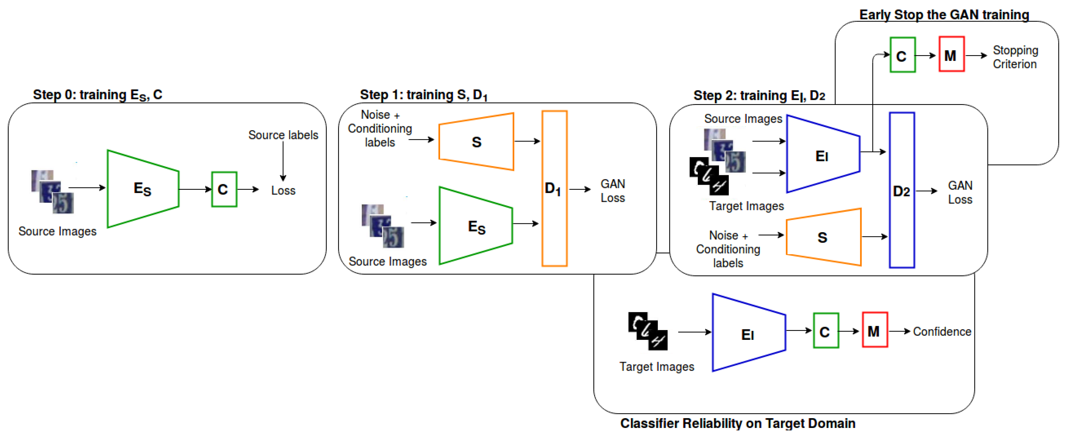
4.1. Domain Adaptation Network

The experiments were based on the domain adaptation network proposed in [13], whose architecture is depicted in Figure 1.
Specifically, the network employs a classifier C, which is attached on the top of a feature extractor E S , and trained on the source dataset (Step 0). After that, S, the generator of a conditional GAN (CGAN [45]), is used to learn the distribution of the features extracted by E S from the source dataset (Step 1). Finally, a second GAN is used to train another feature encoder, E I , aimed at extracting the same feature distribution from both the source and the target domain (Step 2). In this step, E I acts as the GAN generator and learns to match the feature distribution produced by S (its weights are not updated in this phase). The procedure aims at extracting features from the target domain that are indistinguishable from those extracted from the source domain. Therefore, based on the features extracted by E I , the classifier C can be used to classify images in the target domain. The training procedure proposed by Volpi et al. [13] was modified as follows:
  • Step 0. The validation set of the source domain is used to early stop the training.
  • Step 1. The CGAN generator, S, produces features for a given class; then, every 1000 training steps, C is engaged in classifying the features generated by S, using the conditioning labels to evaluate the error and early stop the training.
  • Step 2. Every 1000 iteration, the classifier C is used to classify the features extracted from E I . The proposed confidence measures are used to evaluate the performance of the classifier to early stop the training.
In the task of SVHN → MNIST, the network hyper-parameters (number of layers, initial weights, learning rate, batch size, etc.) are the same as in [13], while for CIFAR → STL, which is not utilized in [13], the same network structure is maintained, changing only the weight initialization (truncated norm), the pooling kernel size (from 2 to 3), and using the padding “same” instead of “valid” in the feature extractor convolutions. (The type “same” means using zero-padding in order to have an output feature map with the same size of the input. Instead, “valid” means no padding is added and the convolution is applied only inside the feature map; in this case, the resulting feature map size is reduced depending on the size of the convolutional kernel.)

4.2. Datasets

To evaluate the proposed confidence measures, we used two public source/target benchmark datasets, typically adopted in domain adaptation.

4.2.1. SVHN → MNIST

Street View House Numbers (SVHN) [15] is a dataset containing real images of house numbers taken from Google Street View. Instead, MNIST [16] collects images of handwritten digits. MNIST images were resized to 32 × 32 pixels and SVHN images were converted to gray-scale. A subset of images taken from the extra set of SVHN was used as the validation set, to early stop the training of the Step 0 and to compute the thresholds for the confidence measures.

4.2.2. CIFAR → STL

Both CIFAR-10 [17] and STL-10 [18] are 10-class image datasets with nine overlapping classes. Following the procedure described in [57], we removed the non-overlapping classes “frog” and “monkey”, and reduced the problem to a nine-class classification problem. STL images were resized to 32 × 32 and a subset of the training set of CIFAR-10 was used as the validation set, to early stop the training of Step 0 and to compute the thresholds for the confidence measures.

4.3. Network Training

Each experiment was carried out following the same setup, based on the network architecture reported in Figure 1. Firstly, E S and C were trained on the source dataset, then E S was used in Step 1 to train the feature generator S. The validation set of the source domain was used to compute the scale factor T needed for both the confidence measures e and s (see Equations (3) and (4)). Features extracted by E S from the validation set were then used to train an auto-encoder for each class, to compute d f e a t and C B P (see Equations (8) and (9)). Each measure was used to evaluate the reliability of the classifier, predicting whether the network C would correctly classify the sample or not. For this purpose, a threshold for each measure needed to be set to discriminate certain and uncertain samples. Threshold values were selected to maximize the accuracy on the validation set of the source domain, based on the Receiver Operating Characteristic (ROC) (the ROC is a graphical plot that displays, at different thresholds, the true positive rate against the false positive rate achieved by a binary classifier) obtained using a balanced subset of 5000 classified/misclassified samples (see Figure 2 and Figure 3).
The obtained thresholds were also used at the end of the adaptation procedure to evaluate the reliability of the classifier on the target domain. Finally, E I was trained on the target domain using the GAN of Step 2. In this phase, every 1000 iterations, features extracted from the target domain by E I were fed into the classifier C. The reliability estimator M, a regressors that computes one of the proposed confidence measures, was used to decide when stopping the training.

5. Results

Section 5.1 reports the experimental results obtained using the proposed confidence measures to stop the training of the GAN in Step 2, whereas Section 5.2 illustrates the results achieved when the confidence measures were employed to evaluate the reliability of the classifier after the domain adaptation phase.

5.1. Early Stop of the GAN Training

In domain adaptation process, the labels of the target domain are not available. For this reason, a validation set cannot be used to evaluate the training progress; normally, a fixed number of training step is set to stop the domain adaptation phase. This criterion does not guarantee stopping the training properly, especially if the training is not stable. The proposed confidence measures proved to be related to the performance of a classifier and, in addition, they did not require the labels of the target dataset to be computed. For these reasons, our idea was to use them to monitor the domain adaptation process and to stop the training properly. In particular, the proposed confidence measures could be used to stop the training of the GAN in Step 2. In this GAN, the generator E I was initialized with the pre-trained weights of E S and was fed with a combination of images from both the target and the source domain. E I was trained to learn the feature distribution produced by S (the generator of the GAN in Step 1). This particular configuration seemed to guarantee much more stability than a classic GAN framework. To prove the effectiveness of the proposed measures in GAN the training, the following experimental setup was employed:
  • The training was stopped according to the confidence measures (e, s, d i m g , g, d f e a t , m i x 1 and m i x 2 ) computed by the reliability estimator M.
  • The GAN was trained for a fixed number (200,000) of iterations (Fix Iter.).
  • The early stop was based on the accuracy calculated on the validation set (Max Acc.)
The experiments aimed at comparing the performance of the classifier C, when the GAN was stopped according to these different strategies. It is worth noting that the stopping criterion based on the use of a validation set was not feasible in domain adaptation and, in this work, it was used only for comparison purposes, since it provided an ideal optimal performance. The experiments were carried out on two domain adaptation tasks: SVHN → MNIST and CIFAR10 → STL.

5.1.1. SVHN → MNIST

In this experimental setup, SVHN was used as the source domain and MNIST as the target domain. The experiments were repeated 20 times to obtain statistically reliable results. Table 1 reports the accuracy obtained using different measures as stopping criteria. Instead, Table 2 shows the mean and the standard deviation of the difference between the accuracy obtained with the use of a validation set (theoretical optimum) and the proposed measures.

5.1.2. CIFAR → STL

In this experimental setup, CIFAR was used as the source domain and STL as the target domain. As in SVHN → MNIST, the experiments were repeated 20 times to obtain more statistically reliable results. Table 3 shows the accuracy obtained using different measures as stopping criteria. Instead, Table 4 displays the mean and the standard deviation of the difference between the accuracy obtained with the use of a validation set (theoretical optimum) and the proposed measures.
The experiments showed that the proposed confidence measures allow stopping the domain adaptation process when the accuracy was close to the performance that could be obtained only with a labeled validation set. Moreover, the obtained accuracy was better than the one achievable using a fixed number of iterations. It is also worth mentioning that, in our experiments, the training of the GAN tended to converge, while, in those cases when this favorable condition was not satisfied, the proposed measures might become even more effective. Furthermore, in both experimental setups, the best results were obtained using a combined measure. This suggests that different measures captured different information about the network output uncertainty. Here, measures were combined simply computing their mean (see Section 3.4), whereas it is a matter of future work to evaluate more complicated combination strategies.

5.2. Classifier Reliability

In a real domain adaptation setting, the performance of the classifier C cannot be evaluated, since a labeled test set is not available. Instead, the proposed confidence measures allow estimating the reliability of classifier C on target samples. Formally, a reliability classifier M, implementing one of the proposed measures, estimated the confidence of the output of C. For each confidence measure, a threshold t h was employed, on the output of M, to classify the network output as certain or uncertain. If the confidence provided by M was larger than t h , then the output of C was considered to be reliable; otherwise, it was considered unreliable. In the experiments, t h was set based on the ROC, using each measure to predict the accuracy on the validation set of the source dataset (see Figure 2 and Figure 3). Table 5 and Table 6 show the accuracy and the Area Under the ROC (AUROC) achieved by M on the test set of the target domain. (The area under the ROC is a measure of the performance of the classifier. Differently from the accuracy, the AUROC does not depend on a single predefined threshold, but it provides a unique measure that summarizes the behavior of the classifier for each possible thresholds.) In Table 7 and Table 8, the corresponding confusion matrices are shown. On SVHN → MNIST, the best reliability classifier M obtained an accuracy of about 89% and an AUROC of about 73%. Notice that, in this case, the accuracy was not a significant metric because the classifier C was very accurate and therefore correctly and incorrectly classified samples are unbalanced (i.e., we would obtain an accuracy of 92.34% only classifying each instance as “certain”). However, the value of the AUROC suggests that the proposed confidence values are correlated to the errors of C. The benchmark CIFAR → STL was more challenging and, in fact, the network proposed by Volpi et al. [13] reached an accuracy of just 56% on STL. In this case, our measures allowed predicting the correctness of the output with an accuracy of about 67% and an AUROC of about 73%. Thus, the experiments suggested that the proposed confidence measures are closely related with the actual reliability of the classifier, and could be very useful where an accurate uncertainty estimation is fundamental for decision making, such as in automatic analysis of medical images.

6. Conclusions

We investigated the use of confidence measures in domain adaptation to stop the training of a GAN and to evaluate the reliability of the classifier on the target domain. The results show that the proposed measures allowed early stopping the training, nonetheless approaching the optimum, which could only be reached when a labeled validation set is available. Moreover, confidence measures can also be used to accurately estimate the reliability of the image classifier. Finally, simply mixing (based on an average operation) different confidence measures allowed capturing different types of network uncertainty, refining the reliability estimation, whereas it is a matter of future work to consider more targeted combination strategies. It will be also interesting to assess the proposed approach within different domain adaptation frameworks and with different benchmarks, particularly in decision support systems for medical imaging, where the uncertainty assessment of a predictive model is mandatory.

Author Contributions

Conceptualization, S.B. and A.P.; Formal analysis, S.B. and P.A.; Investigation, S.B., P.A., M.B. and F.S.; Methodology, S.B. and P.A.; Software, S.B.; Supervision, M.B., A.P. and F.S.; Validation, S.B.; Writing—original draft, S.B. and P.A.; and Writing—review and editing, S.B., P.A., M.B., A.P. and F.S.

Funding

This research received no external funding.

Acknowledgments

Work done during internship at the University of Copenhagen. Authors wish to acknowledge the CINECA award, under the ISCRA initiative, for the availability of high-performance computing resources and support.

Conflicts of Interest

The authors declare no conflict of interest.

References

  1. Girshick, R.; Donahue, J.; Darrell, T.; Malik, J. Rich feature hierarchies for accurate object detection and semantic segmentation. In Proceedings of the IEEE Conference on Computer Vision and Pattern Recognition, Columbus, OH, USA, 23–28 June 2014; pp. 580–587. [Google Scholar]
  2. Long, J.; Shelhamer, E.; Darrell, T. Fully convolutional networks for semantic segmentation. In Proceedings of the IEEE Conference on Computer Vision and Pattern Recognition, Boston, MA, USA, 7–12 June 2015; pp. 3431–3440. [Google Scholar]
  3. Chen, L.C.; Papandreou, G.; Kokkinos, I.; Murphy, K.; Yuille, A.L. Semantic image segmentation with deep convolutional nets and fully connected CRFs. arXiv 2014, arXiv:1412.7062. [Google Scholar]
  4. Amodei, D.; Ananthanarayanan, S.; Anubhai, R.; Bai, J.; Battenberg, E.; Case, C.; Casper, J.; Catanzaro, B.; Cheng, Q.; Chen, G.; et al. Deep speech 2: End–to–end speech recognition in English and Mandarin. In Proceedings of the International Conference on Machine Learning, New York, NY, USA, 19–24 June 2016; pp. 173–182. [Google Scholar]
  5. Caruana, R.; Lou, Y.; Gehrke, J.; Koch, P.; Sturm, M.; Elhadad, N. Intelligible models for healthcare: Predicting pneumonia risk and hospital 30-day readmission. In Proceedings of the 21th ACM SIGKDD International Conference on Knowledge Discovery and Data Mining, Sydney, NSW, Australia, 10–13 August 2015; pp. 1721–1730. [Google Scholar]
  6. Andreini, P.; Bonechi, S.; Bianchini, M.; Mecocci, A.; Scarselli, F. A Deep Learning Approach to Bacterial Colony Segmentation. In Proceedings of the International Conference on Artificial Neural Networks, Rhodes, Greece, 4–7 October 2018; pp. 522–533. [Google Scholar]
  7. Deng, J.; Dong, W.; Socher, R.; Li, L.J.; Li, K.; Fei-Fei, L. Imagenet: A large–scale hierarchical image database. In Proceedings of the IEEE Conference on Computer Vision and Pattern Recognition, Miami, FL, USA, 20–25 June 2009; pp. 248–255. [Google Scholar]
  8. Gretton, A.; Smola, A.J.; Huang, J.; Schmittfull, M.; Borgwardt, K.M.; Schölkopf, B. Covariate Shift by Kernel Mean Matching; MIT Press: Cambridge, MA, USA, 2009. [Google Scholar]
  9. Donahue, J.; Jia, Y.; Vinyals, O.; Hoffman, J.; Zhang, N.; Tzeng, E.; Darrell, T. Decaf: A deep convolutional activation feature for generic visual recognition. In Proceedings of the International Conference on Machine Learning, Beijing, China, 21–26 June 2014; pp. 647–655. [Google Scholar]
  10. Torralba, A.; Efros, A.A. Unbiased look at dataset bias. In Proceedings of the 2011 IEEE Conference on Computer Vision and Pattern Recognition (CVPR), Colorado Springs, CO, USA, 20–25 June 2011; pp. 1521–1528. [Google Scholar]
  11. Ben-David, S.; Blitzer, J.; Crammer, K.; Pereira, F. Analysis of representations for domain adaptation. In Advances in Neural Information Processing Systems; MIT Press: Cambridge, MA, USA, 2007; pp. 137–144. [Google Scholar]
  12. Goodfellow, I.; Pouget-Abadie, J.; Mirza, M.; Xu, B.; Warde-Farley, D.; Ozair, S.; Courville, A.; Bengio, Y. Generative adversarial nets. In Advances in Neural Information Processing Systems; MIT Press: Cambridge, MA, USA, 2014; pp. 2672–2680. [Google Scholar]
  13. Volpi, R.; Morerio, P.; Savarese, S.; Murino, V. Adversarial feature augmentation for unsupervised domain adaptation. In Proceedings of the IEEE Conference on Computer Vision and Pattern Recognition (CVPR), Salt Lake City, UT, USA, 18–22 June 2018. [Google Scholar]
  14. Smith, L.; Gal, Y. Understanding Measures of Uncertainty for Adversarial Example Detection. arXiv 2018, arXiv:1803.08533. [Google Scholar]
  15. Netzer, Y.; Wang, T.; Coates, A.; Bissacco, A.; Wu, B.; Ng, A.Y. Reading digits in natural images with unsupervised feature learning. In NIPS Workshop on Deep Learning and Unsupervised Feature Learning; NIPS: San Diego, CA, USA, 2011; Volume 2011, p. 5. [Google Scholar]
  16. LeCun, Y.; Bottou, L.; Bengio, Y.; Haffner, P. Gradient-based learning applied to document recognition. Proc. IEEE 1998, 86, 2278–2324. [Google Scholar] [CrossRef] [Green Version]
  17. Krizhevsky, A.; Hinton, G. Learning Multiple Layers of Features from Tiny Images; Technical report; University of Toronto: Toronto, ON, Canada, 2009. [Google Scholar]
  18. Coates, A.; Ng, A.; Lee, H. An analysis of single–layer networks in unsupervised feature learning. In Proceedings of the Fourteenth International Conference on Artificial Intelligence and Statistics, Fort Lauderdale, FL, USA, 11–13 April 2011; pp. 215–223. [Google Scholar]
  19. Saenko, K.; Kulis, B.; Fritz, M.; Darrell, T. Adapting visual category models to new domains. In Proceedings of the European Conference on Computer Vision, Crete, Greece, 5–11 September 2010; pp. 213–226. [Google Scholar]
  20. Jhuo, I.H.; Liu, D.; Lee, D.; Chang, S.F. Robust visual domain adaptation with low–rank reconstruction. In Proceedings of the 2012 IEEE Conference on Computer Vision and Pattern Recognition (CVPR), Providence, RI, USA, 16–21 June 2012; pp. 2168–2175. [Google Scholar]
  21. Hoffman, J.; Rodner, E.; Donahue, J.; Darrell, T.; Saenko, K. Efficient learning of domain–invariant image representations. arXiv 2013, arXiv:1301.3224. [Google Scholar]
  22. Sun, B.; Saenko, K. Deep coral: Correlation alignment for deep domain adaptation. In Proceedings of the European Conference on Computer Vision, Amsterdam, The Netherlands, 8–16 October 2016; pp. 443–450. [Google Scholar]
  23. Long, M.; Cao, Y.; Wang, J.; Jordan, M.I. Learning transferable features with deep adaptation networks. arXiv 2015, arXiv:1502.02791. [Google Scholar]
  24. Long, M.; Zhu, H.; Wang, J.; Jordan, M.I. Unsupervised domain adaptation with residual transfer networks. In Advances in Neural Information Processing Systems; NIPS: San Diego, CA, USA, 2016; pp. 136–144. [Google Scholar]
  25. Haeusser, P.; Frerix, T.; Mordvintsev, A.; Cremers, D. Associative domain adaptation. In Proceedings of the International Conference on Computer Vision (ICCV), Italy, France, 22–27 October 2017; Volume 2, p. 6. [Google Scholar]
  26. Luo, Z.; Zou, Y.; Hoffman, J.; Fei-Fei, L.F. Label efficient learning of transferable representations acrosss domains and tasks. In Advances in Neural Information Processing Systems; NIPS: San Diego, CA, USA, 2017; pp. 165–177. [Google Scholar]
  27. Ganin, Y.; Ustinova, E.; Ajakan, H.; Germain, P.; Larochelle, H.; Laviolette, F.; Marchand, M.; Lempitsky, V. Domain-adversarial training of neural networks. J. Mach. Learn. Res. 2016, 17, 1–35. [Google Scholar]
  28. Tzeng, E.; Hoffman, J.; Darrell, T.; Saenko, K. Simultaneous deep transfer across domains and tasks. In Proceedings of the IEEE International Conference on Computer Vision, Santiago, Chile, 7–13 December 2015; pp. 4068–4076. [Google Scholar]
  29. Ganin, Y.; Lempitsky, V. Unsupervised domain adaptation by backpropagation. In Proceedings of the 32nd International Conference on Machine Learning, Lille, France, 6–11 July 2015; pp. 1180–1189. [Google Scholar]
  30. Tzeng, E.; Hoffman, J.; Saenko, K.; Darrell, T. Adversarial discriminative domain adaptation. In Proceedings of the IEEE Conference on Computer Vision and Pattern Recognition (CVPR), Honolulu, HI, USA, 21–26 July 2017; Volume 1, p. 4. [Google Scholar]
  31. Damodaran, B.B.; Kellenberger, B.; Flamary, R.; Tuia, D.; Courty, N. DeepJDOT: Deep Joint distribution optimal transport for unsupervised domain adaptation. In Proceedings of the European Conference on Computer Vision (ECCV), Munich, Germany, 8–14 September 2018; Volume 11208. [Google Scholar]
  32. Shu, R.; Bui, H.; Narui, H.; Ermon, S. A DIRT–T Approach to Unsupervised Domain Adaptation. In Proceedings of the International Conference on Learning Representations, Vancouver, BC, Canada, 30 April–3 May 2018. [Google Scholar]
  33. Taigman, Y.; Polyak, A.; Wolf, L. Unsupervised cross-domain image generation. In Proceedings of the International Conference on Learning Representations (ICLR), Toulon, France, 24–26 April 2017. [Google Scholar]
  34. Liu, M.Y.; Tuzel, O. Coupled generative adversarial networks. In Advances in Neural Information Processing Systems; NIPS: San Diego, CA, USA, 2016; pp. 469–477. [Google Scholar]
  35. Bousmalis, K.; Silberman, N.; Dohan, D.; Erhan, D.; Krishnan, D. Unsupervised pixel–level domain adaptation with generative adversarial networks. In Proceedings of the IEEE Conference on Computer Vision and Pattern Recognition (CVPR), Honolulu, HI, USA, 21–26 July 2017; Volume 1, p. 7. [Google Scholar]
  36. Liu, M.Y.; Breuel, T.; Kautz, J. Unsupervised image–to–image translation networks. In Advances in Neural Information Processing Systems; NIPS: San Diego, CA, USA, 2017; pp. 700–708. [Google Scholar]
  37. Sankaranarayanan, S.; Balaji, Y.; Castillo, C.D.; Chellappa, R. Generate to adapt: Aligning domains using generative adversarial networks. arXiv 2017, arXiv:1704.01705. [Google Scholar]
  38. Murez, Z.; Kolouri, S.; Kriegman, D.J.; Ramamoorthi, R.; Kim, K. Image to Image Translation for Domain Adaptation. In Proceedings of the IEEE Conference on Computer Vision and Pattern Recognition (CVPR), Honolulu, HI, USA, 21–26 July 2017. [Google Scholar]
  39. Mao, X.; Li, Q.; Xie, H.; Lau, R.Y.; Wang, Z.; Smolley, S.P. Least squares generative adversarial networks. In Proceedings of the 2017 IEEE International Conference on Computer Vision (ICCV), Venice, Italy, 22–29 October 2017; pp. 2813–2821. [Google Scholar]
  40. Arjovsky, M.; Chintala, S.; Bottou, L. Wasserstein generative adversarial networks. In Proceedings of the International Conference on Machine Learning, Sydney, Australia, 11–15 August 2017; pp. 214–223. [Google Scholar]
  41. Karras, T.; Aila, T.; Laine, S.; Lehtinen, J. Progressive Growing of GANs for Improved Quality, Stability, and Variation. In Proceedings of the International Conference on Learning Representations, Vancouver, BC, Canada, 30 April–3 May 2018. [Google Scholar]
  42. Salimans, T.; Goodfellow, I.; Zaremba, W.; Cheung, V.; Radford, A.; Chen, X. Improved techniques for training GANs. In Advances in Neural Information Processing Systems; NIPS: San Diego, CA, USA, 2016; pp. 2234–2242. [Google Scholar]
  43. Chen, X.; Duan, Y.; Houthooft, R.; Schulman, J.; Sutskever, I.; Abbeel, P. Infogan: Interpretable representation learning by information maximizing generative adversarial nets. In Advances in Neural Information Processing Systems; NIPS: San Diego, CA, USA, 2016; pp. 2172–2180. [Google Scholar]
  44. Reed, S.E.; Akata, Z.; Mohan, S.; Tenka, S.; Schiele, B.; Lee, H. Learning what and where to draw. In Advances in Neural Information Processing Systems; NIPS: San Diego, CA, USA, 2016; pp. 217–225. [Google Scholar]
  45. Mirza, M.; Osindero, S. Conditional generative adversarial nets. arXiv 2014, arXiv:1411.1784. [Google Scholar]
  46. Neal, R.M. Bayesian Learning for Neural Networks; Springer Science & Business Media: Berlin, Germany, 2012; Volume 118. [Google Scholar]
  47. Gal, Y.; Ghahramani, Z. Dropout as a Bayesian approximation: Representing model uncertainty in deep learning. In Proceedings of the International Conference on Machine Learning, New York City, NY, USA, 19–24 June 2016; pp. 1050–1059. [Google Scholar]
  48. Louizos, C.; Welling, M. Multiplicative Normalizing Flows for Variational Bayesian Neural Networks. In Proceedings of the International Conference on Machine Learning, Sydney, Australia, 11–15 August 2017. [Google Scholar]
  49. Atanov, A.; Ashukha, A.; Molchanov, D.; Neklyudov, K.; Vetrov, D. Uncertainty Estimation via Stochastic Batch Normalization. In Proceedings of the International Conference on Learning Representations, Vancouver, BC, Canada, 30 April–3 May 2018. [Google Scholar]
  50. Lakshminarayanan, B.; Pritzel, A.; Blundell, C. Simple and scalable predictive uncertainty estimation using deep ensembles. In Advances in Neural Information Processing Systems; NIPS: San Diego, CA, USA, 2017; pp. 6402–6413. [Google Scholar]
  51. Kendall, A.; Gal, Y. What uncertainties do we need in bayesian deep learning for computer vision? In Advances in Neural Information Processing Systems; NIPS: San Diego, CA, USA, 2017; pp. 5574–5584. [Google Scholar]
  52. DeVries, T.; Taylor, G.W. Learning Confidence for Out–of–Distribution Detection in Neural Networks. arXiv 2018, arXiv:1802.04865. [Google Scholar]
  53. DeVries, T.; Taylor, G.W. Leveraging Uncertainty Estimates for Predicting Segmentation Quality. arXiv 2018, arXiv:1807.00502. [Google Scholar]
  54. Guo, C.; Pleiss, G.; Sun, Y.; Weinberger, K.Q. On calibration of modern neural networks. arXiv 2017, arXiv:1706.04599. [Google Scholar]
  55. Mallidi, S.H.; Ogawa, T.; Hermansky, H. Uncertainty estimation of DNN classifiers. In Proceedings of the 2015 IEEE Workshop on Automatic Speech Recognition and Understanding (ASRU), Scottsdale, AZ, USA, 13–17 December 2015; pp. 283–288. [Google Scholar]
  56. Goodfellow, I.J.; Shlens, J.; Szegedy, C. Explaining and Harnessing Adversarial Examples. arXiv 2014, arXiv:1412.6572. [Google Scholar]
  57. French, G.; Mackiewicz, M.; Fisher, M. Self–ensembling for visual domain adaptation. arXiv 2017, arXiv:1706.05208. [Google Scholar]
Figure 1. Domain adaptation network architecture.
Applsci 09 02192 g001
Figure 2. ROC curves obtained using each measures to predict the accuracy on the SVHN validation set. Measures e, s, d i m g , g, d f e a t , m i x 1 and m i x 2 are, respectively, plotted in (ag).
Applsci 09 02192 g002
Figure 3. ROC curves obtained using each measures to predict the accuracy on the CIFAR validation set. Measures e, s, d i m g , g, d f e a t , m i x 1 and m i x 2 are, respectively, plotted in (ag).
Applsci 09 02192 g003
Table 1. Accuracy (Acc.) on the MNIST test set obtained stopping the training with different strategies (the experiments were repeated 20 times and the accuracies were averaged).
Max Acc.Fix Iter.es d img g d feat CBP mix 1 mix 2
Acc.92.34%91.67%91.81%91.79%91.56%91.80%91.65%91.66%91.87%91.79%
Table 2. Mean and standard deviation of the difference between the accuracy obtained with the use of a validation set and the proposed measures on the MNIST test set.
Max Acc.Fix Iter.es d img g d feat CBP mix 1 mix 2
Mean-0.67%0.53%0.56%0.78%0.54%0.69%0.68%0.47%0.55%
Std-0.270.290.260.470.300.340.310.210.25
Table 3. Average accuracy (Acc.) on the STL test set obtained stopping the training with different strategies (the experiments were repeated 20 times and the accuracies were averaged).
Max Acc.Fix Iter.es d img g d feat CBP mix 1 mix 2
Acc.56.81%55.90%56.08%56.04%55.92%55.94%55.95%56.04%56.06%56.18%
Table 4. Mean and standard deviation of the difference between the accuracy obtained with the use of a validation set and the proposed measures on STL test set.
Max Acc.Fix Iter.es d img g d feat CBP mix 1 mix 2
Mean-0.91%0.73%0.77%0.89%0.87%0.86%0.77%0.75%0.63%
Std-0.330.330.360.350.420.360.240.330.33
Table 5. Accuracy and AUROC of the uncertainty prediction on the MNIST test set.
es d img g d feat CBP mix 1 mix 2
Accuracy89.44%89.15%86.99%88.37%82.27%91.36%87.94%83.28%
AUROC71.21%72.90%73.21%66.58%63.22%52.75%69.39%67.79%
Table 6. Accuracy and AUROC of the uncertainty prediction on the STL test set.
es d img g d feat CBP mix 1 mix 2
Accuracy67.22%67.45%65.80%66.56%67.01%58%67.70%66.77%
AUROC68.32%72.82%72.20%73.08%73.10%51.99%73.39%72.60%
Table 7. Confusion matrices on MNIST, where CC and IC are the correctly and incorrectly classified samples, respectively.
es d img g
CCICCCICCCICCCIC
Certain8646517860950983244408515493
Uncertain539298576306861375670322
d feat CBP mix 1 mix 2
CCICCCICCCICCCIC
Certain7918506908277184704918101588
Uncertain1267309103547153241084227
Table 8. Confusion matrices on STL, where CC and IC are the correctly and incorrectly classified samples, respectively.
es d img g
CCICCCICCCICCCIC
Certain2913120928331112230570329811324
Uncertain11511927123120241759243310831812
d feat CBP mix 1 mix 2
CCICCCICCCICCCIC
Certain29721283400629662885114629391267
Uncertain10921853581701179199011251869

