Article

Multiscale Superpixelwise Locality Preserving Projection for Hyperspectral Image Classification

1
School of Automation Science and Engineering, South China University of Technology, Guangzhou 510640, China
2
Guangdong Provincial Key Laboratory of Urbanization and Geo-Simulation, Center of Integrated Geographic Information Analysis, School of Geography and Planning, Sun Yat-sen University, Guangzhou 510275, China
3
Mechanical and Electrical Engineering College, Hainan University, Haikou 570228, China
*
Authors to whom correspondence should be addressed.
Appl. Sci. 2019, 9(10), 2161; https://doi.org/10.3390/app9102161
Submission received: 31 March 2019 / Revised: 21 May 2019 / Accepted: 22 May 2019 / Published: 27 May 2019

Abstract

:
Manifold learning is a powerful dimensionality reduction tool for a hyperspectral image (HSI) classification to relieve the curse of dimensionality and to reveal the intrinsic low-dimensional manifold. However, a specific characteristic of HSIs, i.e., irregular spatial dependency, is not taken into consideration in the method design, which can yield many spatially homogenous subregions in an HSI scence. Conventional manifold learning methods, such as a locality preserving projection (LPP), pursue a unified projection on the entire HSI, while neglecting the local homogeneities on the HSI manifold caused by those spatially homogenous subregions. In this work, we propose a novel multiscale superpixelwise LPP (MSuperLPP) for HSI classification to overcome the challenge. First, we partition an HSI into homogeneous subregions with a multiscale superpixel segmentation. Then, on each scale, subregion specific LPPs and the associated preliminary classifications are performed. Finally, we aggregate the classification results from all scales using a decision fusion strategy to achieve the final result. Experimental results on three real hyperspectral data sets validate the effectiveness of our method.

1. Introduction

Hyperspectral image (HSI) classification has been a research hotspot over recent years, since it plays a critical role in military target detection, precision agriculture, mine exploration, and many other applications [1,2,3]. With abundant spectral information, HSIs show great potential in identifying different ground objects of interest. However, hundreds of spectral bands in an HSI also bring about some problems, such as heavy computation burdens and the Hughes phenomenon which means that a large amount of training HSI pixels are required to maintain statistical confidence in the HSI classification task [4,5]. Such problems usually hinder HSI classifiers from achieving excellent performance in real applications. In fact, HSI spectral bands are strongly correlated; hence, the spectral signature of each HSI pixel can be represented by only a few features [6,7,8]. Therefore, one often-used strategy to overcome the dimensionality dilemma mentioned above is dimensionality reduction which aims to represent the high-dimensional HSI data in a low-dimensional space without losing important information for discriminating tasks.
Numerous dimensionality reduction methods have been developed, which can be roughly categorized into two groups: feature transform and feature selection [9,10]. Feature transform projects the original HSI data into an appropriate low-dimensional space, while feature selection chooses the most representative bands from the HSI. Feature transform gains the advantage over feature selection that it has the potential to maintain the original information in the high-dimensional data during dimensionality reduction and thus generate more discriminative features [11,12]. Principle component analysis (PCA) and linear discriminant analysis (LDA) are two typical feature transform methods. PCA attempts to map the data along the directions of maximal variance [13]. LDA tends to maximize between-class distances and minimize within-class distances in the meantime [14]. Both PCA and LDA just assume that the information contained in high-dimensional data lies on a linear low-dimensional space, whereas nonlinear structures are often exhibited in real HSI data. To cope with the nonlinearities, manifold learning methods were developed. Manifold learning assumes that the high- dimensional data actually lie on a low-dimensional manifold structure, which can be parameterized with a group of identifiable coordinates. One of the most popular manifold methods is locality preserving projection (LPP) which builds a graph to capture geometric structures of data and subsequently establishes a projection from the original data space to the low-dimensional space [15,16,17,18,19]. Other manifold learning approaches include locally linear embedding (LLE) which supposes that the structure represented by the linear combinations of the data’s nearest neighbors is unchanged in both the high-dimensional and the associated low-dimensional spaces [20], isometric mapping (ISOMAP) which utilizes the geodesic distance to perform low-dimensional embedding [21], and local tangent space alignment (LTSA) which aims to recover the intrinsic manifold of data by aligning the local tangent space of each pixel [22].
Irregular spatial dependency is an important characteristic of HSIs, which is caused by the usual occurrences of complex irregular ground objects in HSI scenes. The dependency brings about spatially local homogeneous subregions in different shapes and sizes in an HSI. Such subregions can be detected effectively with appropriate techniques such as superpixel [23,24,25], where pixels in a homogeneous subregion have similar spectral properties but vary relatively significantly across different subregions. Intuitively, such homogeneous subregions would result in local homogeneities on an HSI manifold. However, conventional manifold learning-based HSI dimensionality reduction methods, such as LPP, directly apply a unified projection on the entire HSI, missing those local homogeneities on the HSI manifold. Motivated by such a consideration, we propose a multiscale superpixelwise LPP (MSuperLPP) method for HSI classification in this work. The method is able to deal with spatially local homogeneities in HSIs during dimensionality reduction, thus offering the potential to improving the subsequent classification. To the best of our knowledge, there is no similar work to ours in existing literature, which performs local homogeneity manifold-based HSI dimensionality reduction. Our methods comprise three major phases. First, we segment an HSI into many homogeneous subregions using entropy rate superpixel segmentation (ERS) with a series of scales, which can exploit fully rich spatial dependencies in different shapes and sizes. Next, on each scale, LPP is run on each subregion with spectral-spatial covariance feature, and the obtained low-dimensional features are fed into a preliminary classifier. In the final step, the results on all the scales are aggregated with a decision fusion strategy to yield the final classification result.
The remainder of this paper is organized as follows. In Section 2, we introduce some backgrounds related to the proposed approach. Section 3 gives the details of the proposed MSuperLPP. Section 4 presents the experiment results, and Section 5 provides a summary of this paper.

2. Related Work and Background

Denote an HSI with N pixels and D bands as X = [ x 1 , x 2 , , x N ] R D × N , and the connected data set in a low-dimensional space as Y = [ y 1 , y 2 , , y N ] R d × N , where d D . LPP is a widely used manifold learning method for HSI dimensionality reduction [16,17,18,19,26], while the region covariance descriptor is an effective spectral-spatial feature for HSI classification [26,27,28]. In the following, they are briefly introduced as backgrounds of our proposed method.

2.1. Locality Preserving Projection

LPP builds a graph to obtain the connections among all HSI pixels and then intends to find an optimal projection A to map the original HSI data into a low-dimensional space, while maintaining the local connection relationships [15,16,17,18,19]. Its objective function can be mathematically represented as
min i , j y i y j 2 W i j
and the weight W i j is defined as
W i j = e x i x j 2 2 σ 2 , if x i N ( x j ) or x j N ( x i ) 0 , otherwise
where σ denotes the scale and N ( x i ) stands for the neighbors of x i . Equation (2) measures the similarity or the distance between pixels x i and x i . Under the similarity, the objective in Equation (1) would lead to a heavy penalty if x i and x j are mapped to be far away from each other; thus minimizing it guarantees that a small distance between x i and x j tends to force a small distance between y i and y j . Given a constraint YDY = I , which means removing the arbitrary scaling factor, the aforementioned optimization problem can be further formulated as
arg min A t r ( A T X L X T A ) s . t . A T XD X T A = I
where I is an identity matrix, D is a diagonal matrix with diagonal entries D i i = j W i j , and L = D W is the graph Laplacian matrix. The problem in Equation (3) can be solved by the following generalized eigenvalue formulation:
XL X T a = λ XD X T a
where λ denotes the eigenvalue and eigenvectors corresponding to the d smallest eigenvalues of Equation (4) from the projection matrix A = [ a 1 , a 2 , , a d ] .
In brief, LPP aims to obtain a projection to perform an HSI dimensionality reduction while preserving the neighborhood structure of the data. Besides the standard LPP mentioned above, some considerations such as sparsity, tensor, and orthogonality can be utilized additionally to solve the projection [17,18,19,29].

2.2. Region Covariance Descriptor

Region covariance descriptor has been applied in the computer vision and brain computer interface problem [30,31,32]. Deng et al. introduced the descriptor to HSI processing [26,27,28]. Suppose that X R W × H × D represents the original HSI cube, X i R w × h × D denotes the spatial region around the ith pixel, and s = w × h is size of a spatially local window, then the region covariance descriptor is as follows:
C i = 1 s 1 t = 1 s ( x t μ i ) ( x t μ i ) T
This can be defined as a spectral-spatial feature of X i , where μ i = 1 s t = 1 s x t . Since the covariance feature is connected to a symmetric positive definite matrix and lies on a Riemannian manifold [32], the Log-Euclidean distance metric shown below can measure the similarity between C i and C j :
d L E ( C i , C j ) = log ( C i 1 C j ) F = k = 1 n log 2 λ k 1 / 2
where λ k is the kth eigenvalue of C i 1 C j .
Performing a region covariance descriptor can yield an excellent spectral-spatial covariance feature for HSI classification [26,27,28], which has the advantage of robustness to noise and spectral variabilities over traditional spectral feature (the original spectral signature) [33,34,35].
Following one of the most effective HSI classification routines which comprises three successive phases, i.e., feature extraction, dimensionality reduction, and classification, the combination of various features and various manifold dimensionality reduction ways can yield different HSI manifold learning schemes which can be testified with a subsequent HSI classifier.

3. Proposed Method

A remotely sensed HSI scene usually comprises irregular ground objects in various shapes and sizes, which leads to the irregular spatial dependency characteristic of an HSI, thus leading to the local homogeneities on the connected HSI manifold. In the following, we develop a new method called MSuperLPP to deal with the manifold local homogeneities. Different from a conventional LPP which applies an unified projection on the entire HSI data, our method adaptively determines homogenous subregions and thus the HSI manifold local homogeneity and then employs a divide-and-conquer strategy to perform LPP processing based on those subregions. Therefore, our method is able to fully explore local homogeneities on the HSI manifold and thus collects more useful discriminative information, which poses the potential to enhance the final classification performance.

3.1. Determination of Manifold Local Homogeneity with Multiscale Superpixel Segmentation

Taking into consideration the irregular spatial dependency characteristic of HSIs, we adopt a multiscale superpixel segmentation strategy here to determine the irregular homogeneous subregions in various shapes and sizes in an HSI. ERS can achieve a natural representation of visual scenes [36,37]. It is based on an undirected graph G ( V , E ) where V is the vertex set and E is the edge set. The vertices can be the pixels of an HSI, and then, the weight of an edge measures the similarity of the connected two pixels. Thus, the image segmentation task becomes the problem of how to partition the graph properly. ERS aims to choose a subset S of E which is in the partition of K subgraphs using the following criterion:
max H ( S ) + λ B ( S )
where the entropy rate term H(S) prefers homogeneous clusters, the regularization term B(S) forces the clusters to be of similar sizes, and the weight λ needs to be nonnegative. To solve the optimization problem in Equation (7), Liu et al. gave an efficient greedy algorithm [36]. In our method, we first use PCA to obtain the first principal component of HSI and then perform ERS on the extracted principal component for convenience.
ERS tends to divide the image into subregions of similar sizes once the number of superpixels is given. However, the homogenous subregions in the HSI are in different sizes. That is to say, ERS with a single scale cannot represent the homogeneities well. Therefore, we perform the segmentation in a multiscale way to tackle this issue, where ERS is run with several scales. Specifically, if an HSI is segmented with 2 P + 1 scales, then the number of superpixels on a scale is determined by
N s = ( 2 ) p N s f , p = 0 , ± 1 , ± 2 , , ± P
where p is the index of scales and N s f is the fundamental number of superpixels and given empirically. With a series of scales, the segmentation is expected to adapt homogeneities in various sizes in the scene and to offer the potential to further reduce the impact of an irregular spatial dependency.
A superpixel obtained in the HSI represents spatially homogenous subregions, while different superpixels means there are spectral signature differences to some degree. Such homogenous subregions in an HSI imply that there are local homogeneities on the associated HSI manifold. Thus, we can determine local homogeneities on the connected HSI manifold by performing the multiscale superpixel segmentation.

3.2. Divide-and-Conquer-Based LPP Classification

As local homogeneities on an HSI manifold can be reflected with superpixels, performing an LPP in each superpixel with a superpixel specific projection is expected to preserve the spatially local geometric structure of the data well.
Our method utilizes the region covariance descriptor to construct the graph for an LPP. The descriptor can yield spectral-spatial covariance features more robust to noise and spectral variabilities than the spectral feature [26,27,28]. More specifically, we characterize pixels with their region covariance descriptors, calculate the pairwise distances among pixels in a superpixel with Log-Euclidean distance metric, find the nearest neighbors of the pixels in a superpixel, and compute their similarities as
W i j = e d L E ( C i , C j ) 2 2 σ 2 , if C i N ( C j ) or C j N ( C i ) 0 , otherwise
where N ( C i ) denotes the neighbors of C i . Then, we run an LPP on each superpixel.
After performing the dimensionality reduction on the HSI with 2 P + 1 different segmentation scales, we classify the obtained low-dimensional data on each scale, and then majority voting decision fusion is utilized to aggregate the results from all the scales. Suppose that the classification result on the jth scale for a pixel is l j . Then, the score for the ith class is
N ( i ) = j = 1 2 P + 1 I ( l j = i )
where I ( l j = i ) = 1 , if l j = i 0 , otherwise denotes an indicator function. The final classification result is achieved by
l = arg max i { 1 , 2 , , L } N ( i )
where L is the number of all possible classes. The flowchart of our proposed MSuperLPP for HSI classification is shown in Figure 1, and the connected performing steps can be found in Algorithm 1.    
Algorithm 1 MSuperLPP
Input: HSI X R W × H × D ; scale set N s p = { N i | i = 1 , 2 , , S } obtained by (8); window size s = w × h .
 Extract spectral-spatial covariance features using (5) and perform PCA to extract the first principle component I f .
for i = 1 to S do
   Segment X into N i homogeneous subregions using ERS with I f ;
   for j = 1 to N i do
    Perform LPP in each subregion R ^ j , where the spectral-spatial covariance features are used to search for the k nearest neighbors.
   end for
   Combine the low-dimensional features of all the subregions on the same scale to form the low-dimensional data on this scale. Perform classification on the scales i to get preliminary output T i .
end for
 Aggregate the classification results T i ( i = 1 , 2 , , S ) using (10) and (11).
Output: Final classification result T.

4. Experimental Results

In our experiments, three real HSI data sets are used to evaluate the proposed MSuperLPP. The first one is the Indian Pines data set, which was acquired by the Airborne Visible/Infrared Imaging Spectrometer (AVIRIS) over northwestern Indiana, including 220 spectral bands as well as 145 × 145 pixels, and its available ground-truth data contains 10249 pixels with 16 classes. 40 noisy bands are removed, and the remaining 180 bands are used for experiments. The second one is the Zaoyuan data set, which was collected by the Operational Modular Imaging Spectrometer (OMIS) over the Zaoyuan region, China, in 2001. The data set comprises 137 × 202 pixels and 128 bands covering the region. After removing the noisy bands, 80 bands remain. Moreover, 23821 pixels with 8 classes are used for classification. The last one is the Salinas data set, which was collected by AVIRIS over Salinas Valley, California. The scene used for the experiments comprises 250 × 110 pixels and 224 bands and has 14 testing classes. After removing the noisy bands, 174 bands are Left for the experiments.
For the Indian Pines and Zaoyuan data sets, we randomly choose 5, 10, 30, and 50 pixels per class for training while the other pixels are used for test. Since some classes have a few samples, we select at most half of the total samples. For the Salinas data set, 1, 3, 5, and 10 pixels per class are selected as training samples. After a dimensionality reduction, both the nearest neighbor (NN) classifier and the support vector machine (SVM) with the radial basis function (RBF) kernel are subsequently applied to evaluate the proposed method. The free parameters of the two classifiers are set with cross-validation [38], including the number of nearest neighbors for the NN classifier and the RBF scale and the regularization coefficient for the SVM classifier. We repeat all the classification experiments ten times to avoid random bias, and the average accuracies are presented.
We compare the proposed MSuperLPP with GlobalLPP-SF (global LPP on spectral feature), GlobalLPP-SSCF (global LPP on region convariance descriptor based spectral-spatial covariance feature), SuperLPP-SF (superpixelwise LPP on spectral feature), and SuperLPP-SSCF (superpixelwise LPP on spectral-spatial covariance feature). In our experimental settings, some other parameters are empirically determined as follows. The window’s size of region covariance descriptor is 3 × 3 for GlobalLPP-SSCF, SuperLPP-SSCF, and MSuperLPP. In MSuperLPP, the fundamental number of superpixel N s f is set to 100 for Indian Pines, 40 for Zaoyuan, and 15 for Salinas, while P is set to 4 for all three data sets.
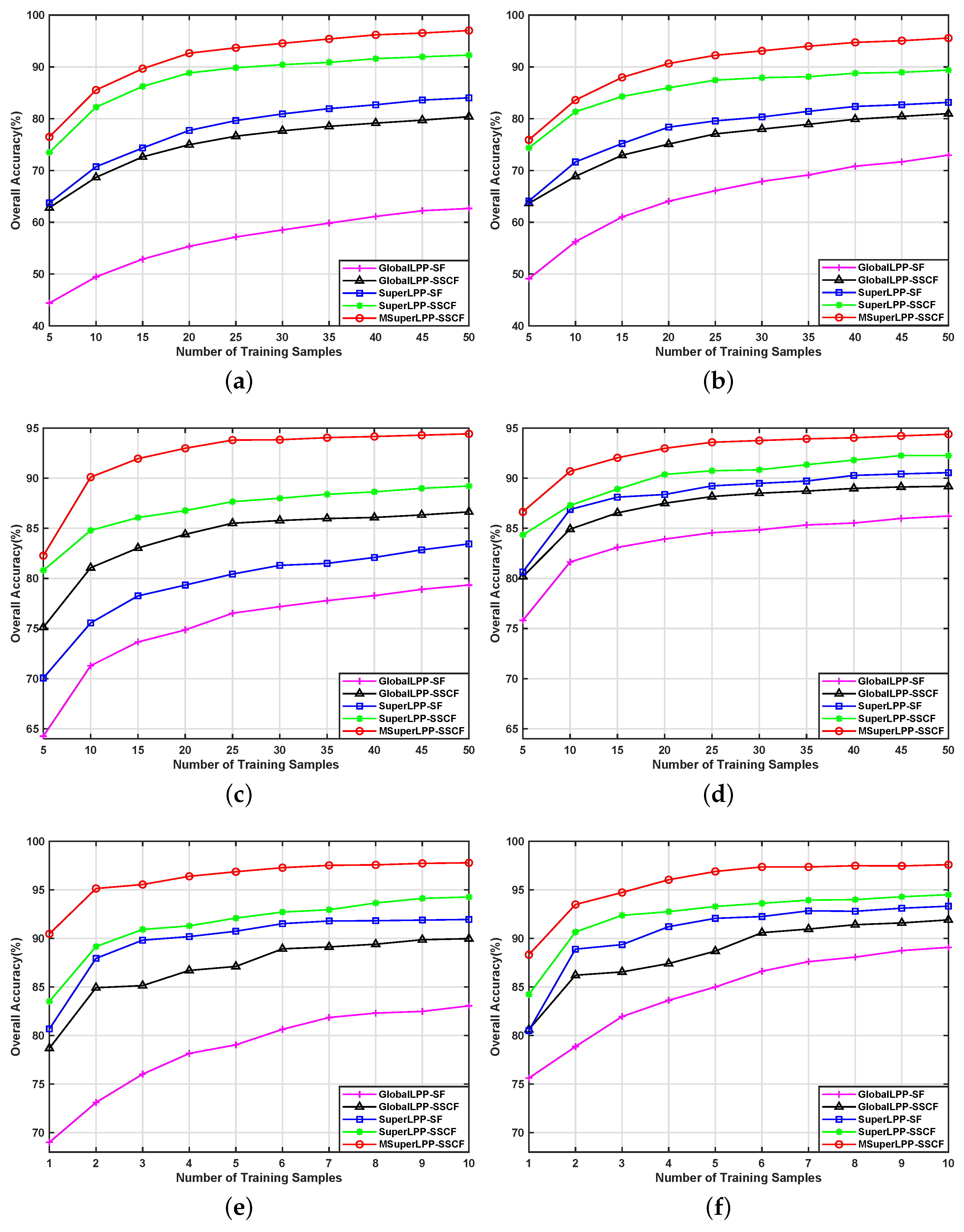
Table 1, Table 2 and Table 3 demonstrate the overall classification accuracies on the Indian Pines, Zaoyuan, and Salinas data sets, respectively. Figure 2 shows the influence of the number of training samples on the classification performance. As observed, GlobalLPP-SSCF performs better than GlobalLPP-SF while SuperLPP-SSCF is better than SuperLPP-SF, which suggests that a spectral-spatial covariance feature is beneficial to improving classification accuracy. Meanwhile, SuperLPP-SSCF and SuperLPP-SF achieve higher accuracies than GlobalLPP-SSCF and GlobalLPP-SF, respectively, which indicates that a superpixel segmentation can enhance classification accuracy. Among all the five considered methods, our proposed MSuperLPP yields the highest accuracies.
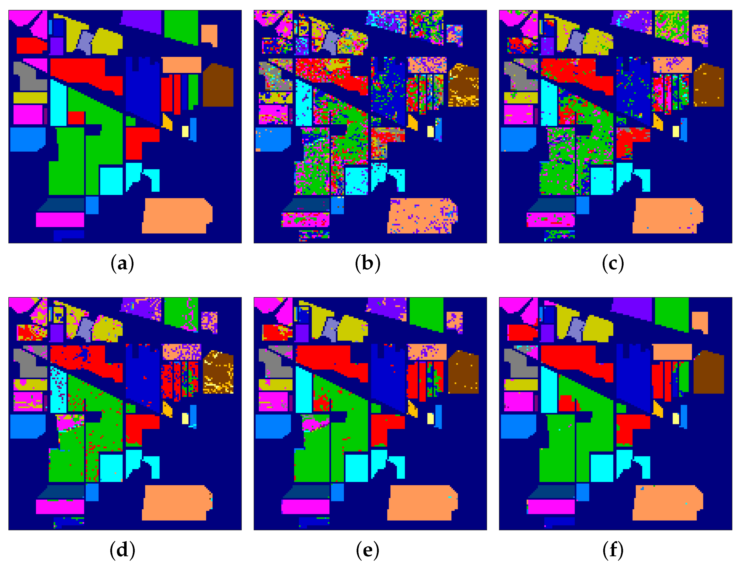
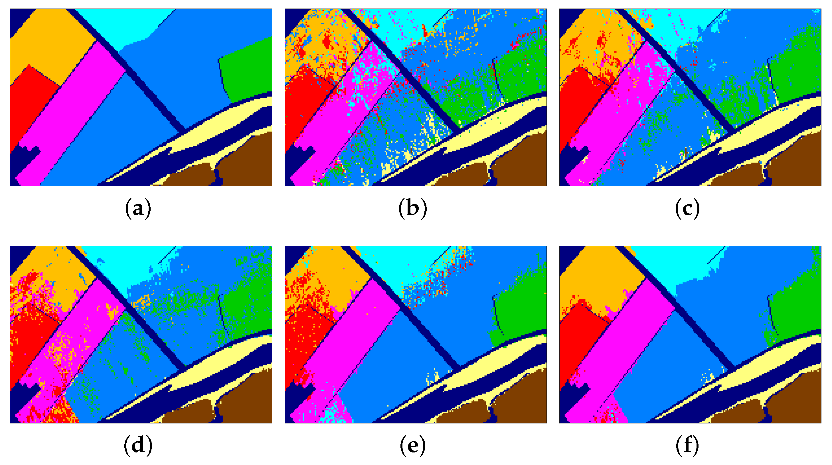
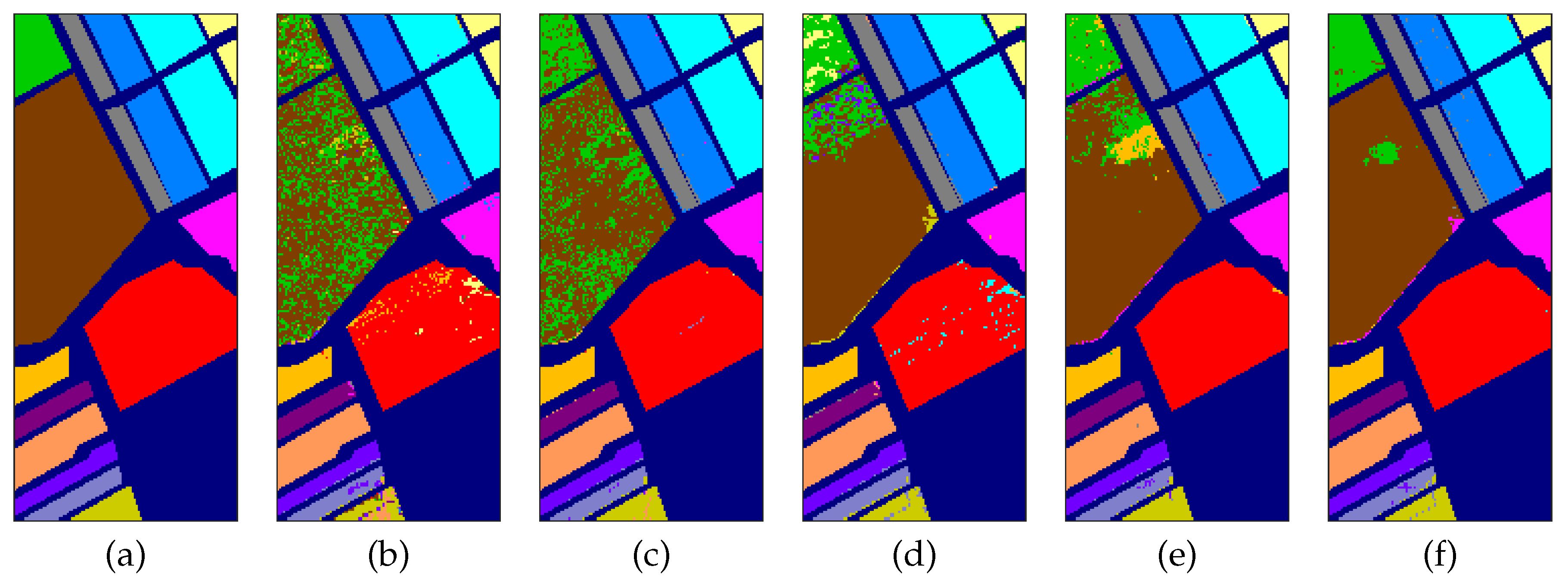
For visual inspection purposes, the classification maps obtained with five compared methods are given in Figure 3, Figure 4 and Figure 5. Here, we only show the results obtained with the nearest neighbor classifier when the size of the training set is set to 50 for Indian Pines and Zaoyuan and 10 for Salinas, respectively. It can be seen that our MSuperLPP yields the best regional consistency and agrees more with the ground truth.
Therefore, it is verified by the experimental results that our MSuperLPP, involving the multiscale superpixel segmentation strategy, is able to achieve an excellent classification performance.

5. Conclusions

Taking into consideration local homogeneities on the HSI manifold connected to the irregular spatial dependency characteristic of an HSI, which is usually ignored by existing manifold learning-based dimensionality reduction methods, we propose a MSuperLPP method for HSI classification. In MSuperLPP, we adopt a divide-and-conquer strategy, first dividing the HSI into many homogeneous subregions on various scales to reveal those local homogeneities, then performing a LPP in each subregion and a preliminary classification on each scale, and finally fusing all the preliminary classification results to yield a final result. The experimental results on real HSI data sets verify the excellent performance of our method.

Author Contributions

All authors made significant contributions to the manuscript. L.H., X.C., and J.L. designed the research framework, conducted the experiments, and wrote the manuscript. L.H. and J.L. were the supervisors of the work and provided the fundings. X.X. provided many constructive suggestions on the motivation analysis and the methodology design.

Funding

This work was supported in part by the National Natural Science Foundation of China under Grant 61571195 and Grant 61771496; in part by the Guangdong Provincial Natural Science Foundation under Grant 2016A030313254, Grant 2016A030313516, and Grant 2017A030313382; and in part by the National Key Research and Development Program of China under Grant 2017YFB0502900.

Conflicts of Interest

The authors declare no conflict of interest.

References

  1. He, L.; Li, J.; Liu, C.Y.; Li, S.T. Recent advances on spectral—Spatial hyperspectral image classification: An overview and new guidelines. IEEE Trans. Geosci. Remote Sens. 2018, 56, 1579–1597. [Google Scholar] [CrossRef]
  2. Chang, C.I. Hyperspectral Data Exploitation: Theory And Applications; John Wiley & Sons: Hoboken, NJ, USA, 2007. [Google Scholar]
  3. Qiu, Z.; Chen, J.; Zhao, Y.; Zhu, S.; He, Y.; Zhang, C. Variety identification of single rice seed using hyperspectral imaging combined with convolutional neural network. Appl. Sci. 2018, 8, 212. [Google Scholar] [CrossRef]
  4. Hughes, G. On the mean accuracy of statistical pattern recognizers. IEEE Transa. Inf. Theory 1968, 14, 55–63. [Google Scholar] [CrossRef]
  5. Thenkabail, P.S.; Gumma, M.K.; Teluguntla, P.; Mohammed, I.A. Hyperspectral remote sensing of vegetation and agricultural crops. Photogramm. Eng. Remote Sens. 2014, 80, 697–723. [Google Scholar]
  6. Jiménez, L.O.; Rivera-Medina, J.L.; Rodríguez-Díaz, E.; Arzuaga-Cruz, E.; Ramírez-Vélez, M. Integration of spatial and spectral information by means of unsupervised extraction and classification for homogenous objects applied to multispectral and hyperspectral data. IEEE Trans. Geosci. Remote Sens. 2005, 43, 844–851. [Google Scholar] [CrossRef]
  7. Ni, D.; Ma, H.B. Classification of hyperspectral image based on sparse representation in tangent space. IEEE Geosci. Remote Sens. Lett. 2015, 12, 786–790. [Google Scholar]
  8. Shao, Z.F.; Zhang, L. Sparse dimensionality reduction of hyperspectral image based on semi-supervised local Fisher discriminant analysis. Int. J. Appl. Earth Obs. Geoinf. 2014, 31, 122–129. [Google Scholar] [CrossRef]
  9. Zhang, L.P.; Zhong, Y.F.; Huang, B.; Gong, J.Y.; Li, P.X. Dimensionality reduction based on clonal selection for hyperspectral imagery. IEEE Trans. Geosci. Remote Sens. 2007, 45, 4172–4186. [Google Scholar] [CrossRef]
  10. Mojaradi, B.; Abrishami-Moghaddam, H.; Zoej, M.J.V.; Duin, R.P. Dimensionality reduction of hyperspectral data via spectral feature extraction. IEEE Trans. Geosci. Remote Sens. 2009, 47, 2091–2105. [Google Scholar] [CrossRef]
  11. Duda, R.O.; Hart, P.E.; Stork, D.G. Pattern Classification; John Wiley & Sons: Hoboken, NJ, USA, 2001. [Google Scholar]
  12. Fukunaga, K. Introduction to Statistical Pattern Recognition; Elsevier: Amsterdam, The Netherlands, 1990. [Google Scholar]
  13. Wold, S.; Esbensen, K.; Geladi, P. Principal component analysis. Chemom. Intell. Lab. Syst. 1987, 2, 37–52. [Google Scholar] [CrossRef]
  14. Bandos, T.V.; Bruzzone, L.; Camps-Valls, G. Classification of hyperspectral images with regularized linear discriminant analysis. IEEE Trans. Geosci. Remote Sens. 2009, 47, 862–873. [Google Scholar] [CrossRef]
  15. He, X.F.; Niyogi, P. Locality preserving projections. In Proceedings of the Annual Conference on Neural Information Processing Systems, Vancouver, BC, Canada, 8–13 December 2003; pp. 153–160. [Google Scholar]
  16. Wang, Z.Y.; He, B.B. Locality perserving projections algorithm for hyperspectral image dimensionality reduction. In Proceedings of the International Conference on Geoinformatics, Shanghai, China, 24–26 June 2011; pp. 1–4. [Google Scholar]
  17. Deng, Y.J.; Li, H.C.; Pan, L.; Emery, W.J. Tensor locality preserving projection for hyperspectral image classification. In Proceedings of the IEEE International Geoscience and Remote Sensing Symposium, Fort Worth, TX, USA, 23–28 July 2017; pp. 771–774. [Google Scholar]
  18. Zhai, Y.; Zhang, L.; Wang, N.; Guo, Y.; Cen, Y.; Wu, T.; Tong, Q. A modified locality-preserving projection approach for hyperspectral image classification. IEEE Geosci. Remote Sens. Lett. 2016, 13, 1059–1063. [Google Scholar] [CrossRef]
  19. Wang, R.; Nie, F.; Hong, R.; Chang, X.; Yang, X.; Yu, W. Fast and orthogonal locality preserving projections for dimensionality reduction. IEEE Trans. Image Process. 2017, 26, 5019–5030. [Google Scholar] [CrossRef]
  20. Roweis, S.T.; Saul, L.K. Nonlinear dimensionality reduction by locally linear embedding. Science 2000, 290, 2323–2326. [Google Scholar] [CrossRef]
  21. Tenenbaum, J.B.; De, S.V.; Langford, J.C. A global geometric framework for nonlinear dimensionality reduction. Science 2000, 290, 2319–2323. [Google Scholar] [CrossRef]
  22. Zhang, Z.Y.; Zha, H.Y. Nonlinear dimension reduction via local tangent space alignment. In Proceedings of the International Conference on Intelligent Data Engineering and Automated Learning, Hong Kong, China, 21–23 March 2003; pp. 477–481. [Google Scholar]
  23. Sun, H.; Ren, J.; Zhao, H.; Yan, Y.; Zabalza, J.; Marshall, S. Superpixel based feature specific sparse representation for spectral-spatial classification of hyperspectral images. Remote Sens. 2019, 11, 536. [Google Scholar] [CrossRef]
  24. Duan, W.; Li, S.; Fang, L. Spectral-spatial hyperspectral image classification using superpixel and extreme learning machines. In Proceedings of the Chinese Conference on Pattern Recognition, Changsha, China, 17–19 November 2014; pp. 159–167. [Google Scholar]
  25. Zhan, T.; Sun, L.; Xu, Y.; Yang, G.; Zhang, Y.; Wu, Z. Hyperspectral classification via superpixel kernel learning-based low rank representation. Remote Sens. 2018, 10, 1639. [Google Scholar] [CrossRef]
  26. Deng, Y.J.; Li, H.C.; Pan, L.; Shao, L.Y.; Du, Q.; Emery, W.J. Modified tensor locality preserving projection for dimensionality reduction of hyperspectral images. IEEE Geosci. Remote Sens. Lett. 2018, 15, 277–281. [Google Scholar] [CrossRef]
  27. Fang, L.; He, N.; Li, S.; Plaza, A.J.; Plaza, J. A new spatial-spectral feature extraction method for hyperspectral images using local covariance matrix representation. IEEE Trans. Geosci. Remote Sens. 2018, 56, 3534–3546. [Google Scholar] [CrossRef]
  28. He, N.; Paoletti, M.E.; Fang, L.; Li, S.; Plaza, A.; Plaza, J. Feature extraction with multiscale covariance maps for hyperspectral image classification. IEEE Trans. Geosci. Remote Sens. 2018, 57, 1–15. [Google Scholar] [CrossRef]
  29. Qiao, L.; Chen, S.; Tan, X. Sparsity preserving projections with applications to face recognition. Pattern Recogn. 2010, 43, 331–341. [Google Scholar] [CrossRef] [Green Version]
  30. Tuzel, O.; Porikli, F.; Meer, P. Pedestrian detection via classification on riemannian manifolds. IEEE Trans. Pattern Anal. Mach. Intell. 2008, 30, 1713–1727. [Google Scholar] [CrossRef]
  31. Xie, X.F.; Yu, Z.L.; Gu, Z.H.; Zhang, J.; Cen, L.; Li, Y.Q. Bilinear regularized locality preserving learning on Riemannian graph for motor imagery BCI. IEEE Trans. Neural Syst. Rehabil. Eng. 2018, 26, 698–708. [Google Scholar] [CrossRef]
  32. Wang, R.P.; Guo, H.M.; Davis, L.S.; Dai, Q.H. Covariance discriminative learning: A natural and efficient approach to image set classification. In Proceedings of the IEEE Conference on Computer Vision and Pattern Recognition, Providence, RI, USA, 16–21 June 2012; pp. 2496–2503. [Google Scholar]
  33. Guo, B.; Gunn, S.R.; Damper, R.I.; Nelson, J.D.B. Customizing kernel functions for SVM-based hyperspectral image classification. IEEE Trans. Image Process. 2008, 17, 622–629. [Google Scholar] [CrossRef]
  34. Melgani, F.; Bruzzone, L. Classification of hyperspectral remote sensing images with support vector machines. IEEE Trans. Geosci. Remote Sens. 2004, 42, 1778–1790. [Google Scholar] [CrossRef] [Green Version]
  35. Ma, L.; Crawford, M.M.; Tian, J. Local Manifold Learning-Based k-Nearest-Neighbor for Hyperspectral Image Classification. IEEE Trans. Geosci. Remote Sens. 2010, 48, 4099–4109. [Google Scholar] [CrossRef]
  36. Liu, M.Y.; Tuzel, O.; Ramalingam, S.; Chellappa, R. Entropy rate superpixel segmentation. In Proceedings of the IEEE Conference on Computer Vision and Pattern Recognition, Colorado Springs, CO, USA, 20–25 June 2011; pp. 2097–2104. [Google Scholar]
  37. Jiang, J.J.; Ma, J.Y.; Chen, C.; Wang, Z.Y.; Cai, Z.H.; Wang, L.Z. SuperPCA: A superpixelwise PCA approach for unsupervised feature extraction of hyperspectral imagery. IEEE Trans. Geosci. Remote Sens. 2018, 56, 4581–4593. [Google Scholar] [CrossRef]
  38. Bishop, C.M. Pattern Recognition and Machine Learning; Springer: New York, NY, USA, 2006. [Google Scholar]
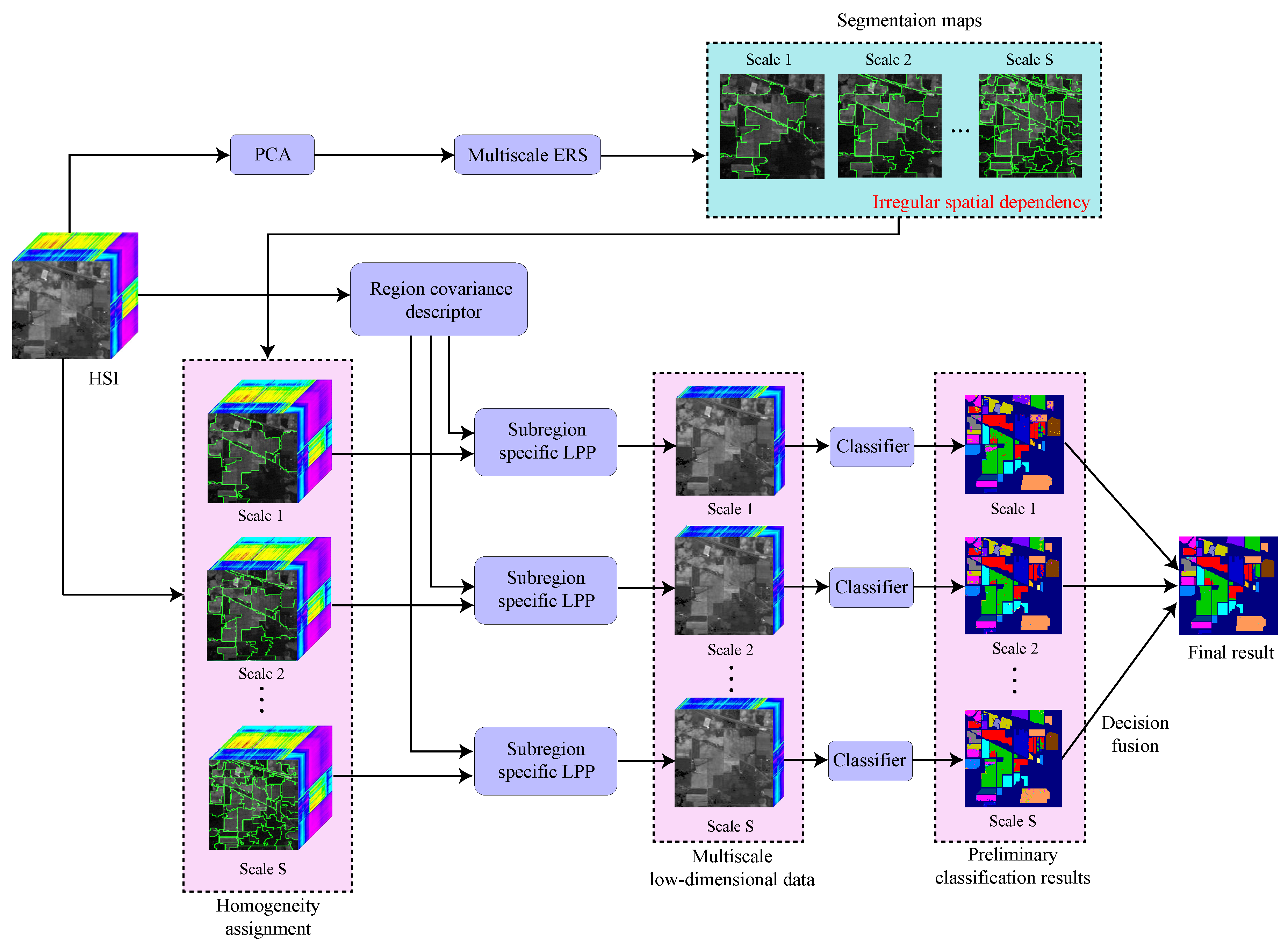
Figure 1. A flowchart of the proposed MSuperLPP for hyperspectral image (HSI) classification.
Applsci 09 02161 g001
Figure 2. Classification accuracy versus training size. (a) Indian Pines with the nearest neighbor classifier. (b) Indian Pines with support vector machine (SVM) classifier. (c) Zaoyuan with nearest neighbor classifier. (d) Zaoyuan with SVM classifier. (e) Salinas with nearest neighbor classifier. (f) Salinas with SVM classifier.
Applsci 09 02161 g002
Figure 3. Classification maps obtained with the Indian Pines data set. (a) Ground truth. (b) GlobalLPP-SF. (c) GlobalLPP-SSCF. (d) SuperLPP-SF. (e) SuperLPP-SSCF. (f) MSuperLPP.
Applsci 09 02161 g003
Figure 4. Classification maps obtained with the Zaoyuan data set. (a) Ground truth. (b) GlobalLPP-SF. (c) GlobalLPP-SSCF. (d) SuperLPP-SF. (e) SuperLPP-SSCF. (f) MSuperLPP.
Applsci 09 02161 g004
Figure 5. Classification maps obtained with the Salinas data set. (a) Ground truth. (b) GlobalLPP-SF. (c) GlobalLPP-SSCF. (d) SuperLPP-SF. (e) SuperLPP-SSCF. (f) MSuperLPP.
Applsci 09 02161 g005
Table 1. The classification accuracy (%) for the Indian Pines data set with the nearest neighbor and SVM classifiers.
Training Size5103050
ClassifierNNSVMNNSVMNNSVMNNSVM
GlobalLPP-SF44.4049.1149.4756.2658.5267.9062.6772.96
GlobalLPP-SSCF62.8163.6568.6768.8777.6677.9980.3980.98
SuperLPP-SF63.7464.1070.7371.6580.9280.3384.0383.14
SuperLPP-SSCF73.5074.3782.2381.3590.4387.9192.2889.38
MSuperLPP76.4975.9185.5383.6094.5593.1097.0295.57
Table 2. The classification accuracy (%) for the Zaoyuan data set with the nearest neighbor and SVM classifiers.
Training Size5103050
ClassifierNNSVMNNSVMNNSVMNNSVM
GlobalLPP-SF64.2675.8171.2981.6477.1884.8479.3486.21
GlobalLPP-SSCF75.1280.1881.0684.9285.7788.5086.6389.19
SuperLPP-SF70.0680.6575.5686.8881.3089.4883.4490.55
SuperLPP-SSCF80.8184.3484.7987.2888.0090.8389.2292.26
MSuperLPP82.2786.6490.1090.6893.8393.7594.4294.39
Table 3. Classification accuracy (%) for the Salinas data set with nearest neighbor and SVM classifiers.
Training Size13510
ClassifierNNSVMNNSVMNNSVMNNSVM
GlobalLPP-SF69.0075.6176.0281.9579.0485.0083.0589.07
GlobalLPP-SSCF78.6980.6085.1486.5587.1188.6989.9791.91
SuperLPP-SF80.6780.5189.8289.3690.7492.0691.9593.32
SuperLPP-SSCF81.7784.2390.9292.3791.9793.2893.8294.50
MSuperLPP90.4688.3295.5594.7396.8796.8997.7897.59