Modeling of a 3D Temperature Field by Integrating a Physics-Specific Model and Spatiotemporal Stochastic Processes


Abstract
1. Introduction
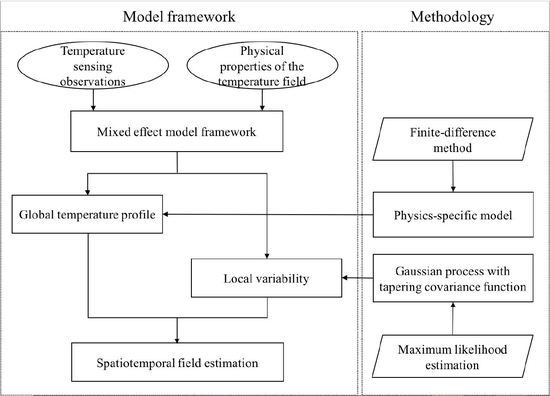
2. Methods
2.1. Formulation
2.2. Physics-Specific Model for the Global Temperature Profile
2.3. Gaussian Process with a Tapering Covariance Function for Local Variability
2.3.1. Formulation of the Gaussian Process Model
2.3.2. Covariance Tapering
2.3.3. Parameter Estimation for θ
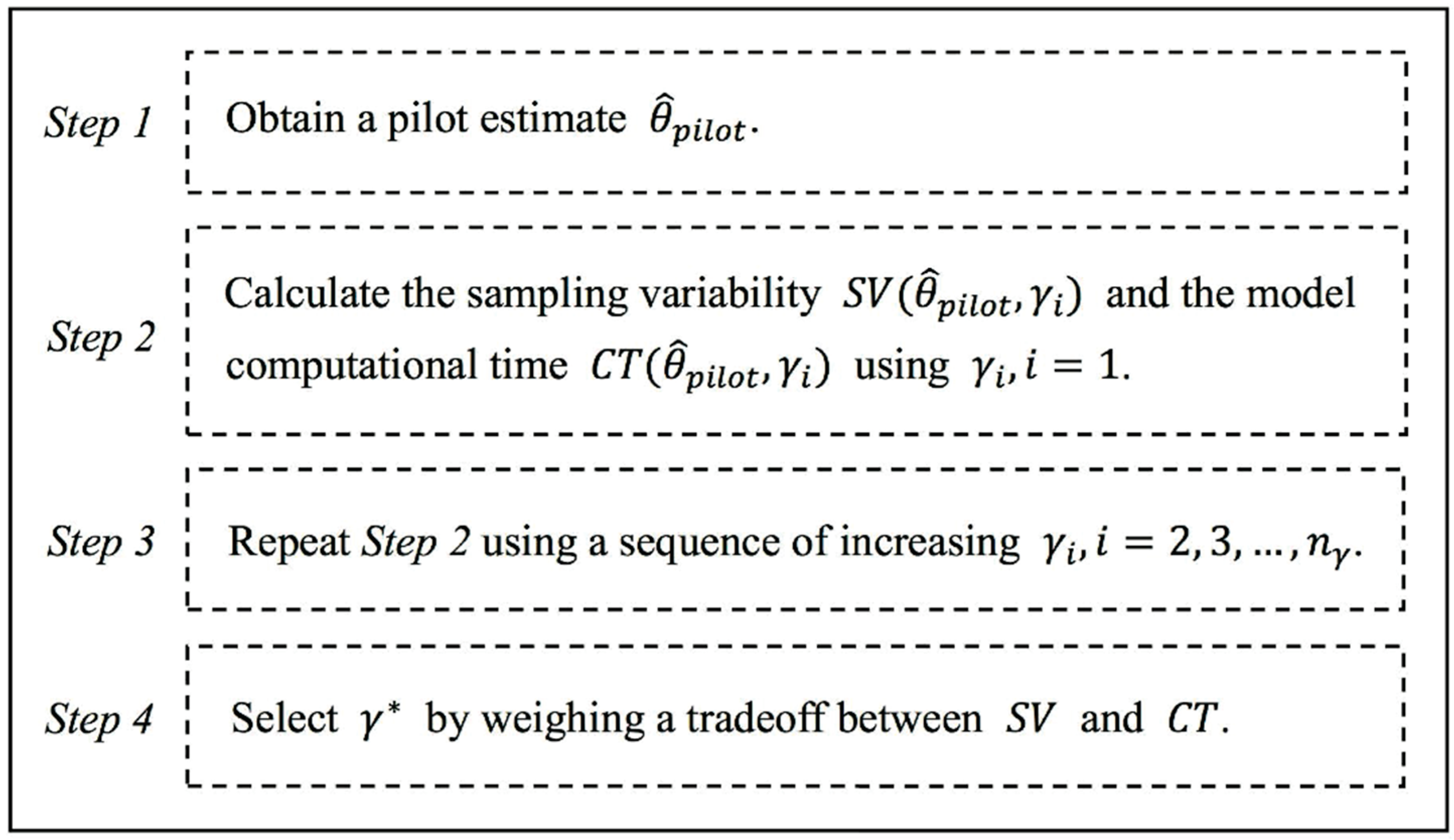
2.3.4. Selection of Range Parameter
2.3.5. Spatiotemporal Field Estimation
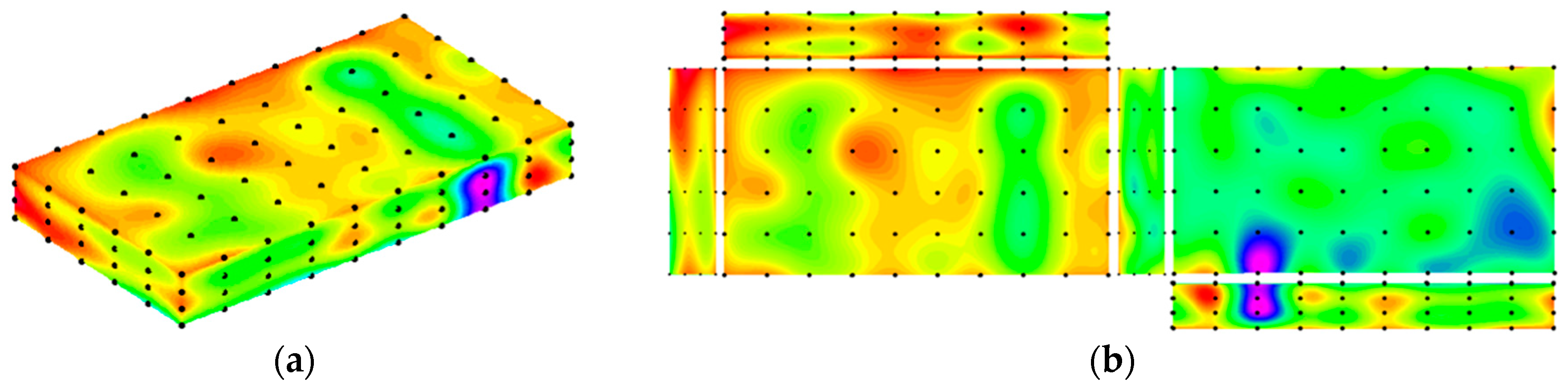
3. Case Study
3.1. Global Temperature Profile
3.2. Parameter Estimation of the Proposed Gaussian Process Model
3.3. Spatiotemporal Field Estimation
4. Conclusions
Author Contributions
Funding
Conflicts of Interest
References
- Zhu, W.; Lü, A.; Jia, S. Estimation of daily maximum and minimum air temperature using MODIS land surface temperature products. Remote Sens. Environ. 2013, 130, 62–73. [Google Scholar] [CrossRef]
- Moser, G.; Serpico, S.B. Automatic parameter optimization for support vector regression for land and sea surface temperature estimation from remote sensing data. IEEE Trans. Geosci. Remote Sens. 2009, 47, 909–921. [Google Scholar] [CrossRef]
- Yao, B.; Yang, H. Physics-driven spatiotemporal regularization for high-dimensional predictive modeling: A novel approach to solve the inverse ECG problem. Sci. Rep. 2016, 6, 39012. [Google Scholar] [CrossRef] [PubMed]
- Chen, Y.; Yang, H. Sparse modeling and recursive prediction of space-time dynamics in stochastic sensor networks. IEEE Trans. Autom. Sci. Eng. 2016, 13, 215–226. [Google Scholar] [CrossRef]
- Zheng, Y.; Liu, F.; Hsieh, H. U-Air: When urban air quality inference meets big data. In Proceedings of the 19th ACM SIGKDD International Conference on Knowledge Discovery and Data Mining, Chicago, IL, USA, 11–14 August 2013; pp. 1436–1444. [Google Scholar]
- Zhou, C.; Wang, K. Spatiotemporal divergence of the warming hiatus over land based on different definitions of mean temperature. Sci. Rep. 2016, 6, 31789. [Google Scholar] [CrossRef] [PubMed]
- Bhandari, S.; Bergmann, N.; Jurdak, R.; Kusy, B. Time series analysis for spatial node selection in environment monitoring sensor networks. Sensors 2018, 18, 11. [Google Scholar] [CrossRef]
- Wang, D.; Zhang, X. A prediction method for interior temperature of grain storage via dynamics model: A simulation study. In Proceedings of the IEEE International Conference on Automation Science and Engineering, Gothenburg, Sweden, 24–28 August 2015; pp. 1477–1483. [Google Scholar]
- Rusinek, R.; Kobylka, R. Experimental study and discrete element method modeling of temperature distributions in rapeseed stored in a model bin. J. Stored Prod. Res. 2014, 59, 254–259. [Google Scholar] [CrossRef]
- Jia, C.; Sun, D.; Cao, C. Finite element prediction of transient temperature distribution in a grain storage bin. J. Agric. Eng. Res. 2000, 76, 323–330. [Google Scholar] [CrossRef]
- Alagusundaram, K.; Jayas, D.S.; White, N.D.G.; Muir, W.E. Three-dimensional, finite element, heat transfer model of temperature distribution in grain storage bins. Trans. ASAE 1990, 33, 577–584. [Google Scholar] [CrossRef]
- Khatchatourian, O.A.; De Oliveira, F.A. Mathematical modeling of airflow and thermal state in large aerated grain storage. Biosyst. Eng. 2006, 95, 159–169. [Google Scholar] [CrossRef]
- Gastón, A.; Abalone, R.; Bartosik, R.E.; Rodriguez, J.C. Mathematical modelling of heat and moisture transfer of wheat stored in plastic bags (silo bags). Biosyst. Eng. 2009, 104, 72–85. [Google Scholar] [CrossRef]
- Jian, F.; Chelladurai, V.; Jayas, D.S.; White, N.D.G. Three-dimensional transient heat, mass and momentum transfer model to predict conditions of canola stored inside silo bags under Canadian Prairie conditions, Part II-model of canola bulk temperature and moisture content. Trans. ASABE 2015, 58, 1135–1144. [Google Scholar]
- Jian, F.; Jayas, D.S.; White, N.D.G.; Alagusundaram, K. A three-dimensional, asymmetric, and transient model to predict grain temperatures in grain storage bins. Trans. ASAE 2005, 48, 263–271. [Google Scholar] [CrossRef]
- Lawrence, J.; Maier, D.E.; Stroshine, L. Three-dimensional transient heat, mass, momentum and species transfer in the stored grain ecosystem: Part I. Model development and evaluation. Trans. ASABE 2013, 56, 179–188. [Google Scholar] [CrossRef]
- Ding, Y.; Elsayed, E.A.; Kumara, S.; Lu, J.; Niu, F.; Shi, J. Distributed sensing for quality and productivity improvements. IEEE Trans. Autom. Sci. Eng. 2006, 3, 344–359. [Google Scholar] [CrossRef]
- Huang, Q.; Rodriguez, K. A software framework for heterogeneous wireless sensor network towards environmental monitoring. Appl. Sci. 2019, 9, 867. [Google Scholar] [CrossRef]
- Li, W.; Zhang, X.; Jia, Y.; Liu, Y. Quality changes of N-3 PUFAs enriched and conventional eggs under different home storage conditions with wireless sensor network. Appl. Sci. 2017, 7, 1151. [Google Scholar] [CrossRef]
- Uchiyama, Y.; Hamatani, T.; Higashino, T. Estimation of core temperature based on a human thermal model using a wearable sensor. In Proceedings of the IEEE 4th Global Conference on Consumer Electronics, Osaka, Japan, 27–30 October 2015; pp. 605–609. [Google Scholar]
- Yin, J.; Wu, Z.; Zhang, Z.; Wu, X.; Wu, W. Comparison and analysis of temperature field reappearance in stored grain of different warehouses. Trans. Chin. Soc. Agric. Eng. 2015, 31, 281–287. [Google Scholar]
- Eisenhower, B.; O’Neill, Z.; Fonoberovand, V.; Mezic, I. Uncertainty and sensitivity decomposition of building energy models. J. Build. Perform. Simul. 2012, 5, 171–184. [Google Scholar] [CrossRef]
- Yang, Y.; Christakos, G.; Huang, W.; Lin, C.; Fu, P.; Mei, Y. Uncertainty assessment of PM2.5 contamination mapping using spatiotemporal sequential indicator simulations and multi-temporal monitoring data. Sci. Rep. 2016, 6, 24335. [Google Scholar] [CrossRef]
- Lermusiaux, P.F.J. Uncertainty estimation and prediction for interdisciplinary ocean dynamics. J. Comput. Phys. 2006, 217, 176–199. [Google Scholar] [CrossRef]
- Sapsis, T.P.; Lermusiaux, P.F.J. Dynamically orthogonal field equations for continuous stochastic dynamical systems. Phys. D Nonlinear Phenom. 2009, 238, 2347–2360. [Google Scholar] [CrossRef]
- Rasmussen, C.E. Gaussian Processes in Machine Learning in Advanced Lectures on Machine Learning; Springer: Berlin/Heidelberg, Germany, 2004; pp. 63–71. [Google Scholar]
- Krause, A.; Singh, A.; Guestrin, C. Near-optimal sensor placements in Gaussian processes: Theory, efficient algorithms and empirical studies. J. Mach. Learn. Res. 2008, 9, 235–284. [Google Scholar]
- Sang, H.; Huang, J.Z. A full-scale approximation of covariance functions for large spatial data sets. J. R. Stat. Soc. Ser. B (Stat. Methodol.) 2012, 74, 111–132. [Google Scholar] [CrossRef]
- Cressie, N.; Wikle, C.K. Statistics for Spatio-Temporal Data; John Wiley and Sons: Hoboken, NJ, USA, 2015. [Google Scholar]
- Xun, X.; Cao, J.; Mallick, A.; Maity, A.; Carroll, R.J. Parameter estimation of partial differential equation models. J. Am. Stat. Assoc. 2013, 108, 1009–1020. [Google Scholar] [CrossRef]
- Bland, D.R. Solutions of Laplace’s Equation; Springer Science and Business Media: Berlin/Heidelberg, Germany, 2012. [Google Scholar]
- Zhang, B.; Sang, H.; Huang, J.Z.; Maity, A.; Carroll, R.J. Full-scale approximations of spatio-temporal covariance models for large datasets. Stat. Sin. 2015, 25, 99–114. [Google Scholar] [CrossRef][Green Version]
- Kaufman, G.G.; Schercish, J.M.; Nychka, D.W. Covariance tapering for likelihood-based estimation in large spatial data sets. J. Am. Stat. Assoc. 2008, 103, 1545–1555. [Google Scholar] [CrossRef]
- Yang, Z. A simulation of the quasi-static temperature field in grain storage via CFD. J. Chin. Cereals Oils Assoc. 2010, 25, 46–50. [Google Scholar]


| Material | |
|---|---|
| Mixed wheat | 5.56, 5.55, 1.50 |
| 0.1289 | 10.4956 | 10.1552 | 2.9974 | 0.0154 |
| Model | MSE |
|---|---|
| Constant + Gaussian process with tapering covariance function | 7.86 |
| Sinusoidal model + Gaussian process with tapering covariance function | 0.60 |
| Thermodynamic model + Gaussian process with tapering covariance function | 0.04 |
| Model | MSE | Computational Time/s |
|---|---|---|
| Thermodynamic model | 0.45 | - |
| Thermodynamic model + conventional Gaussian process | 0.04 | 129.23 |
| Thermodynamic model + Gaussian process with tapering covariance function | 0.04 | 63.81 |
© 2019 by the authors. Licensee MDPI, Basel, Switzerland. This article is an open access article distributed under the terms and conditions of the Creative Commons Attribution (CC BY) license (http://creativecommons.org/licenses/by/4.0/).
Share and Cite
Wang, D.; Zhang, X. Modeling of a 3D Temperature Field by Integrating a Physics-Specific Model and Spatiotemporal Stochastic Processes. Appl. Sci. 2019, 9, 2108. https://doi.org/10.3390/app9102108
Wang D, Zhang X. Modeling of a 3D Temperature Field by Integrating a Physics-Specific Model and Spatiotemporal Stochastic Processes. Applied Sciences. 2019; 9(10):2108. https://doi.org/10.3390/app9102108
Chicago/Turabian StyleWang, Di, and Xi Zhang. 2019. "Modeling of a 3D Temperature Field by Integrating a Physics-Specific Model and Spatiotemporal Stochastic Processes" Applied Sciences 9, no. 10: 2108. https://doi.org/10.3390/app9102108
APA StyleWang, D., & Zhang, X. (2019). Modeling of a 3D Temperature Field by Integrating a Physics-Specific Model and Spatiotemporal Stochastic Processes. Applied Sciences, 9(10), 2108. https://doi.org/10.3390/app9102108