Improved Probability Prediction Method Research for Photovoltaic Power Output

Abstract

Due to solar radiation and other meteorological factors, photovoltaic (PV) output is intermittent and random. Accurate and reliable photovoltaic power prediction can improve the stability and safety of grid operation. Compared to solar power point prediction, probabilistic prediction methods can provide more information about potential uncertainty. Therefore, this paper first proposes two kinds of photovoltaic output probability prediction models, which are improved sparse Gaussian process regression model (IMSPGP), and improved least squares support vector machine error prediction model (IMLSSVM). In order to make full use of the advantages of the different models, this paper proposes a combined forecasting method with divided-interval and variable weights, which divides one day into four intervals. The models are combined by the optimal combination method in each interval. The simulation results show that IMSPGP and IMLSSVM have better prediction accuracy than the original models, and the combination model obtained by the combination method proposed in this paper further improves the prediction performance.

1. Introduction

At present, the average natural gas storage in the world is 53 years. There is more coal in storage than oil and natural gas, and the world’s coal storage capacity is 15,980 tons, which can be mined for about 200 years [1]. It can be seen that a shortage of fossil fuels is imminent. Photovoltaic (PV) power generation has developed rapidly in the world in recent years due to its advantages in meeting energy demands, reducing environmental pollution, and improving energy structure [2]. As a result of solar radiation and other factors, PV power output has high volatility and randomness, and with the increase of photovoltaic grid-connected capacity, this adverse impact will bring more and more risks to grid operation. Therefore, accurate prediction of photovoltaic power generation will be of great significance to the stability and safety of grid dispatching and power systems [3].

In many previous studies, the prediction of photovoltaic power generation based on physical models has shown great progress. Zhang et al. [4] established the basic model of the photovoltaic cell and photoelectric conversion efficiency based on the principle of photovoltaic power generation and photoelectric conversion efficiency model. Then empirical formulas affecting photoelectric conversion efficiency were obtained, and reasonable empirical parameters were selected to predict PV output power. Dolara et al. [5] proposed the three-parameter, four-parameter, and five-parameter equivalent circuit model comparison method for photovoltaic cells and two thermal models for estimating battery temperature, which can achieve better accuracy with fewer parameter solutions. However, the creation of physical model and parameter solving process are complicated, and the anti-interference ability of the model is poor.

With the development of machine learning technology and computer hardware capabilities, an increasing number of machine learning and statistical regression methods have been applied to the field of photovoltaic power generation prediction. This includes artificial neural network algorithms [6], support vector machine (SVM) algorithms [7,8], the ARMAX algorithm [9], the Markov chain algorithm [10], and so on. Chen et al. [11] proposed a neural network-based photovoltaic power generation prediction model that can predict power generation under different weather conditions one day in advance. Chen et al. [12] proposed a solar irradiance prediction method based on the support vector machine algorithm. This method uses different kernel functions to predict solar irradiance, which are then compared. Based on the ARMAX algorithm, Li et al. [13] considered meteorological factors to obtain more-accurate prediction results. A photovoltaic power generation prediction model based on an improved Markov chain was proposed by Ding [14]. The Markov chain is mainly used to correct the residual of the prediction model to improve accuracy. However, these algorithms have obvious defects. It is easy for the neural network algorithm to fall into the local minimum, and the model is not well explained. The support vector machine has limited processing ability for large samples of data, and the time series method has weak non-stationary processing ability. Many scholars have improved the efficiency of models by improving the algorithm. Eseye et al. [15] used the particle swarm optimization (PSO) to optimize the normalization parameters and kernel parameters of SVM. The back propagation (BP) neural network algorithm was improved by combining the momentum term with the variable learning rate, so the defects—the traditional BP learning algorithm is liable to fall into local minimum points, and has a slow convergence rate—were remedied. The improved BP neural network is used to improve the predictive performance [16].

The output of PV generation is restricted by its external environment, and the weather has a greater impact on photovoltaic systems. In order to reduce the impact of weather, data are classified according to the type of the weather. Some results prove that such methods have a better performance [17,18]. In most models, only conventional variables such as temperature, humidity, and wind speed are generally considered, so the accuracy of these models will decrease under extreme weather conditions. The aerosol index (AI) can indicate that there is a strong linear relationship between particulate matter in the atmosphere and solar radiation attenuation, which has a potential impact on the energy generated by photovoltaic panels. In [19], based on the classification of seasons, AI can be used as an additional input parameter to adapt to the complicated environment. The drawback of these methods, then, is that the accuracy of models depends largely on the accuracy of the weather classification.

The accuracy of predictive models based on statistical learning depends mainly on a large amount of historical data. However, historical data contains complex information, and there is redundant information that may not be necessary. Not all weather factors have a significant impact on PV output, so we need to extract or remove information from historical data to reduce the complexity of models. In [20], it is shown that temperature and insolation are positively correlated with PV power, humidity is negatively correlated with PV power, and wind speed has no obvious correlation with PV power by the correlation analysis. Therefore, air temperature, humidity, insolation, and historical PV power can be selected as inputs to the prediction model to reduce the complexity of the data. Zhu et al. [21] proposed a PV output prediction method combining wavelet decomposition and the artificial neural network (ANN) algorithm. After separating the useful information and the interference information by wavelet decomposition, the neural network model is used to obtain the predicted power value. Malvoni et al. [22] combined the quadratic Renyi entropy criteria with principal component analysis (PCA) to reasonably reduce the data dimension and use least squares support vector machines (LSSVM) to predict future PV power. This model can facilitate calculation, while improving accuracy. In addition, it has been found that the introduction of image data can also improve prediction accuracy. Marquez et al. [23] proposed a method for combining solar cloud image data and artificial neural network models to predict solar irradiance. Zhu Xiang et al. [24] used cloud information and cloud maps in numerical weather prediction (NWP) to predict the power attenuation caused by cloud clusters blocking photovoltaic power plants over the subsequent 4 hours, then corrected the predicted values to improve the accuracy of model prediction. This type of method requires more advanced experimental equipment, however.

Most of the research has aimed to predict a certain value at a certain moment, but it is difficult for point prediction values to express the uncertainty of the prediction result, which will affect power grid scheduling and the stability of the power system. Compared with point prediction, probabilistic prediction makes up for the shortcoming that point prediction cannot measure the uncertainty of prediction results [25]. Due to the uncertainty of solar resources and the inherent defects of the prediction model, the point prediction error of solar power cannot be avoided, and the defect that the point prediction result cannot make a quantitative description of the uncertainty of solar power is difficult to overcome. In terms of the application of solar power, there needs to be a relatively accurate estimation of the fluctuation range of solar power, which requires planning, operation, safety, and stability analysis of the power grid (including solar power generation). The probabilistic prediction of solar power generation expands the connotations of solar power generation prediction, and can provide the probability distribution of PV power generation. The diversity of probability distribution at different time points can provide power system policymakers with an abundance of uncertain information, including economic dispatch, rotating standby arrangement, and electricity market price optimization problems. In a word, the probabilistic prediction method can give the possible PV power value and its probability distribution in the next moment, and provide more-comprehensive prediction information [26]. However, the current research on probability prediction in the field of photovoltaic power generation is still in its infancy. Fatemi et al. [27] proposed two parametric probability prediction methods for predicting solar irradiance by β-distribution and bilateral power distribution, effectively predicting solar irradiance and accurately describing its stochastic characteristics. Fonseca et al. [28] assumed the prediction error distribution as the normal distribution and the Laplacian distribution. The probability distribution of the generated power and the confidence interval value at different confidence levels was then obtained by the maximum likelihood estimation method. Almeida et al. [29] used the meteorological data obtained by NWP as input data, and a probability prediction model based on a quantile regression prediction algorithm was established to study the probability prediction of photovoltaic power generation. Mohammad et al. [30] combined the probability distribution theory with the Gaussian mixture method, and the prediction results are consistent with the actual probability distribution of photovoltaic power under different weather conditions.

Considering that PV output is affected by many weather factors, and that the complexity of a model will increase if too many variables exist, this paper preprocesses the original data set based on feature selection and similar sample classifications. It is difficult for the point prediction method to express the uncertainty of prediction results. Two improved photovoltaic power generation probabilistic prediction models are proposed in this paper to improve the preliminary prediction performance. The idea of traditional combination methods is to combine different algorithms to optimize a certain prediction model without changing the essential structure of the models. Through analysis, it was found that different models had different advantages during different periods of time. In order to improve the prediction accuracy by contributing to the advantages of the different models, a new probability prediction model with multi-interval and variable weight is proposed. The method is applied to handle the uncertainties of photovoltaic power generation for the first time, to the best of our knowledge.

The major contributions and innovations of this paper are as follows:

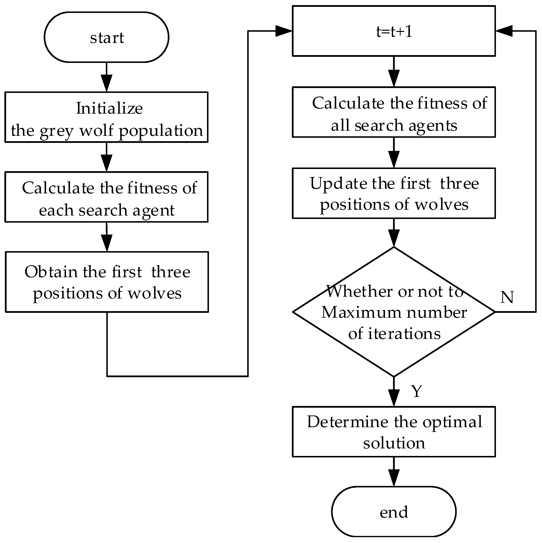
1. The improved grey wolf optimization algorithm is used to optimize the sparse Gaussian process model and the least squares support vector machine model. The better super-parameter values are obtained, which improve accuracy.

2. An error correction probability prediction model based on improved least squares support vector machine (IMLSSVM) is proposed. The model can be corrected by using the historical error distribution to realize the probability prediction model under the premise of realizing point prediction.

3. A piecewise optimal combination model is proposed that uses different combined weighting coefficients in different periods to make full use of different prediction models.

2. Single Improved Prediction Model

In this part, two improved prediction models will be introduced. The Gaussian process (GP) is a generalization of the Gaussian probability distribution. The sparse Gaussian process regression (SPGP) model is a supervised learning model based on Bayesian theory and statistical theory. Least squares support vector machine (LSSVM) is a machine learning algorithm based on statistical learning theory. In order to obtain the optimal solution of the super-parameters, the improved grey wolf optimization algorithm was used to solve the super-parameters of the SPGP model and LSSVM. In this paper, improved SPGP model and LSSVM model are used to predict photovoltaic power, respectively.

2.1. Improved Sparse Gaussian Process Regression Model

2.1.1. Sparse Gaussian Process Regression

In the Gaussian process (GP) [31] model, it is assumed that the prior distribution of the observed values is $y$ given by a Gaussian whose mean is zero and whose covariance is defined by a Gram matrix $K+{\sigma }_n^{2}I$ so that

$$y~N(0,K+{\sigma }_n^{2}I)$$

(1)

where K = k(x_n,x_n) with k as the kernel function. For a new input $X_{*}$, a prediction of the target variable $f_{*}$ can be made by using the rules for conditioning Gaussians. The predictive distribution $f_{*}$ is a Gaussian distribution with mean $\overline{f_{*}}$ and covariance $\mathrm{cov}(f_{*})$. The posterior distribution of the predicted values is

$$f_{*}|X,y,X_{*}~N(\overline{f_{*}},\mathrm{cov}(f_{*}))$$

(2)

where $\overline{f_{*}}=E[f_{*}|X,y,X]=K(X_{*},X){[K(X,X)+{\sigma }_n^{2}I]}^{-1}y,\mathrm{cov}(f_{*})={\sigma }_n^2+K(X_{*},X_{*})-K(X_{*},X){[K(X,X)+{\sigma }_n^{2}I]}^{-1}\ast K(X,X_{*})$.

In this paper, the commonly used automatic relevance determination function is chosen as the covariance function.

$$k(x_p,x_q)={\sigma }_f^2\exp (-\frac{1}{2l^2}{\Vert x_p-x_q\Vert }^2)+{\sigma }_n^2{\delta }_{pq}$$

(3)

where x_p, x_q are the variables of training or test sets, l, σ_f, σ_n are the hyper-parameters, and δ_pq is the symbolic function.

A main drawback of GP is its high time complexity. A training process requires inverting a matrix K+σ_n²I, which costs O(n³). In order to solve this problem, in this paper, an SPGP model that adopts the fully independent training conditional approximation (FITC) approximation method [32] is introduced. The FITC method adopts a pseudo dataset D and uses M samples to approximately simulate the original dataset, where the number of samples M << N. So the posterior distribution $\overline{f}$ over pseudo targets $\overline{X}$ can be obtained.

$$p(\overline{f}|D,\overline{X})=N(K_M{Q}_M^{-1}{K}_{MN}{(\mathsf{\Lambda }+{\sigma }^{2}I)}^{-1}y,K_M{Q}_M^{-1}{K}_M)$$

(4)

where ${[K_M]}_{m{m}^{’}}=K({\overline{x}}_m,{\overline{x}}_{m^{’}})$, $Q_M=K_M+K_{MN}{(\mathsf{\Lambda }+{\sigma }^{2}I)}^{-1}{K}_{NM}$, ${[K_{MN}]}_{mn}=K(x_m,{\overline{x}}_n)$, and $\mathsf{\Lambda }=diag(\mathsf{\lambda }),{\lambda }_n=K_{nn}-k_n^{\top }{K}_M^{-1}{k}_n$. Finally, predictive distribution of test data $y_{*}$ can be obtained and it is a Gaussian distribution with mean ${\mu }_{*}$ and covariance ${\sigma }_{*}^2$.

$$p(y_{*}|x_{*},D,\overline{X})={\displaystyle \int p(\overline{f}|D,\overline{X})}p(y_{*}|x_{*},\overline{X},\overline{f})\mathrm{d}\overline{f}=N({\mu }_{*},{\sigma }_{*}^2)$$

(5)

where ${\mu }_{*}=k_{*}^{\top }{Q}_M^{-1}{K}_{MN}{(\mathsf{\Lambda }+{\sigma }^{2}I)}^{-1}y,{\sigma }_{*}^2=K_{**}-k_x^{\top }(K_M^{-1}-Q_M^{-1})k_{*}+{\sigma }^2,{\sigma }_{*}^2=K_{**}-k_x^{\top }(K_M^{-1}-Q_M^{-1})k_{*}+{\sigma }^2$.

The matrix $K_{MN}{(\mathsf{\Lambda }+{\sigma }^{2}I)}^{-1}{K}_{NM}$ is O(M²N). Since M is much less than N, the computational costs are lower than those of the GP.

2.1.2. Improved Grey Wolf Optimization Algorithm

Because the SPGP model is complicated and the concavity and convexity of the optimization problem formula (Equation (7) cannot be judged intuitively, traditional convex optimization methods may not be applicable to the solution of the hyper-parameter in the SPGP model. Moreover, because this method relies too heavily on initial values, it falls easily into local optimum. Therefore, this paper introduces an improved grey wolf optimization algorithm to optimize the hyper-parameter. Grey wolf optimization (GWO) is a heuristic population intelligent optimization algorithm proposed by Mirjalili in 2014 [33]. It has the advantages of simple principles, less parameters and a strong global search ability, but there is still much room for improvement in the algorithm.

When dealing with the optimization problem, it is assumed that in the D-dimensional search space, the number of grey wolves is N, and the position of the i-th wolf is defined as $X_i=(X_i^1,\cdots ,X_i^D)$, where $X_i^k$ indicates the position of the i-th wolf in the k-th dimension. This paper will improve the algorithm to obtain an improved grey wolf optimization (IMGWO) according to the following three aspects:

(1) Opposition-based learning algorithm: The initial population is obtained by randomly generated methods in the GWO algorithm. However, the initial population will affect the search efficiency and the quality of the solution. Therefore, this paper adopts the method of opposition-based learning to generate a diverse initial population. Assuming that there is a number x in [m, n], the opposite point of x is defined as x’ = m+n−x.

(2) Nonlinear convergence factor: A common problem facing optimization algorithms is how to balance a global search ability with a local search ability. In GWO, the convergence factor decreases linearly from 2 to 0 over the course of iterations. It cannot reflect the actual search process because the process is not linear. Therefore, in this paper, a new non-linear convergence factor is proposed: $\overrightarrow{a}=2-2(k/K){)}^n$, where k indicates the current iteration, K is the maximum number of iterations, n is the attenuation order, and n is 3.

(3) Dynamic weight updating: In the stage of position updating, GWO uses an equal weight method that ignores the different characteristics of alpha, beta, and delta. The wolves have different importance for the population, so we need different weights to reflect the different importance. In this paper, fitness values are used to describe the importance of wolves. Equation (6) is adopted to update location information:

$$\overrightarrow{X}(t+1)=w_{\alpha }{\overrightarrow{X}}_1+w_{\beta }{\overrightarrow{X}}_2+w_{\sigma }{\overrightarrow{X}}_3$$

(6)

where $w_i=f(X_i(t))/(f(X_{\alpha }(t))+f(X_{\beta }(t))+f(X_{\delta }(t)))(i=\alpha ,\beta ,\delta )$ is the weight coefficient, $f(X_i(t))$ is the fitness value, and ${\overrightarrow{X}}_i(i=\alpha ,\beta ,\delta )$ is the position of the wolf.

In this paper, the flow chart of the GWO algorithm is given, as shown in Figure 1.

The main difficulty of SPGP lies in the solution of the hyper-parameters. In order to obtain the hyper-parameters, this paper adopts the sum of root mean square error (RMSE) and continuous ranking probability score (CRPS) as a target fitness. The fitness is shown as:

$$\{\begin{array}{c}\min (RMSE+CRPS)\\ s.t.0\le RMSE\le 1\\ 0\le CRPS\le 1\end{array}$$

(7)

2.2. Improved Least Squares Support Vector Machine Error Prediction Model

2.2.1. Improved Least Squares Support Vector Machine

Because of the quadratic programming problem under the constraint of inequality in the support vector machine, the calculation amount is large. In order to improve the calculation speed, Vandewallw et al. [34] proposed LSSVM in 1999, and converted the inequality constraint into an equality constraint. The complex convex quadratic programming problem is transformed into a linear equation solution. Its optimization objective function is as follows:

$$\begin{array}{l}\min \{\frac{1}{2}w\cdot w+\frac{C}{2}{\displaystyle \sum _{i=1}^n{\epsilon }_i^2}\}\\ s.t.\hspace{1em}{y}_i=w\cdot \phi (x_i)+b+{\epsilon }_i,i=1,2\cdots ,n\end{array}$$

(8)

where $w$ is the weight coefficient vector, C and b are constants, and ${\epsilon }_i$ is the error.

In order to solve the minimization problem, the Lagrangian function method is used.

$$L(w,b,{\epsilon }_i,\alpha )=\frac{1}{2}w\cdot w+\frac{C}{2}{\displaystyle \sum _{i=1}^n{\epsilon }_i^2}-{\displaystyle \sum _{i=1}^n{\alpha }_i[w\cdot \phi (x_i)+b+{\epsilon }_i-y_i]}$$

(9)

where $\alpha$ is Lagrangian factor.

Then we need to take the derivative of these parameters:

$$\begin{array}{l}\frac{\partial L}{\partial w}=w-{\displaystyle \sum _{i=1}^n{\alpha }_i\phi (x_i)}=0\hfill \\ \frac{\partial L}{\partial b}={\displaystyle \sum _{i=1}^n{\alpha }_i=0}\hfill \\ \frac{\partial L}{\partial {\epsilon }_i}=C{\epsilon }_i-{\alpha }_i=0\hfill \\ \frac{\partial L}{\partial {\alpha }_i}=w\cdot \phi (x_i)+b+{\epsilon }_i-y_i=0\hfill \end{array}$$

(10)

The LSSVM model can be obtained by solving the above equation, which can be expressed as

$$f(x)={\displaystyle \sum _{i=1}^n{\alpha }_{i}K(x_i,x)+b}$$

(11)

where $K(x_i,x)$ is the kernel function.

This paper implements the optimization process of the LSSVM using the IMGWO algorithm.

2.2.2. Error Probability Distribution of Power Prediction

If the potential law of the prediction error can be properly expressed, then the prediction value can be corrected to improve the prediction performance. In this paper, the prediction values are obtained via LSSVM, and the corresponding prediction error values are be obtained by calculation. The methods for estimating the distribution of error can be divided into parameter estimation and non-parametric estimation. The parameter estimation assumes that the data sample obeys a known distribution function, and that the samples are used to estimate the parameter values of the distribution function. Normal distribution, T-location-scale distribution, and logistic distribution are the distribution functions commonly used. Non-parametric estimation is based on the characteristics of the sample data, not a priori estimation of data samples. The entire estimation process is completely driven by the data samples, and has a strong utility to the problem which is impossible to estimate the characteristics of its sample data in advance. Kernel density estimation (KDE) [35] is chosen as the nonparametric estimation method in this paper. $X_1,X_2,\cdots ,X_n$ is the overall sample, and $x_1,x_2,\cdots ,x_n$ represents the observed values of samples. The kernel density estimate of the probability density function at any point x is defined as

$$f_h(x)=\frac{1}{nh}{\displaystyle \sum _{i=1}^{n}K(\frac{x-X_i}{h})}$$

(12)

where f_h(x) is the estimated probability density function, h is the window width, and $K(\cdot )$ is the kernel function.

Through statistical analysis of the error between the actual and predicted values of photovoltaic power generation, we find that the prediction errors in different power intervals have different distributions, which is quite different from the distribution of the overall prediction error. Therefore, this paper divides the data into multiple intervals, and performs statistical analysis on the error of each interval to calculate the probability density function. When the sample data is relatively sufficient, the empirical distribution is similar to the overall distribution, and it can be treated as the total distribution.

For the division of intervals, there are no fixed rules to follow. If the number of the intervals is too large, the amount of sample data in each interval will be small. The empirical distribution will be different from the overall distribution, which cannot reflect the real information of sample data. On the contrary, the intrinsic information and the meaning of segmentation statistics will be lost. Assuming that the length of the interval is $\Delta P$ and the power interval range is $[P_1,P]$, the power is divided at equal intervals.

$$D_i=[P_1+(i-1)\Delta P,P_1+i\Delta P]$$

(13)

where $i=1,\cdots ,N$, and N is the number of intervals.

By dividing the range of each interval by Equation (13), there may be cases where the number of samples in some intervals is too small. In order to better reflect the distribution of data, it is necessary to adjust the range of the interval to a certain extent, according to the actual situation.

3. Probability Prediction Combination Model

The essence of the combination method is to find the respective superior information in a variety of models that can more fully describe the sample information than single model. Therefore, it, with a stronger anti-interference ability, can effectively reduce the influence of complex environmental factors [36]. It should be noted that the performance of any single model directly effects the accuracy of the combined model. Considering the calculation cost and effect comprehensively, the number of single models is often taken as two to five. In addition, the quantile regression neural network (QRNN) model has better performance in predicting PV output [37]. This model and the proposed two improved models will be used to construct the combined model in this paper. In this part, a piecewise optimal combination model is proposed that uses different combined weighting coefficients in different periods to make full use of different prediction models.

3.1. Optimal Combination Method

The optimal combination method is based on the functional relationship between the combination model and the single model. The objective function is constructed under certain constraints, and the weight coefficient of the single models in the combination method is solved by maximizing the objective function.

The non-optimal combination method mainly follows the simple and convenient principle of obtaining the weight coefficient using methods such as the arithmetic average method, the root mean square error reciprocal method, the entropy method, and so on. The accuracy of the non-optimal combination method is generally lower than that of the optimal combination method. In this paper, the interpretation of the optimal linear combination method is given by taking the sum of squared prediction errors as the objective function to solve the weight coefficient.

If x_t is the true value of the t-th sample, x_it is the predicted value of the t-th sample in the i-th single model, and e_it is the error value of the t-th sample of in the i-th prediction model, then $e_{it}=x_t-x_{it}$. In order to ensure the validity and unbiasedness of the results, the weight coefficient needs to meet the following conditions:

$${\displaystyle \sum _{i=1}^m{w}_i}=1$$

(14)

where $w_i$ represents the weight coefficient of the i-th single model. The sum of the squared error of the combination model can be expressed as follows:

$$J={\displaystyle \sum _{t=1}^n{e}_t^2}={\displaystyle \sum _{t=1}^n{\displaystyle \sum _{i=1}^m{\displaystyle \sum _{j=1}^{m}w{}_{i}e{}_{it}w{}_{j}e{}_{jt}}}}$$

(15)

Therefore, the linear combination model can use the sum of the squared error as the objective function. If $W={(w_1,\cdots ,w_m)}^T,E_{ij}=e_i^T{e}_j={\displaystyle \sum _{i=1}^N{e}_{it}{e}_{jt}},E={(E_{ij})}_{n\times n}$, R is an n-dimensional column vector where each element is 1, and E is a square matrix of $n\times n$, which represents the information matrix of the combined prediction error, then the solution of the weight coefficient can be expressed as an optimization problem.

$$\begin{array}{c}\min J={\displaystyle \sum _{t=1}^n{e}_t^2}=L^{T}EL\hfill \\ s.t.\hspace{1em}{R}^{T}L=1\hfill \\ L\ge 0\end{array}$$

(16)

The solution is described in detail in [38]. For the solution of the weight coefficient in the optimal combination, this paper uses the IMGWO proposed in this paper to solve the problem. The position of wolves is the value of the weight coefficient.

3.2. Combination Method with Variable Intervals and Weights

In order to fully utilize the characteristics of each model at different time periods, a combination method with different weights of intervals is proposed. For example, the accuracy of method A at interval 1 is higher than that of method B, and the prediction accuracy at interval 2 is lower than that of method B, so method A and method B will have different weight coefficients in different time intervals.

When the day is divided into H intervals, the corresponding combination model will be respectively established. In this paper, the daily time period is divided into four intervals. Interval I is from 06:00 to 09:00, interval II is from 09:00 to 12:00, interval III is from 12:00 to 15:00, and interval IV is from 15:00 to 18:00. In the actual experiment, we first need to determine which time interval the predicted data belongs to, then use the combination model to predict the power generation. In this paper, a flow chart of the combination method is given, shown in Figure 2.

4. Experiment

4.1. Data Preprocessing

The dataset used in this paper is acquired from solar power station, from 2012 to 2014, of the Energy Forecasting Working Group of the Institute of Electrical and Electronics Engineers, including the 24-hour PV output value of photovoltaic panels and corresponding meteorological parameters such as surface solar irradiance, atmosphere, irradiance, surface pressure, total cloud amount, and so on [39]. Since the output of the photovoltaic panel was 0 at night, the data from 6:00 to 18:00 every day is selected as the raw data.

$${\overline{x}}_{ij}=\frac{x_{ij}-x_{\min ,\mathrm{j}}}{x_{\max ,\mathrm{j}}-x_{\min ,\mathrm{j}}}$$

(17)

where $x_{ij}$ is the i-th data of the j-th variable in the original dataset; $x_{\min ,\mathrm{j}}$ and $x_{\max ,\mathrm{j}}$ are the minimum and maximum values of the j-th variable in the original dataset, respectively; and ${\overline{x}}_{ij}$ is the i-th new data of the j-th variable after the normalization. The target variable values were normalized by the Energy Forecasting Working Group, so its rang is [0,1]. The other 12 variables provided were not normalized, and had different dimensions. After the normalization, the range of 12 variables are all [0,1].

If all variables are considered, it will inevitably increase the model complexity and training time. The random forest algorithm can solve the high-dimensional data classification and regression problem [40,41]. This paper uses the algorithm to select the variables affecting the PV output value. The variable description and processing results are shown in

Table 1. Variable description.

Name	Unit	Score
Total column liquid water (TCLW)	kg·m−2	13.2
Total column ice water (TCIW)	kg·m−2	19.4
Surface pressure (SP)	Pa	15.1
Relative humidity at 1000 mbar (RH)	%	62.6
Total cloud cover (TCC)	0–1	16.8
10 meter U wind component (10 U)	m·s−1	21.7
10 meter V wind component (10 V)	m·s−1	13.3
2 meter temperature (2T)	K	39.7
Surface solar rad down (SSRD)	J·m−2	370.3
Surface thermal rad down (STRD)	J·m−2	50.7
Top net solar rad (TSR)	J·m−2	208.0
Total precipitation (TP)	M	11.4

.

The 12 variables obtained from the European Centre for Medium-Range Weather Forecasts (ECMWF) NWP output are independent. Total column liquid water (TCLW) represents the vertical integration of cloudy liquid water content. Relative humidity at 1000 mbar (RH) is defined with respect to the saturation of the mixed phase (i.e., with respect to saturation over ice below −23 °C, and with respect to saturation over water above 0 °C). Total cloud cover (TCC) is derived from model levels using the model’s overlap assumption. Top net solar rad (TSR) is the net solar radiation at the top of the atmosphere. Surface solar rad down (SSRD), surface thermal rad down (STRD), top net solar rad (TSR), and total precipitation (TP) are all accumulated data.

The importance scores of 12 meteorological parameters can be obtained by the random forest algorithm. The importance scores of the meteorological factors are shown from Table 1, and the importance ranking is performed according to the scores of the respective variables. A variable is more important when its score is higher. If there are too few variable factors left in the feature selection process, important information may be lost and the prediction accuracy may be affected. Therefore, the first six feature variables are selected as the input variables set through many tests. The six variables are SSRD, TSR, RH, STRD, 2T, 10U.

The photovoltaic power generation will show different trends under different weather conditions, and the prediction accuracy will be improved by classifying the original data and selecting similar sample. A fuzzy clustering algorithm can deal with similarity and fuzzy relations, so the algorithm is used to further process the data. On the one hand, too many classification types will make the number of samples for each type too small. On the other hand, PV output usually shows instability in the case of bad weather such as rainy days. The data are divided into sunny and rainy days by a fuzzy C-means clustering algorithm. The algorithm theory and calculation process are described in [20].

4.2. Evaluation Criteria

This paper introduces the evaluation criteria of point prediction value and confidence interval prediction value, which can evaluate the prediction probability distribution performance.

1) The root mean square error is defined as follows:

$$RMSE=\sqrt{\frac{{\displaystyle \sum _{i=1}^N{(y_i-y_i^{\prime })}^2}}{N}}$$

(18)

where N indicates the number of test set data, and $y_i$ and $y_i^{\prime }$ represent the i-th predicted value and the actual value, respectively. The smaller the root mean square error value is, the higher the prediction accuracy of the model.

2) The continuous ranking probability score is a comprehensive criterion for evaluating probability prediction performance. It can simultaneously evaluate the calibration degree and sharpness of the probability distribution. The smaller the value is, the better the prediction effect of the model will get. CRPS is defined as follows:

$$CRPS(F,x)=\{\begin{array}{l}{\displaystyle \underset{-\infty }{\overset{\infty }{\int }}{\{F(y)-1\}}^{2}dy},y\ge x\\ {\displaystyle \underset{-\infty }{\overset{\infty }{\int }}{(F(y))}^{2}dy},y<x\end{array}$$

(19)

where x is the actual observed value and F is the predicted cumulative distribution function.

3) The confidence interval average width (PINAW) represents the average of the confidence interval widths. The smaller the width value gets, the higher the accuracy. PINAW is defined as follows:

$$PINAW=\frac{{\displaystyle \sum _{i=1}^N(up-down)}}{N}$$

(20)

where up is the upper bound of the confidence interval, down is the lower bound of the confidence interval, and N is the number of data in the test set.

4) The prediction interval coverage (PICP) is the ratio of the number of target values falling within the confidence interval to the total number of predicted samples. The value ranges from 0 to 1. The closer the value is to 1, the better the prediction performance of the model is. PICP is defined as follows:

$$PICP=\frac{{\gamma }^{1-\alpha }}{N}\times 100\%$$

(21)

where ${\gamma }^{1-\alpha }$ is the number of target values that fall within the confidence interval.

When the PINAW becomes smaller, the PICP becomes larger, and the prediction performance is better. CRPS is the evaluation criterion that includes coverage and interval width, which can comprehensively reflect the performance of models.

4.3. Experiment and Analysis

4.3.1. Analysis of Experiment Results for the Single Models

Increasing the similarity between the training sample and the test sample can indirectly improve the prediction accuracy of the model. The weather conditions in the same months every year were similar, so the data set was divided into four quarters. In the experiment, one-month data for each quarter was selected as the test data set, and the three-month data in the same quarter of the previous year was used as the training data set. For example, the data from 1 to 31 May 2014 were used as test data, and the data from April, May, and June 2013 as training data.

Since the prior assumption of the GP model conforms to the normal distribution, the normal distribution theory can be used to calculate the probability prediction result of the photovoltaic power. The mean and variance of the variable to be predicted can be obtained by the GP model. The mean is used to indicate the prediction. The mean is used to represent the predicted value of the variable. Combined with the mean and the variance, we can obtain the probability prediction results, so as to obtain the upper and lower limits of the confidence interval at different confidence levels. The confidence interval can be expressed as follows:

$$(\mu -\frac{\sigma }{n}{z}_{\alpha /2},\mu +\frac{\sigma }{n}{z}_{\alpha /2})$$

(22)

where $\mu$ is the mean value,$\sigma$ is the standard deviation, and $z_{\alpha /2}$ can be obtained by looking up the table. If the confidence level is 0.95, $z_{\alpha /2}$ = 1.96.

In this paper, the IMGWO is compared with the GWO and PSO. The results are shown in Figure 3. The fitness value and iteration number of the IMGWO are 0.1065 and 25 times, respectively. The fitness value and iteration number of the GWO are 0.1086 and 38 times, respectively. The fitness value and iteration number of the PSO are 0.1146 and 18 times, respectively. Therefore, the IMGWO has a faster convergence speed and better fitness than the GWO. Although the convergence speed of the PSO is better than the IMGWO, the fitness value is larger than that of the IMGWO, indicating that the PSO falls into the local optimum. From the above analysis, it can be proven that the IMGWO has a stronger global search ability and better search speed. Figure 4 shows the IMSPGP model prediction results of seven days selected from May. The first four days are sunny, the last three days are cloudy, and the shaded parts represent 95% confidence intervals, 80% confidence intervals, and 50% confidence intervals, respectively. The photovoltaic output shows with certain regularity that the point prediction result is more accurate, the prediction interval is slightly wider at the peak, and the overall prediction accuracy is higher.

As can be seen from

Table 2. Prediction results of GP, SPGP, and IMSPGP models for May.

Model	Sunny				Rainy
	RMSE	PINAW	PICP	CRPS	RMSE	PINAW	PICP	CRPS
GP	0.0723	0.2900	0.9540	0.0395	0.0872	0.3397	0.9544	0.0482
SPGP	0.0725	0.2900	0.9419	0.0394	0.0872	0.3310	0.9475	0.0480
IMSPGP	0.0654	0.3251	0.9791	0.0356	0.0781	0.3100	0.984	0.0414

, IMSPGP had the smallest RMSE and CRPS, with optimal prediction performance, whether representing a sunny or rainy day. It should be explained that although the PISAW of the IMSPGP model is larger than that of the GP model and the SPGP model for sunny days, the PICP value is larger than that of the other two models. In this case, it is necessary to consider the size of the comprehensive evaluation criterion CRPS. Because the IMPSGP model has the smallest CRPS, it is shown that the model does improve the prediction effect.

To obtain the probability prediction results of IMLSSVM, this paper first calculates the prediction error of the IMLSSVM model for the whole year of 2012. The model is tested in different seasons. As can be seen from

Table 3. Comparison of point prediction results in May, August, November, and February.

Month	Model	Sunny	Rainy
		RMSE	RMSE
May	IMLSSVM	0.0779	0.0790
	LSSVM	0.0793	0.0823
	IMSPGP	0.0654	0.0781
	QRNN	0.0912	0.0985
August	IMLSSVM	0.1047	0.1275
	LSSVM	0.1070	0.1401
	IMSPGP	0.1040	0.1090
	QRNN	0.1327	0.1210
November	IMLSSVM	0.0933	0.1106
	LSSVM	0.1001	0.1170
	IMSPGP	0.0819	0.1070
	QRNN	0.1075	0.1420
February	IMLSSVM	0.0937	0.1034
	LSSVM	0.1038	0.1172
	IMSPGP	0.0884	0.0966
	QRNN	0.1260	0.1047

, the IMLSSVM has better predictive performance than the LSSVM. In terms of point prediction performance among the models, IMSPGP generally has the highest accuracy. As a whole, the IMLSSVM model is better than the QRNN model. In order to increase the diversity of the model, the data of the error distribution are obtained by using the IMLSSVM instead of the IMSPGP.

Figure 5 shows a scatter plot of the predicted and actual power generation of the IMLSSVM model for the whole year of 2012. As shown in the figure, the data are not evenly distributed. Therefore, when segmenting the predicted power, the number of data in each interval will be different according to the principle of equalization. In order to make the number of samples in each interval roughly the same, the final division of the intervals is shown in

Table 4. Statistics of samples in each interval.

Interval	[0,0.05]	[0.05,0.2]	[0.2,0.4]	[0.4,0.65]	[0.65,1]
Number of Samples	1268	905	925	951	911

after several tests.

At the first interval, the length is very short, so the range is set to this value. The approximate number of samples in each interval is beneficial to the fitting effect of the parameter estimation, while ensuring the reliability and stability of the error statistics.

In order to find the estimation method that can best describe the model error distribution, this paper uses the normal distribution, T-location-scale distribution, logistic distribution, and KDE method to estimate the probability density of the error values in five intervals. As shown in Figure 6, sub-graphs (a), (b), (c), (d), and (e) represent intervals 1, 2, 3, 4, and 5, respectively. The histogram represents the distribution of errors. It can be seen from the figure that there are different error distributions among different power intervals, so it is feasible to use different probability density functions among different power intervals. In addition, it shows that the probability density curve obtained by the KDE method fits better with error distribution map. Therefore, this paper will use the KDE method to estimate the probability density of different intervals.

After obtaining the probability density function of each interval, the power interval which the point prediction value of the IMLSSVM belongs to is determined. Then, the probability density function of the interval is used as the probability density function of the prediction point, thereby obtaining the probability distribution. In Figure 7, the forecasting result of seven days in May using IMLSSVM is shown. Compared with Figure 4, the interval width of the IMLSSVM model is similar to the IMSPGP model at the same confidence level. In the high-power interval, the value of width becomes larger, but in the low-power interval, the value of width is slightly smaller than the IMSPGP model, which is related to the peak-tail characteristic of the probability density function in interval I.

The cumulative distribution function graph of each model at multiple time points is made to further analyze the probability distribution of the model, as shown in Figure 8. The characteristic of the IMSPGP curve is relatively flat and the performance is general. The QRNN model has steep curve characteristics in different prediction models, indicating that it has the characteristics of sharp peaks and thin tails, and the sharpness features are obvious. As shown in sub-graph (b) and (d), when the power is small, IMLSSVM has increased sharpness compared with other predictive models, and the cumulative distribution function is better. But when the power value becomes large, the predicted cumulative distribution function is not so prominent in many predictive models. It can be known from the above analysis, the three prediction models have different prediction effects.

4.3.2. Analysis of Experiment Results for the Combined Model

In order to obtain a better weight coefficient, this paper uses the arithmetic average method (M1), continuous ranking probability score reciprocal method (M2), IGWO combination method (M3), and entropy method (M4) for comparison and analysis. The CRPS value is taken as the fitness value when the IGWO combination method is used. The number of wolves is set to 30, and the maximum number of iterations is 50. The three weight coefficients of the three single models are variables, and the range are all [0, 1].

Table 5. CRPS of each model in different intervals.

Interval	Model	Sunny	Rainy
		CRPS	CRPS
I	IMSPGP	0.0176	0.0163
	QRNN	0.0084	0.0042
	IMLSSVM	0.0134	0.0075
II	IMSPGP	0.0520	0.0542
	QRNN	0.0512	0.0618
	IMLSSVM	0.0623	0.0599
III	IMSPGP	0.0414	0.0635
	QRNN	0.0474	0.0672
	IMLSSVM	0.0567	0.0630
IV	IMSPGP	0.0203	0.0228
	QRNN	0.0104	0.0121
	IMLSSVM	0.0161	0.0118

shows the CRPS of each model in different intervals. It is shown that in the same interval, each mode has a different CRPS. It is feasible to use the combination with variable intervals and weights.

Table 6. Weights of each model in different intervals.

Interval	Weight	Sunny				Rainy
		M1	M2	M3	M4	M1	M2	M3	M4
I	w1	0.3333	0.3413	0.3410	0.3661	0.3333	0.1207	0.0000	0.3407
	w2	0.3333	0.3678	0.6587	0.3094	0.3333	0.5367	1.0000	0.3273
	w3	0.3333	0.2908	0.0003	0.3245	0.3333	0.3425	0.0000	0.3320
II	w1	0.3333	0.3425	0.4330	0.3571	0.3333	0.3387	0.2157	0.3371
	w2	0.3333	0.3626	0.5659	0.3404	0.3333	0.3079	0.1020	0.3269
	w3	0.3333	0.2949	0.0011	0.3024	0.3333	0.3533	0.6823	0.3360
III	w1	0.3333	0.3432	1.0000	0.3593	0.3333	0.3360	0.4695	0.3298
	w2	0.3333	0.3724	0.0000	0.3249	0.3333	0.3418	0.1143	0.3419
	w3	0.3333	0.2844	0.0000	0.3158	0.3333	0.3222	0.4162	0.3283
IV	w1	0.3333	0.2203	0.1010	0.3630	0.3333	0.2241	0.0000	0.3555
	w2	0.3333	0.4191	0.8280	0.2965	0.3333	0.4308	0.4033	0.2998
	w3	0.3333	0.3606	0.071	0.3405	0.3333	0.3451	0.5967	0.3446

shows the weight coefficients of each model obtained by the combination method, where w1, w2, and w3 are the weight coefficient values of IMSPGP, QRNN, and IMLSSVM, respectively. According to the weighting coefficients of each model, the CRPS of various combined models can be obtained, as shown in

Table 7. CRPS of various combinations.

Model	Sunny	Rainy
	CRPS	CRPS
IMSPGP	0.0348	0.0431
QRNN	0.0326	0.0416
IMLSSVM	0.0407	0.0402
M1	0.0334	0.0395
M2	0.0330	0.0390
M3	0.0306	0.0383
M4	0.0334	0.0395

. It can be seen from Table 7 that among the four combined methods, the IGWO combination method has the smallest CRPS under different weather types (that is, the probability prediction accuracy is the best among the four methods). Therefore, the three models are combined using the IGWO combination method.

Figure 9 is the comparison of point prediction errors over seven days for various prediction models. The RMSE values of the combined model, IMLSSVM model, IMSPGP model, and QRNN model are 0.0380, 0.0468, 0.0439, and 0.0573, respectively. The combined model has the best predictive performance. In Figure 10, subgraph (a), (b), (c), and (d) are cumulative distribution functions for interval I, II, III, and IV, respectively. The CRPS values in the four intervals are shown in

Table 8. CRPS values in the four intervals.

Model	CRPS
	I	II	III	IV
Group	0.0339	0.0321	0.0152	0.0247
IMSPGP	0.0306	0.0342	0.0325	0.0257
QRNN	0.0374	0.0393	0.0084	0.0252
IMLSSVM	0.0543	0.0458	0.0198	0.0348

. Referring to Figure 10 and Table 8, the combined model can obtain the lowest CRPS for the predicted points at interval II and IV. In the other two intervals, it is not optimal. That indicates that the combined model does not achieve the optimal CRPS in each interval, but that for the overall test set the combined model has higher probability prediction accuracy than the IMSPGP model, the QRNN model, and the IMLSSVM model, which can be verified in

Table 9. Evaluation indices of different models during four months.

Month	Model	Sunny				Rainy
		RMSE	PINAW	PICP	CRPS	RMSE	PINAW	PICP	CRPS
May	IMSPGP	0.0674	0.3160	0.9762	0.0348	0.0856	0.3158	0.9792	0.0431
	QRNN	0.0785	0.3352	0.9345	0.0417	0.1038	0.3108	0.9688	0.0402
	IMLSSVM	0.0961	0.2590	0.9881	0.0326	0.1271	0.3151	0.9688	0.0416
	Group	0.0706	0.2842	0.9762	0.0306	0.0801	0.3129	0.9896	0.0383
August	IMSPGP	0.1077	0.3391	0.9389	0.0538	0.1011	0.3087	0.9583	0.0542
	QRNN	0.1087	0.3698	0.9111	0.0560	0.1250	0.3367	0.9444	0.0560
	IMLSSVM	0.1393	0.4084	0.9611	0.0552	0.1201	0.3861	0.9583	0.0630
	Group	0.1079	0.3405	0.9433	0.0513	0.0988	0.3189	0.9861	0.0480
November	IMSPGP	0.0779	0.3630	0.9703	0.0450	0.1053	0.3085	0.9375	0.0570
	QRNN	0.0937	0.3388	0.9322	0.0491	0.1094	0.3549	0.9375	0.0555
	IMLSSVM	0.0993	0.3339	0.9915	0.0413	0.1210	0.3833	0.1000	0.0487
	Group	0.0808	0.3319	0.9873	0.0397	0.0805	0.3442	0.9792	0.0399
February	IMSPGP	0.0899	0.3241	0.9512	0.0436	0.0876	0.3312	0.9577	0.0489
	QRNN	0.0967	0.3350	0.9329	0.0472	0.0865	0.2940	0.9155	0.0430
	IMLSSVM	0.1142	0.3168	0.9817	0.0423	0.0895	0.3393	0.9718	0.0431
	Group	0.0885	0.3489	0.9878	0.0403	0.0819	0.3420	0.9859	0.0372

.

In order to further verify the stability and accuracy of the combined model, the data in May, August, November, and February is taken for further verification analysis. The results of each indicator are shown in Table 9. Whether it is sunny or rainy, the CRPS values of the combined model are the smallest. However, on sunny days, there is a case where the IMSPGP model has higher prediction accuracy than the combined model in terms of point prediction. The main reason is that the CRPS is adopted as a fitness value in the IMGWO combination method. Taking the results of May as an example, the combined model has the smallest CRPS value for either sunny days or rainy days. It should be noted that, on sunny days, the PINAW of the IMLSSVM model is smaller than that of the combined model, and the PICP of the IMLSSVM model is larger than the PICP of the combined model. The PINAW and the PICP describe the 95% confidence interval index, which can reflect the probability prediction performance to a certain extent. The CRPS can describe the probability prediction performance comprehensively. According to the comprehensive analysis, the combined model prediction performance improves upon the single model, and has good stability and practicability since the CRPS of the combined model is smaller. A more-accurate probability prediction of the PV power means that uncertainty is reduced, thereby lowering the operating costs of the energy system.

5. Conclusions

In this paper, photovoltaic power generation prediction was deeply studied. Improved sparse Gaussian process and improved least squares support vector machine were proposed, and the accurate results of photovoltaic power generation probability prediction were obtained. Through analysis, we found that the prediction performance of each model was different, and a combined probability prediction model with different interval weights is proposed to make the best of the characteristics of each model. Finally, the simulation results showed that compared with single prediction models, the combined probability prediction model could predict photovoltaic power generation more accurately. Moreover, whether on sunny days or rainy days, high probability prediction accuracy could be guaranteed for different months. Therefore, the model has high stability and practicability.

References

1. IRENA. RENEWABLE CAPACITY STATISTICS 2018[EB/OL]. Available online: http://www.irena.org/publications/2018/Mar/Renewable-Capacity-Statistics-2018 (accessed on 18 July 2018).
2. Sobri, S.; Koohi-Kamali, S.; Rahim, N.A. Solar photovoltaic generation forecasting methods: A review. Energy Convers. Manag. 2018, 156, 459–497. [Google Scholar] [CrossRef]
3. Singh, G.K. Solar power generation by PV (photovoltaic) technology: A review. Energy 2013, 53, 1–13. [Google Scholar] [CrossRef]
4. Junwei, Z. Prediction of Output Power of Photovoltaic Power Plant Based on Physical Model. Transactions 2015, 51, 46–49. [Google Scholar]
5. Dolara, A.; Leva, S.; Manzolini, G. Comparison of different physical models for PV power output prediction. Sol. Energy 2015, 119, 83–99. [Google Scholar] [CrossRef] [Green Version]
6. Ding, S.; Su, C.; Yu, J. An optimizing BP neural network algorithm based on genetic algorithm. Artif. Intell. Rev. 2011, 36, 153–162. [Google Scholar] [CrossRef]
7. Liu, Y.; You, Z.; Cao, L. A novel and quick SVM-based multi-class classifier. Pattern Recognit. 2006, 39, 2258–2264. [Google Scholar] [CrossRef]
8. Adankon, M.M.; Cheriet, M. Genetic algorithm-based training for semi-supervised SVM. Neural Comput. Appl. 2010, 19, 1197–1206. [Google Scholar] [CrossRef]
9. Johansen, T.A.; FOSS, B. Constructing NARMAX models using ARMAX models. Int. J. Control 1993, 58, 29. [Google Scholar] [CrossRef]
10. Hu, F. Markov Chain. Encycl. Syst. Biol. 2013, 14, 81–93. [Google Scholar]
11. Chen, C.; Duan, S.; Cai, T.; Liu, B. Online 24-h solar power forecasting based on weather type classification using artificial neural network. Sol. Energy 2011, 85, 2856–2870. [Google Scholar] [CrossRef]
12. Chen, J.L.; Liu, H.B.; Wu, W.; Xie, D.T. Estimation of monthly solar radiation from measured temperatures using support vector machines - A case study. Renew. Energy 2011, 36, 413–420. [Google Scholar] [CrossRef]
13. Li, Y.; Su, Y.; Shu, L. An ARMAX model for forecasting the power output of a grid connected photovoltaic system. Renew. Energy 2014, 66, 78–89. [Google Scholar] [CrossRef]
14. Ding, K.; Feng, L.; Wang, X.; Qin, S.; Mao, J. Forecast of PV power generation based on residual correction of Markov chain. In Proceedings of the International Conference on Control, Bandung, Indonesia, 27–29 August 2015. [Google Scholar]
15. Eseye, A.T.; Zhang, J.; Zheng, D. Short-term Photovoltaic Solar Power Forecasting Using a Hybrid Wavelet-PSO-SVM Model Based on SCADA and Meteorological Information. Renew. Energy 2018, 118, 357–367. [Google Scholar] [CrossRef]
16. Ding, M.; Wang, L.; Bi, R. A short-term prediction model of output power of photovoltaic power generation system based on improved BP neural network. Power Syst. Prot. Control 2012, 40, 93–99. [Google Scholar]
17. Yang, H.T.; Huang, C.M.; Huang, Y.C.; Pai, Y.S. A Weather-Based Hybrid Method for 1-Day Ahead Hourly Forecasting of PV Power Output. IEEE Trans. Sustain. Energy 2014, 5, 917–926. [Google Scholar] [CrossRef]
18. Hosoda, Y.; Namerikawa, T. Short-term photovoltaic prediction by using H∞ filtering and clustering. In Proceedings of the Sice Conference IEEE, Akita, Japan, 20–23 August 2012. [Google Scholar]
19. Liu, J.; Fang, W.; Zhang, X.; Yang, C. An Improved Photovoltaic Power Forecasting Model with the Assistance of Aerosol Index Data. IEEE Trans. Sustain. Energy 2015, 6, 434–442. [Google Scholar] [CrossRef]
20. Liu, F.; Li, R.; Li, Y.; Yan, R.; Saha, T. Takagi–Sugeno fuzzy model-based approach considering multiple weather factors for the photovoltaic power short-term forecasting. IET Renew. Power Gener. 2017, 11, 1281–1287. [Google Scholar] [CrossRef]
21. Zhu, H.; Li, X.; Sun, Q.; Nie, L.; Yao, J.; Zhao, G. A Power Prediction Method for Photovoltaic Power Plant Based on Wavelet Decomposition and Artificial Neural Networks. Energies 2016, 9, 11. [Google Scholar] [CrossRef]
22. Malvoni, M.; De Giorgi, M.G.; Congedo, P.M. Photovoltaic forecast based on hybrid PCA–LSSVM using dimensionality reducted data. Neurocomputing 2016, 211, 72–83. [Google Scholar] [CrossRef]
23. Marquez, R.; Pedro, H.T.C.; Coimbra, C.F.M. Hybrid solar forecasting method uses satellite imaging and ground telemetry as inputs to ANNs. Sol. Energy 2013, 92, 176–188. [Google Scholar] [CrossRef]
24. Xiang, Z.; Rongrong, J. Photovoltaic ultra-short-term power prediction model combining numerical weather prediction and foundation cloud map. Autom. Electr. Power Syst. 2015, 39, 4–10. [Google Scholar]
25. Van der Meer, D.W.; Shepero, M.; Svensson, A.; Widén, J.; Munkhammar, J. Probabilistic forecasting of electricity consumption, photovoltaic power generation and net demand of an individual building using Gaussian Processes. Appl. Energy 2018, 213, 195–207. [Google Scholar] [CrossRef]
26. Wei-jia, Z.; Ning, Z.; Chongqing, K. Predictive error probability distribution estimation method for photovoltaic power generation. Autom. Power Syst. 2015, 39, 8–15. (In Chinese) [Google Scholar]
27. Fatemi, S.A.; Anthony, K.; Matthias, F. Parametric methods for probabilistic forecasting of solar irradiance. Renew. Energy 2018, 129, 666–676. [Google Scholar] [CrossRef]
28. Junior, J.G.D.S.F.; Oozeki, T.; Ohtake, H.; Takashima, T.; Kazuhiko, O. On the Use of Maximum Likelihood and Input Data Similarity to Obtain Prediction Intervals for Forecasts of Photovoltaic Power Generation. J. Electr. Eng. Technol. 2015, 10, 1342–1348. [Google Scholar] [CrossRef] [Green Version]
29. Almeida, M.P.; Perpinan, O.; Narvarte, L. PV power forecast using a nonparametric PV model. Sol. Energy 2015, 115, 354–368. [Google Scholar] [CrossRef] [Green Version]
30. Sanjari, M.J.; Gooi, H.B. Probabilistic Forecast of PV Power Generation Based on Higher-Order Markov Chain. IEEE Trans Power Syst. 2017, 32, 2942–2952. [Google Scholar] [CrossRef]
31. Yang, Y.; Li, S.; Li, W.; Qu, M. Power load probability density forecasting using Gaussian process quantile regression. Appl. Energy 2018, 213, 499–509. [Google Scholar] [CrossRef]
32. Edward, S.; Ghahramani, Z. Sparse Gaussian Processes using Pseudo-inputs. In Proceedings of the International Conference on Neural Information Processing Systems, Vancouver, BC, Canada, 3 June 2010. [Google Scholar]
33. Mirjalili, S.; Mirjalili, S.M.; Lewis, A. Grey Wolf Optimizer. Adv. Eng. Softw. 2014, 69, 46–61. [Google Scholar] [CrossRef]
34. Suykens, J.A.K.; Vandewalle, J. Least Squares Support Vector Machine Classifiers. Neural Process. Lett. 1999, 9, 293–300. [Google Scholar] [CrossRef]
35. Malec, P.; Schienle, M. Nonparametric kernel density estimation near the boundary. Comput. Stat. Data Anal. 2014, 72, 57–76. [Google Scholar] [CrossRef] [Green Version]
36. Yu, C. Research and Application of Combined Forecasting Model; Shandong University: Jinan, China, 2017. [Google Scholar]
37. Ze, C.; Chong, L.; Li, L. Estimation Method of Photovoltaic Output Probability Distribution Based on Similar Time. Power Syst. Technol. 2017, 41, 448–454. [Google Scholar]
38. Huayou, C. The Effectiveness Theory of Combined Forecasting Methods and its Application; Beijing Science Press: Beijing, China, 2008; pp. 20–87. [Google Scholar]
39. Global energy forecasting competition 2014[EB/OL]. Available online: http://www.crowdanalytix.com/contests/global-energy-forecasting-competition-2014-probabilistic-solar-power-forecasting (accessed on 29 May 2017).
40. Archer, K.J.; Kimes, R.V. Empirical characterization of random forest variable importance measures. Comput. Stat. Data Anal. 2008, 52, 2249–2260. [Google Scholar] [CrossRef]
41. Gneiting, T.; Balabdaoui, F.; Raftery, A.A.E. Probabilistic forecasts, calibration and sharpness. J. R. Stat. Soc. 2007, 69, 243–268. [Google Scholar] [CrossRef] [Green Version]
Figure 1. The flow chart of grey wolf optimization algorithm.
Applsci 09 02043 g001
Figure 2. The flow chart of combination algorithm.
Applsci 09 02043 g002
Figure 3. Comparison of fitness values.
Applsci 09 02043 g003
Figure 4. Point forecast and interval forecast over seven days using IMSPGP.
Applsci 09 02043 g004
Figure 5. Scatter plot of the predicted and actual values using IMLSSVM.
Applsci 09 02043 g005
Figure 6. Comparison of error probability density functions in different intervals.
Applsci 09 02043 g006
Figure 7. Point forecast and interval forecast over seven days using IMLSSVM.
Applsci 09 02043 g007
Figure 8. Cumulative distribution function graph.
Applsci 09 02043 g008
Figure 9. Comparison of point prediction error over seven days.
Applsci 09 02043 g009
Figure 10. Multi-point cumulative distribution function in different intervals.
Applsci 09 02043 g010