Speed Optimization for Incremental Updating of Grid-Based Distance Maps

Abstract

In the context of robotics and game AI, grid-based Distance Maps (DMs) are often used to fulfill collision checks by providing each traversable cell maximal clearance to its closest obstacle. A key challenge for DMs’ application is how to improve the efficiency of updating the distance values when cell states are changed (i.e., changes caused by newly inserted or removed obstacles). To this end, this paper presents a novel algorithm to speed up the construction of DMs on planar, eight-connected grids. The novelty of our algorithm, Canonical Ordering Dynamic Brushfire (CODB), lies in two aspects: firstly, it only updates those cells which are affected by the changes; secondly, it employs the strategy of Canonical Ordering from the fast path planning community to guide the direction of the update; therefore, the construction requires much fewer cell visits and less computation costs compared to previous algorithms. Furthermore, we propose algorithms to compute DM-based subgoal graphs. Such a spatial representation can be used to provide high-level, collision-free roadmaps for agents with certain safety radius to engage fast and rational path planning tasks. We present our algorithm both intuitively and through pseudocode, compare it to competing algorithms in simulated scenarios, and demonstrate its usefulness for real-time path planning tasks.

1. Introduction

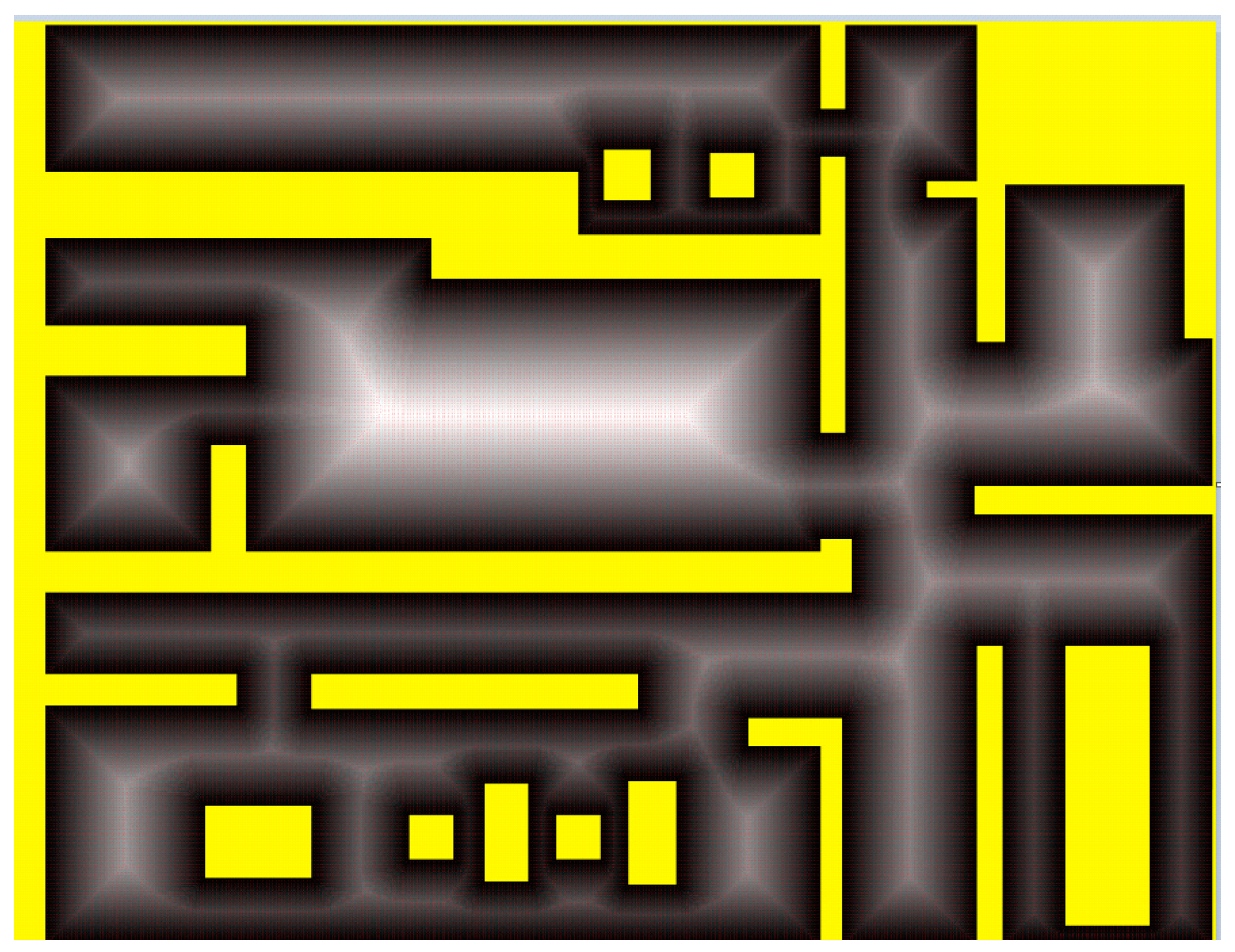
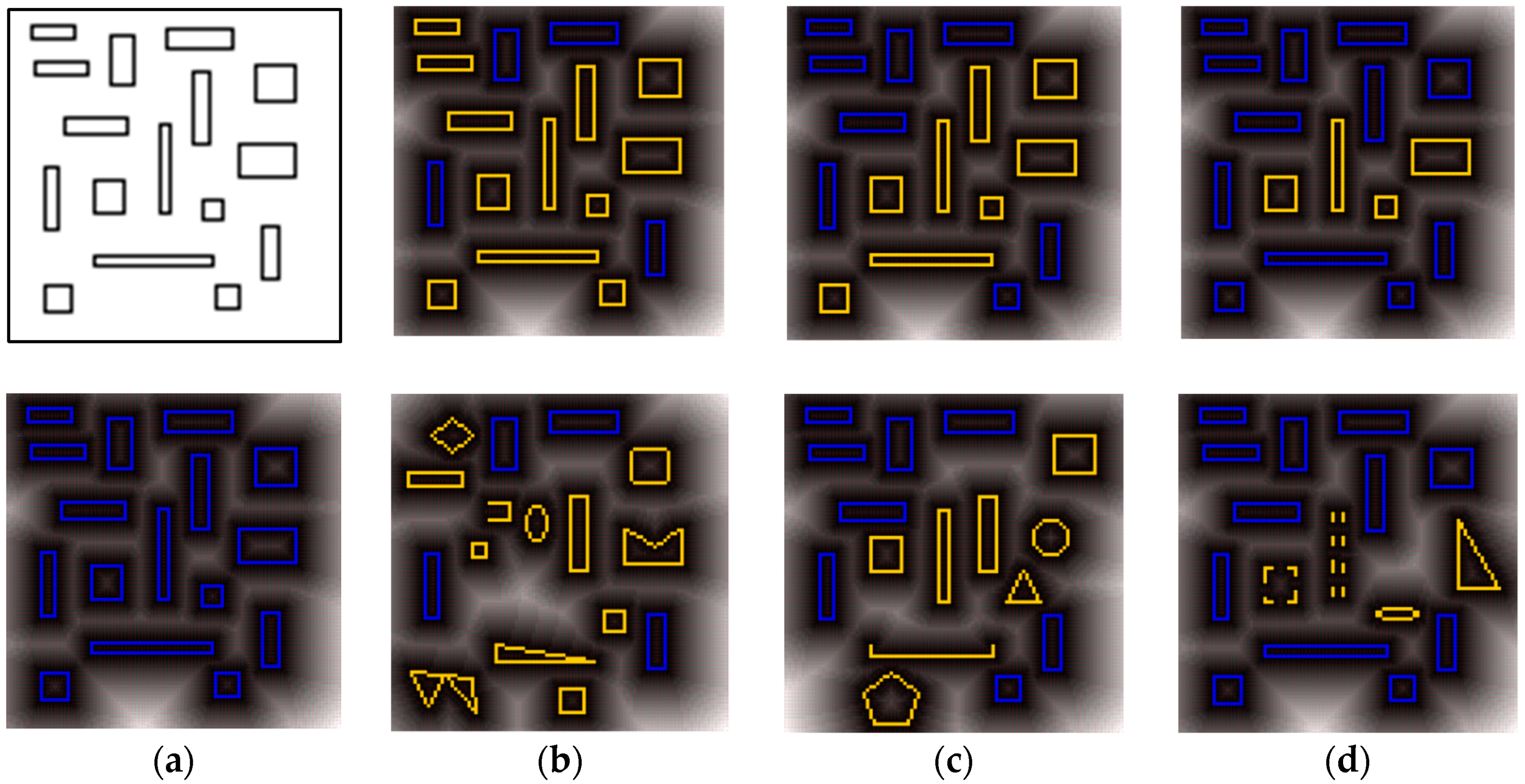
In the context of collision check and path planning in robotics and game AI, the Distance Map (DM) has been widely used as a consistent model to encode the search space [1,2,3,4,5]. In a grid-based environment with regions of blocked cells, a corresponding DM can be constructed to provide each cell a maximal clearance value, which registers the distance from itself to the nearest obstacle. Thus, a DM can help an agent (e.g., a Non-Player Character (NPC) in the video game or a robot in the real world) with a certain safety radius to efficiently search out collision-free paths and to avoid obstacles in motion. Figure 1 presents a DM constructed in an indoor environment.

In many practical applications, the underlying environments that an agent maneuvers in are often dynamic; therefore, it is necessary to reconstruct their corresponding DMs whenever changes of cell states are observed (e.g., an obstacle is inserted, removed, reshaped, or transferred). Since such changes usually occur within a relatively neighboring area around the agent, only portions of the previously constructed DM need repair. To make use of this localized feature, existing algorithms such as Dynamic Brushfire [6] and its subsequent variants [7,8] aim to speed up the reconstruction by launching a wavefront from the source of the state changes to incrementally repair the distance values, rather than reconstructing the whole DM from scratch. With such a localized mechanism, only those cells that are actually affected by the wavefront need to be handled; thus, in most cases, the computation costs can be efficiently reduced.

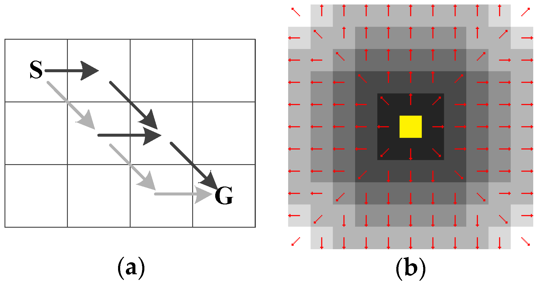
However, for all of the previously proposed algorithms, the propagation of the wavefronts simply expands all the neighbors of a processed cell without preference, and then inserts the newly affected neighbors into a priority queue, so as to prepare for the next round propagation. Such indiscriminate expansion results in a much longer priority queue and thus becomes an efficiency bottleneck. In order to reduce the number of elements which need to be sorted by the priority queue, a searching strategy, Canonical Ordering, is introduced by us to systematically choose a single route from the equivalent propagation paths. 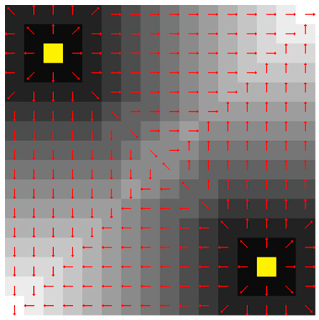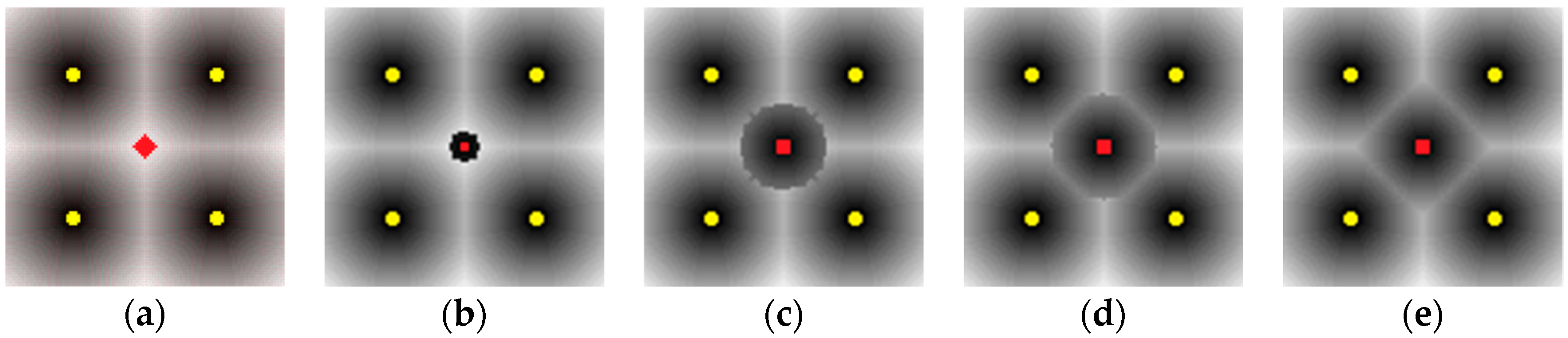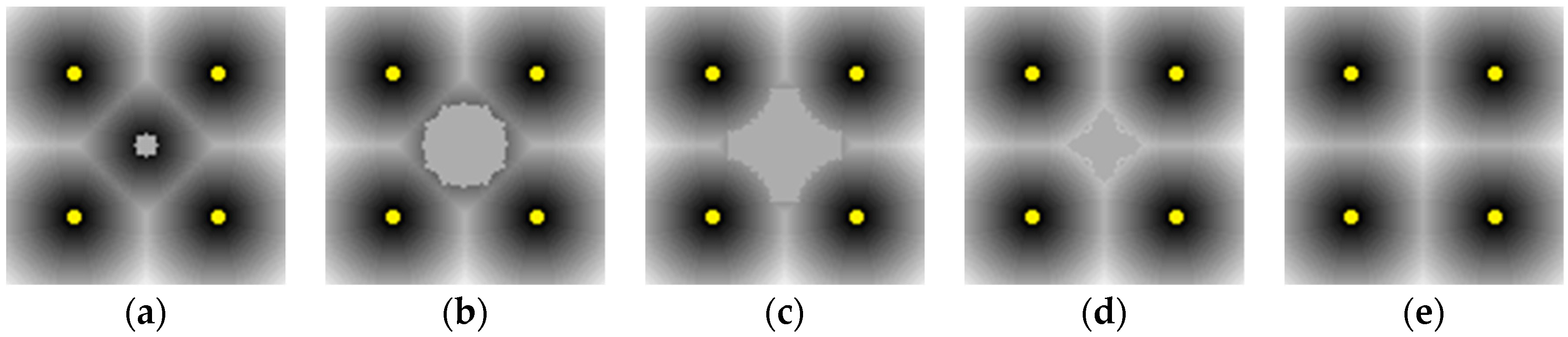Figure 2 shows how our algorithm propagates the wavefront form the source blocked cell (denoted as yellow tiles), visiting each affected cell only once (where the red arrows denotes the propagation directions of the wavefronts). We choose the successors of an expanded cell, s, by following two basic rules described in Nathan R. Sturtevant and Steve Rabin’s paper [9]. That is, for a cell s, with the propagation direction c that was previously used to reach s, (1) If c to arrive at s is one of the four cardinal directions, the only legal direction at s for the next round propagation is c; (2) If the c to arrive at s is one of the four diagonal directions which can be decomposed into two perpendicular cardinal components c₁ and c₂, the legal directions at s for the next round propagation are c, c₁, and c₂. We name our algorithm Canonical Ordering Dynamic Brushfire (abbreviated to CODB in the rest of this paper).

Since a DM stores the maximal clearance for each traversable cell to its nearest obstacle, operations such as collision checks can be simplified to instant look-up queries (As shown in Equation (1)). For instance, if an agent with safety radius R> 0 is located on cell s, then the result of the collision check is determined by Equation (1) as below (where 1 denotes collision detected and 0 denotes collision-free):

$$C\left(R,s\right)=\{\begin{array}{c}1\\ 0\end{array}\begin{array}{c}if\left(R-DM\left(s\right)\right)\ge 0\\ if\left(R-DM\left(s\right)\right)<0\end{array}$$

(1)

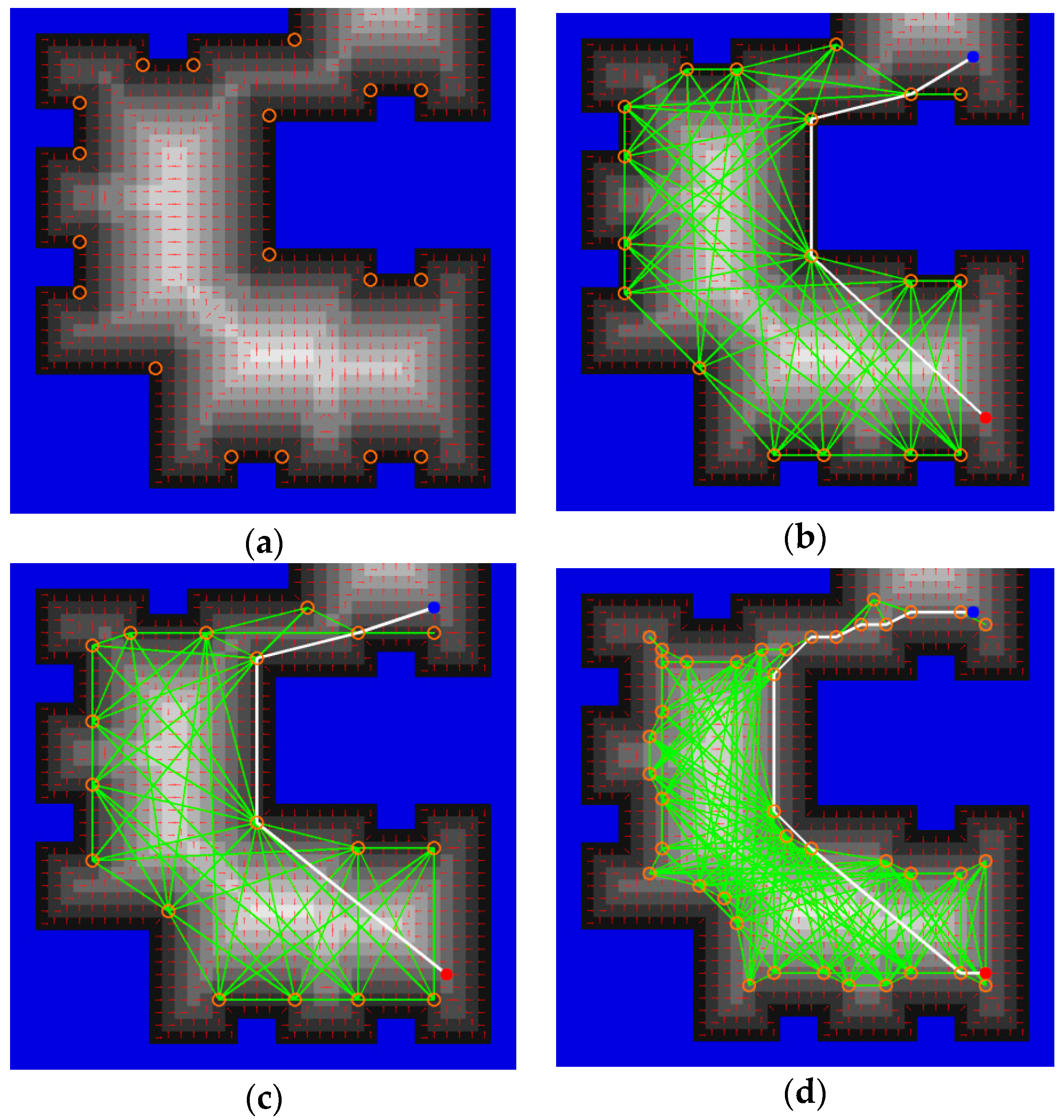
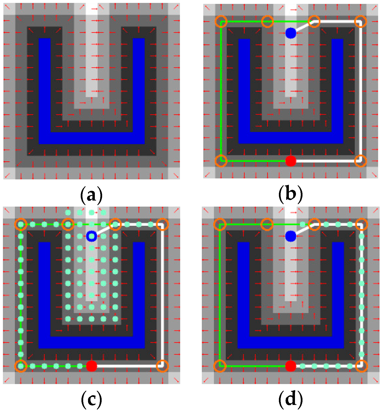
To make better use of this feature, we furthermore propose algorithms to construct DM-based subgoal graphs. The resulting subgoal graphs are sparse but adequate high-level roadmaps to enable agents who possess safety radius to search out collision-free paths in real time. In order to reduce the possibility of replanning caused by dynamic terrain changes, we introduce Learning Real Time A* (LRTA*) [10], an algorithm for planning immediate moves at runtime, to drive the agents between subgoals connected by the high-level paths. Since each segment of the high-level paths is proved to be direct h-reachable, irrational behaviors such as trapping in local minima can be eliminated when LRTA* is iteratively applied between the direct-h-reachable subgoals (see the definition of direct h-reachable in Section 4.1.3).

There is another space representation; i.e., grid-based Voronoi diagrams can be used as a sparse model to help agents to maximize its distance to the obstacle cells. Actually, current algorithms for building grid-based Voronoi graphs can also obtain a corresponding distance map in which each cells keeps the distance to its nearest obstacle cell [11,12,13]. Although a Voronoi diagram can provide an agent with a sparser search space, its drawback is also prominent. For instance, in Multi-Agent Pathfinding Problems (MAPF) [14,15,16,17,18,19], a group of coordinated agents share the same Voronoi edges as their search space, thus a dense cluster of conflicts may occur, which needs to resolve during the planning process. Different from grid-based Voronoi Diagram, DM-based subgoal graphs don’t conservatively compress the search space in unnecessary narrow channels. Furthermore, the search space between each pair of the direct-h-reachable subgoals commonly reserve more spaces than Voronoi edges for a group of coordinated agents to resolve conflicts.

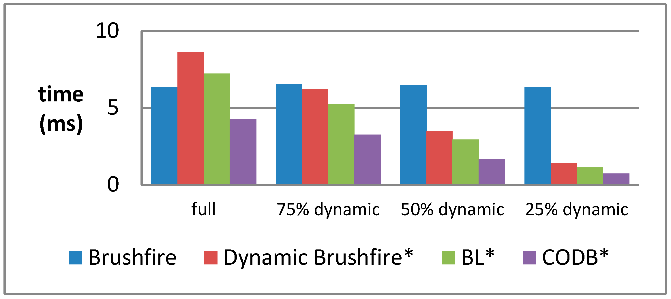
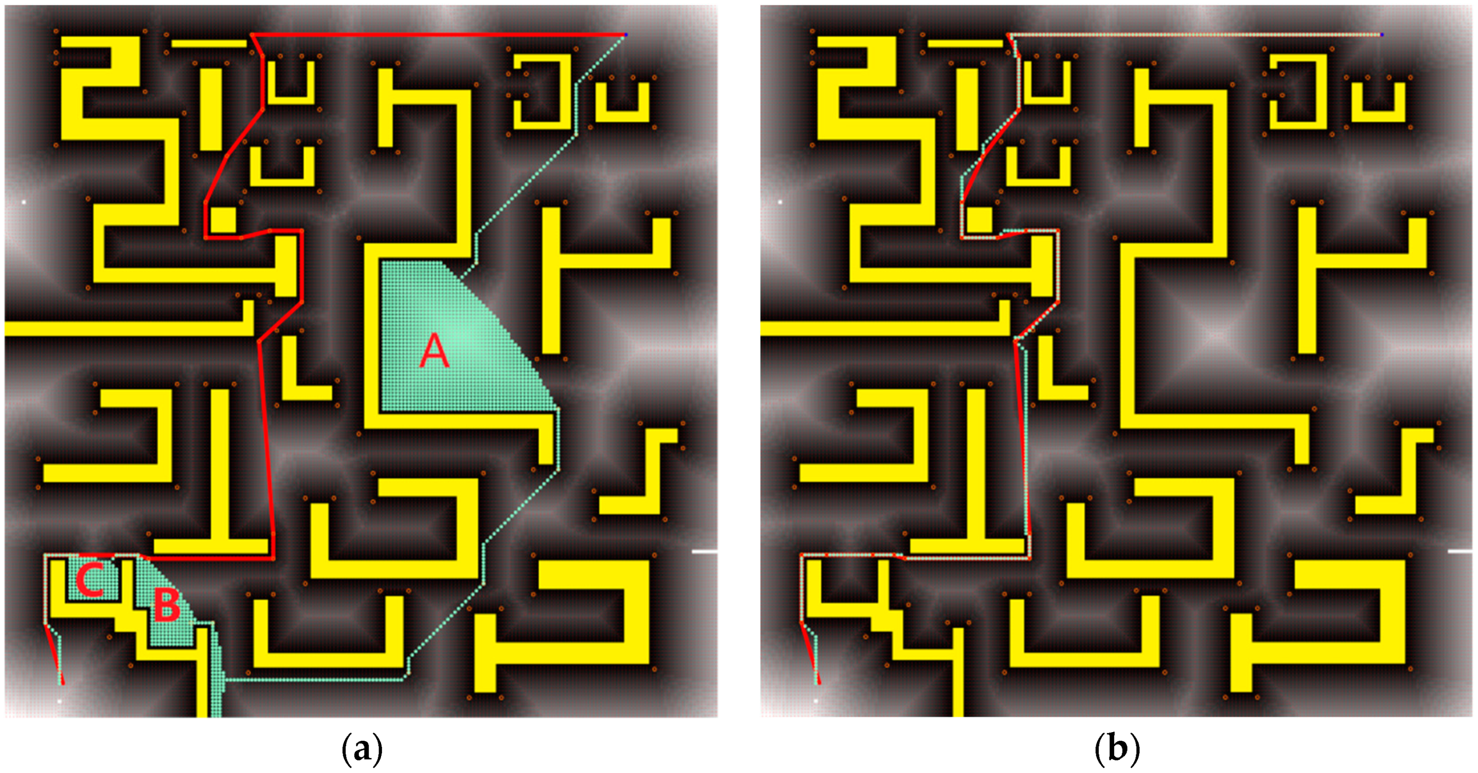
We provide three main contributions in this paper. Firstly, we present an algorithm, Canonical Ordering Dynamic Brushfire (CODB), to speed up the incremental update of grid-based Distance Maps (DMs). Secondly, we propose algorithms to compute DM-based subgoal graphs which are used to provide high-level, collision-free roadmaps for agents with certain safety radius. Thirdly, we verify that under the guidance of the subgoal graphs, real-time search algorithms such as LRTA* can effectively avoid local minima; therefore, the resulting trajectories can successfully coincide with the optimal solutions searched by A*. We present our algorithms both intuitively and through pseudocode, compare them to current approaches on typical scenarios, and demonstrate their usefulness for fast path planning tasks.

The outline of this paper is as follow: Section 2 discusses related studies on DMs, Canonical Ordering, and subgoal graphs; Section 3 gives preliminaries and notations; Section 4 presents our algorithms both intuitively and through pseudocode; Section 5 compares CODB to other algorithms and tests the usefulness of DM-based subgoal graph for fast path planning tasks. This paper ends with conclusions in Section 6.

2. Related Work

2.1. Grid-Based Distance Maps

In the context of robotics and game AI, the grid-based DM is a popular spatial representation applied in navigation and motion planning tasks. The principal component of the recent approaches for constructing or reconstructing grid-based DMs is the well-known Brushfire algorithm [20]. Intuitively, Brushfire launches wavefronts to propagate changes of maximal clearance (i.e., changes caused by insertion or deletion of obstacle cells), updating distance values from the source of the change, and terminates when the change does not affect any more cells. Brushfire represents the OPEN list as a priority queue to incrementally record the affected cells and propagate the wavefronts. The priority of an element in the OPEN queue is determined by its newly updated distance and all these elements are popped up in increasing priorities. Sequentially, new cells which are adjacent to the popped one are tested, among which, newly updated cells will again be inserted into the OPEN list so that the propagation continues.

Kalra et al. [6], in their fundamental work, proposed a dynamic version of Brushfire algorithm, Dynamic Brushfire, to incrementally update grid-based DMs by propagating two kinds of wavefronts named “lower” and “raise” which start at newly blocked or freed cells, respectively; therefore, the update can be constrained within local areas. However, the wavefronts launched by Dynamic Brushfire roughly accumulate 8-connected grid steps to approximate maximal clearance, which overestimates the true Euclidean distances and would possibly lead to either a collision risk or overly conservative movements. To this end, Scherer et al. [21] proposed a method to propagate obstacle locations rather than counts of the grid steps, which reduces the absolute overestimation error below an upper bound of 0.09 pixel units. In the method proposed by Cuisenaire and Macq [22], the shortest distance at which this propagation error can occur is 13 pixels, which yields a maximum relative error of 0.69%. Regarding propagating obstacle references, Lau et al. proposed an approach to provide the location of the closest obstacle rather than just the distance to it, which can be appealing for collision check tasks [23]. Moreover, Lau et al. extended their method to 3D by adding the possibility to limit the propagated distances to maintain online feasibility in large open spaces and outdoors as proposed by Scherer et al.

Although these dynamic algorithms are fast and efficient for dealing with local changes, they just indiscriminately expand all the adjacent cells surrounding a currently processed cell, which results in a lot of redundant cell visits and scales up the size of the OPEN list and restricts the overall efficiency of the algorithm. We introduce the Canonical Ordering strategy in our work to prune the search space.

2.2. Canonical Ordering

The idea of applying Canonical Ordering as a speedup technique for real-time pathfinding systems that operate on regular grids was proposed by Daniel Harabor [24] and N Pochter [25]. As mentioned in the literature, searching in grids often becomes overwhelmed by a high degree of path symmetry, which accounts for a major part of the computational costs. Two paths are viewed as symmetric if (1) they have the same start and goal cells; (2) they are of the same length; and (3) their respective sequences of moves (i.e., cardinal or diagonal moves) can be reordered into the other. With symmetries in the grids, a search task will explore multiple cells for multiple times from those symmetric paths and this severely undermines the efficiency.

To break such symmetries, an online algorithm called Jump Point Search (JPS) [26] was presented by Daniel Harabor et al. to apply Canonical Ordering to recursively prune redundant successors and selectively expand only certain cells, called jump points. Canonical Ordering is essentially a special case of partial orderings among all the symmetric paths and prefers the diagonal-first ones to other alternatives. We say that a path has the diagonal-first property if there is no straight-diagonal turning point can be mutated into a diagonal-straight one of the same length constrained by the obstacles. By its virtue, JPS visits much fewer cells than traditional searching strategies; therefore, it answers a path query averagely faster than A* by an order of magnitude. After that, this algorithm’s performance was further improved by a preprocessing based strategy and addition of Bounding Boxes, resulting in the algorithms JPS+ [26] and JPS+BB [27]. As an automatic move pruning technique for single-agent search [28], Canonical Ordering can not only be used in grids, but can also be built on general graphs and considerably reduce the number of cells generated by an A* search [29].

The outstanding performance of the Canonical Ordering strategy in compressing search space for real-time pathfinding algorithms provides us with a novel method to guide the direction of the wavefronts which propagate the distance changes, making it possible to speed up the construction of grid-based DMs.

2.3. Subgoal Graphs

A subgoal graph is a kind of sparse spatial representation which can be precomputed by abstracting the skeletons of the underlying grids into undirected graphs. The algorithm which accounts for computing subgoal graphs was proposed by Tansel Uras et al. [30]. It firstly introduces the basic version of the subgoal graph, called Simple Subgoal Graphs (SSGs). On grid maps, SSGs are constructed by placing subgoals at the convex corners of obstacles and connecting direct-h-reachable subgoals in the preprocessing stage. Two subgoals are mutually direct-h-reachable if all the optimal paths between them are valid and traverse no other subgoals.

SSGs reduce the search space and accelerate the process of finding shortest paths by abstracting the key points of the grid maps and reducing all symmetric paths between subgoals into only one edge. It can be proved that, for any given start and goal cells which are reachable, there is a shortest path that can be divided into segments between subgoals. Each segment connects direct-h-reachable subgoals. Therefore, when finding shortest paths on SSGs, one first connects the start and goal vertices to their direct-h-reachable subgoals in SSGs, and then searches the modified graphs via A* to get the shortest high-level path, which consists of a sequence of subgoals between the start and goal vertices. By refining the shortest high-level path, one can get the shortest path between start and goal on the grid map.

Moreover, a Two-level Subgoal Graph (TSG) is constructed from a SSG by partitioning the subgoals into global and local ones and only the global ones belong to the TSG. When removing the local subgoals, one has to add some extra edges so that the shortest paths between global subgoals remain the same. Finding the shortest path on a TSG is similar to finding a shortest path on a SSG. One first connects the start and goal vertices to their direct-h-reachable subgoals, among which the local ones should be temporarily connected to the TSG. Then, the search and refining processes are executed. It should be noted that the refining process of TSGs is slower than SSGs because TSGs connect h-reachable subgoals instead of direct-h-reachable subgoals. But, TSGs still find optimal paths faster due to the smaller search space. To reduce the search space even further, Tansel Uras et al. generalized the idea of partitioning [31,32], created a hierarchy among the vertices, and repeatedly divided the highest-level subgoals into global and local subgoals and increased the level of global subgoals by one. The resulting graphs are called N-Level Subgoal Graphs.

Subgoal Graphs can be used not only to find grid paths, but also to find any-angle paths which are shorter and more realistic [33,34,35]. Tansel Uras and Sven Koenig [36] exploited the similarities between Subgoal Graphs and visibility graphs and used Subgoal Graphs to quickly find any-angle paths with some small modifications. Their algorithm is up to two orders of magnitude faster than Theta*, a well-known any-angle path planning algorithm.

All the above algorithms only take regular grids as input and build subgoal graphs which do not take physical radius into considerations. Therefore, the paths planned from the resulting subgoal graphs would possibly be unable to meet the collision-free requirements in practical application. In this paper, we attempt to modify the existing algorithm so that it can make use of the maximal clearance values provided by the grid-based DMs and to build new type of subgoal graph that can efficiently search collision-free paths.

3. Preliminaries and Notation

All the algorithms studied in this paper work in planar, eight-connected grid maps with regions of obstacles consisting of blocked cells. A wavefront launched by a cell state change can propagate from one cell to its neighbor in any cardinal or diagonal directions, and the length of the cardinal and diagonal moves are 1 and $\sqrt{2}$, respectively. We follow the definition of octile distance to compute the heuristic distance between any two cells in a grid map, i.e., the distance between cells s and s’ is computed by following Equation (2):

$$dist\left(s,s^{\prime }\right)=\sqrt{2}\times min\left(dx,dy\right)+\left|dx-dy\right|$$

(2)

In Equation (2), dx and dy denote the differences of the 2D coordinates of cell s and s’. For each cell s, obst_s maintains coordinates of the obstacle cell s_o to which s is currently closest, and dist_s maintains the distance between s and s_o. The notation dir_s maintains the direction along with which s would propagate the wavefront. The options of dir_s include four cardinal directions (denoted as left = 1, up = 3, right = 5, and down = 7), four diagonal directions (denoted as up-left = 2, up-right = 4, down-right = 6, and down-left = 8), and full directions (denoted as full-dir = 0, declaring that s is the source of the wavefront; thus, all the eight directions need to be considered in the next round propagation). The notation raise_s shows if the wavefront on s is a raise wavefront or a lower one (the differences between raise and lower wavefronts are explained in Section 4.1.1). Given a cell s, a direction d, and an integer k, the notation s’ = s + kd denotes a cell s’ that is reached from s by moving k steps along d. For two perpendicular directions c₁ and c₂, we have d=c₁+c₂ to denote that the sum of c₁ and c₂ results in their corresponding diagonal direction d.

4. The Methodology

4.1. Algorithm Intuition

Figure 3 shows the flowchart describing the main steps of CODB and its application in real-time pathfinding tasks.

4.1.1. Lower and Raise Wavefronts

Following the basic ideas of Dynamic Brushfire algorithms, CODB employs two kinds of wavefront, lower and raise wavefronts, to incrementally update DMs. CODB keeps a priority queue (denoted as OPEN) to sort the cells to be explored by the wavefronts. A cell’s priority is determined by its dist_s value and is dequeued with increasing priority values. When a cell is popped from OPEN, the distance change on it will be propagated to its adjacent cells and any inconsistent cells (i.e., cells which are affected by the wavefront) are again put on OPEN, so as to prepare for the next round of propagation.

As shown in Figure 4a, when an obstacle cell (red dot denoted as s) is newly inserted into the center of the grids, it firstly sets dist_s as 0 and obst_s as its own coordinates; then, a so called “lower wavefront” is launched to propagate a distance reduction to its adjacent cells (as shown in Figure 4b). This propagation emanates from s, the source of the change, and terminates when the distance change no longer affects anymore cells (as shown in Figure 4c,d, the wavefront encounters cells which keeps equal clearance to other obstacle cells and thus failed to continue the propagation.). Finally, new boundaries of the updated DM are reached and the distance values of all affected cells are updated (As shown in Figure 4e).

On the other hand, when an obstacle cell is removed (e.g., as Figure 5a shows, we again remove the center obstacle cell s from the map), all the cells whose obst and dist value are computed based on s become invalid; therefore, a so called “raise wavefront” is launched to reset these invalid cells, declaring that they can be then updated by other lower wavefronts (as shown in Figure 5b). The “raise wavefront” terminates at the boundaries between s and other obstacle cells (as shown in Figure 5c), then lower wavefronts on the other sides of the boundaries are permitted to continue their propagation until the invalid region is again submerged (as shown in Figure 5d) and Figure 5e).

4.1.2. Propagation in Canonical Ordering

To speed up the construction efficiency, we introduce the concept of Canonical Ordering to guide the propagation of wavefronts. The application of Canonical Ordering has been recently discussed to speed up best-first search in grids-based pathfinding tasks in [24]. Different from the classical Dynamic Brushfire algorithm, which expands all the eight directions at every step, Canonical Ordering can eliminate redundant, symmetric paths from the source of state change, which accounts for the main part of the speed improvement.

As shown in Figure 6a, in an open grid map without obstacles, a wavefront launched by a cell (denoted as s) on the left top can follow three different optimal paths to propagate its distance change to the traversable cell (denoted as g) on the right bottom. The only difference between these paths relies on the permutation of actions of moving right one cell and moving down-right two cells. It is clear to see that the number of possible paths grows exponentially if we enlarge the grid map and keep g in the right bottom corner. Since the existing Dynamic Brushfire algorithm generates the same cell along different paths, such propagation would trigger large numbers of pushing and sort ascending operations in OPEN list, which can be computationally expensive.

To eliminate these redundancies, Canonical Ordering insists on a preference rule, i.e., distance changes first propagate diagonally before propagating cardinally whenever possible along a path (e.g., as shown in Figure 6a, by following this rule, only the gray path is tested.). With such a preference, a source cell in an open grid map returns a unique path from itself to each affected cell. As shown in Figure 6b a wavefront launched from the center cell (denoted as a yellow cell) draws lines diagonally and then branches vertically and horizontally, extending from the diagonals. Since every affected cell owns exactly one path from the source cell, the propagation is no longer a graph, but a tree.

4.1.3. DM-Based Subgoal Graph

In order to introduce the concept of maximal clearance provided by DMs into the precomputing algorithms of subgoal graphs, we extend the formal definitions of the traditional subgoal graph as follows:

Definition 1. 

For two cells s and s’, let dx and dy be the respective distances between s and s’ along the x and y axes. The shortest trajectory between s and s’ is a permutation of exactly min(dx,dy) diagonal and |dx-dx| cardinal moves, for a total of max(dx,dy) moves.

Definition 2. 

Given a safety radius R, a collision-free path between two cells s and s’ is the shortest trajectory in which each cell s^{^} is collision-free, i.e., C(R,s^{^})=0.

Definition 3. 

Given a safety radius R, an unblocked cell s is a collision-free subgoal if there are two perpendicular cardinal directions c₁ and c₂ such that C(R,s+c₁+c₂)=1, C(R,s+c₁)=0 and C(R,s+c₂)=0.

Definition 4. 

Given a safety radius R, two cells s and s’ are h-reachable if there is a collision-free path of octile length h(s,s’) between them. Two h-reachable cells are safe-h-reachable if all shortest trajectories between them are also paths. Two safe-h-reachable cell s and s’ are direct-h-reachable if none of the shortest paths between them contains a subgoal s’’ $\notin$ {s,s’}.

Definition 5. 

Given a safety radius R, an DM-based subgoal graph, Gs =(R,Vs,Es), on its corresponded grids, is a high-level, undirected graph, where Vs is the set of collision-free subgoals and Es is the set of edges connecting direct-h-reachable subgoals, and the length of the edges is the octile distances between the subgoals they connect.

The process of constructing an DM-based subgoal graph can be intuitively divided into two steps: (1) placing collision-free subgoals at the corners of the expanded obstacle boundary to circumnavigate the collision regions (e.g., the orange circles shown in Figure 7a); (2) adding edges between those subgoals which are mutually direct-h-reachable (e.g., the green edges shown in Figure 7b). Given a start and a goal cell (e.g., the blue and red discs shown in Figure 7b), we first connect them to their respective direct-h-reachable subgoals and then plan a high-level shortest path by executing A* on the updated subgoal graph (e.g., the white trajectory shown in Figure 7b). We can refine each segment of the high-level path by arbitrarily selecting an h-reachable path between two connecting subgoals, and then orderly appending these refined paths together. Moreover, as shown in Figure 7c,d, for agents with different safety radius, their corresponding DM-based subgoal graph, according to Definition 5, can set aside adequate clearance; therefore, the paths found from the resulting graphs can be collision-free.

4.2. Algorithm Pseudocode

4.2.1. Initiate the DM

Table 1. The pseudocode for initialization.

initialize() 1. OPEN$\leftarrow$$\varnothing$ 2. for each cell s in the grid map do 3.  dists $\leftarrow$ $\infty$ 4.  obsts $\leftarrow$ $\varnothing$ 5.  voros $\leftarrow$ false 6.  raises $\leftarrow$ false 7.  dirs $\leftarrow$ 0

setObstacleCell (Cell o) 8.  disto $\leftarrow$ 0 9.  obsto $\leftarrow$ o 10. insert (OPEN,o,0)

removeObstacleCell (Cell o) 11. resetCell (o) 12. raiseo$\leftarrow$true 13. insert (OPEN, o, 0)

presents pseudocode for the initialization of a DM, including three functions, i.e., (1) initialize() to set aside certain space for required data structures and then initial their values; (2) setObstacleCell(o) to register a newly inserted obstacle cell; and (3) removeObstacleCell(o) to reset an removed obstacle cell. Upon initialization, all the cells are set to be traversable and undetermined, declaring that there is no obstacle cell, neither in the map, nor in finite distance (lines 1 to 7). When a cell o is marked as an obstacle cell by calling setObstacleCell(o), it sets dist_o as 0 and refers to itself as the closest obstacle cell, i.e., obst_o = o (lines 8 and 9). Conversely, when o is freed by calling removeObstacleCell(o), the function resetCell(o) resets it to the initial values, i.e., dist_o = $\infty$ and obst_o = ∅ (line 11), and raise_o is set as true (line 12). The function insert (OPEN, c, d) inserts a cell c into OPEN with a priority value d, or updates the priority if c is already in OPEN.

4.2.2. Update the DM

Table 2. The pseudocode for updating the Euclidean distance map.

update() 14. whileOPEN$\ne \varnothing$do 15  s $\leftarrow$ pop(OPEN) 16.  if raises then 17.   raise(s) 18.  else if isOcc(obsts) then 19.   voros $\leftarrow$ false 20.   lower(s)	lower (cell s) 21. N$\leftarrow$ findSuccessors(s) 22. for eachn$\in$Ndo 23.  if $\neg$raisen then 24.   d $\leftarrow$ distance (obsts,n) 25.   if d $<$ distn; then 26.    distn $\leftarrow$ d 27.    obstn $\leftarrow$ obsts 28.    dirn $\leftarrow$ direction(s,n) 29.    insert(OPEN,n,d)	raise (cell o) 30. N$\leftarrow$ findSuccessors(s) 31. for eachn$\in$Ndo 32.  if (obstn $\ne \varnothing \bigwedge \neg$raisen) then 33.   if $\neg$ isOcc(obstn) then 34.    clearCell(n) 35.    raisen $\leftarrow$ true 36.    dirn $\leftarrow$ direction(s,n) 37.   else dirn $\leftarrow$ full-dir 38.   insert (OPEN,n,distn) 39. raises$\leftarrow$false
findSuccessors(cell s) 40. ifdirs is one of the four cardinal directions then 41.   return N $\leftarrow$ {s + dirs } 42. else 43.   return N $\leftarrow$ {s + dirs, s + c1, s+c2 | where dirs =c1+c2}

presents pseudocode for updating the DM. The function update() orderly pops the next unprocessed cell s with the lowest dist_s until the OPEN queue is empty (lines 14 and 15). If s is cleared and is not yet propagated by a raise wavefront, the function raise() is called (lines 16 and 17). However, if s has a valid closest obstacle cell, the function lower() is called (lines 18 to 20).

Newly inserted obstacle cells call function lower() to launch a lower wavefront to propagate the reduction of dist and obst values from the currently popped cell s to its affected cells (lines 26 to 29). The lower wavefront continues when the distance value (denoted as d which is computed in line 24) between obst_s and the newly expanded cell n holds the trend of distance reduction (being determined in line 25). Simultaneously, newly freed cells call function raise() to launch a raise wavefront, resetting the cells whose closest obstacle cell was the freed one (line 33 to 36). The raise wavefront terminates when it reaches those cells whose closest obstacle is valid; thus, a lower wavefront launched by n is generated (line 37). During the interwoven of these two wavefronts, inconsistent neighbors affected by the processed cell are again put on OPEN (line 29 and 38), thus the propagation continues.

Instead of propagating a wavefront along with full directions, we introduce a function findSuccessors(s) to filter cells by employing the rule of canonical ordering (line 21 and 30). As illustrated in Figure 6b, only the successors of a cell in the direction of the arrows are chosen as the candidates of the next round of propagation, while the others are ignored. For a cell n conducting a wavefront from one of its adjacent cell s, function direction(s,n) determines the direction from s to n and accordingly returns the value of dir_n (line 28 and 36).

4.2.3. Construct DM-Based Subgoal Graphs

By making use of the collision test equation shown in Equation (1), we modify the subgoal placement condition of the original construction algorithm; therefore. a collision-free subgoal graph for a certain safety radius R can be efficiently computed from the underlying DM.

Given an agent with safety radius R $\ge$ 0,

Table 3. The pseudocode for constructing DM-based subgoal graphs.

ConstrucDMBasedSubGraph(safetyRadius R) 44. Vs$\leftarrow \varnothing$, Es$\leftarrow \varnothing$ 45. for eachunblocked cells sdo 46.  for each pair of perpendicular cardinal directions c1 and c2 do 47.   if C(R,s+c1+c2)=1 then 48.     if C(R,s+c1)=0$\wedge$C(R,s+c2)=0 then 49.      Vs $\leftarrow$ Vs${{\displaystyle \bigcup }}^{}${s} 50. for each s $\in$ Vs do 51.  S$\leftarrow$ GetDirectHReachable(Vs, R,s) 52.  for each s’$\in$S do 53.   Es $\leftarrow$ Es${{\displaystyle \bigcup }}^{}${(s,s’)} 54. Gs$\leftarrow$ (Vs,Es)

shows how to construct a subgoal graph, Gs := (Vs,Es), from the underlying DM. The entire construction process consists of two sequential phases, i.e., firstly placing collision-free subgoals on the corners of the expanded obstacle boundaries (line 45 to line 49), and secondly, adding edges to connect those subgoals which are mutually direct-h-reachable (line 50 to 53).

A time-consuming and important part in the algorithm shown in Table 3 is how to identify all direct-h-reachable subgoals from a given subgoal s (line 51), and this can be done by determining the direct-h-reachable area around s. As shown in

Table 4. The pseudocode of determining the direct-h-reachable area of a given unblocked cell s.

GetDirectHReachable(subgoals V, safetyRadius R, cell s 55. S$\leftarrow \varnothing$ 56. for eachdirections ddo 57.  s’ $\leftarrow ($s+SafeClearance(R,V,s,d)$\times$d$)$ 58.    if s’ $\in$ V then S $\leftarrow$ S${{\displaystyle \bigcup }}^{}${s’} 59. for eachdiagonal directions ddo 60.  for each cardinal directions c associated with d do 61.   max $\leftarrow$ SafeClearance(R,V,s,c) 62.   diag $\leftarrow$ SafeClearance(R,V,s,d) 63.   if ((s+max)$\times$c) $\in$ V) then max $\leftarrow$ max-1 64.   if ((s+diag)$\times$d) $\in$ V) then diag $\leftarrow$ diag -1 65.   for each i from 1 to diag do 66.    j $\leftarrow$ SafeClearance(R,V,s+id,c) 67.   if j$\le$max and $($s+id+c) $\in$ V then 68.     S $\leftarrow$ S${{\displaystyle \bigcup }}^{}$ {s+id+c} 69.     j $\leftarrow$ j-1 70.    if j<max then max $\leftarrow$ j

SafeClearance(safetyRadius R, subgoals V, cell s, direction d) 71. i$\leftarrow$0 72. whiletruedo 73.  if $\neg$(C(R,s+id) = 0$\wedge$ C(R,s+id+d)=0) then 74.   return i 75.  i $\leftarrow$ i+1 76.  if (s+id) $\in$ V then return i

the algorithm proposed by Tansel Uras et al. [30] works in two steps. The first step (line 56 to 58) identifies the closest subgoals in each of the eight cardinal and diagonal directions, and the second step (line 59 to 70) incrementally finds out the other subgoals that can be reached via moves in two directions (i.e., either a diagonal direction or one of its two corresponded cardinal directions). In order to meet the strong requirements of Definition 5, we replace the Clearance(R, V, s, d) function in the original algorithm with SafeClearance(R, V, s, d), thus the resulting direct-h-reachable paths between two subgoals can be collision-free when taking safety radius R into consideration (e.g., the tests in line 73 ensure that every step of the incremental exploration is collision-free). For more detail about the function GetDirectHReachable, please refer to Tansel Uras’ work [30].

4.2.4. Find Paths in DM-Based Subgoal Graphs

The algorithms shown in

Table 5. The pseudocode for searching paths in DM-based subgoal graphs.

FindHighLevelPath(subgoals V, edges E, safetyRadius R, startCell s, endCell s’) 77. ConnectToGraph(V,E,R,s) 78. ConnectToGraph(V,E,R,s’) 79. Π$\leftarrow$ A*(V,E,s,s’) 80. restore original graph 81 return Π

ConnectToGraph(subgoals V, edges E, safetyRadius R, cells s) 82. ifs$\in$Vthenreturn 83.  Vs $\leftarrow$ Vs${{\displaystyle \bigcup }}^{}${s} 84.  S $\leftarrow$ GetDirectHReachable(V,R,s) 85.  for each s’$\in$S do Es $\leftarrow$ Es${{\displaystyle \bigcup }}^{}${(s,s’)}

are proposed by Tansel Uras et al. [30], illustrating how to search for a high-level path between two cells in the subgoal graphs. The function FindHighLevelPath is called to connect s and s’ to the underlying subgoal graph, engage an A* search to find a shortest collision-free path between s and s’ from the updated subgoal graph (line 79), and to restore the original graph (line 80) before returning the resulting path (line 81). The function ConnectToGraph is called to identify all direct-h-reachable subgoals of s and s’ (line 77 and line 78), and then add new edges between them into the graph (line 85)).

According to Tansel Uras’ work, the real-time requirement is easy to meet because each segment of the resulting high-level path can be quickly refined by arbitrarily choosing one of the symmetric paths between its two direct h-reachable subgoals. However, this global planning strategy often fails in some dynamic environments in which some other moving agents may block the preplanned routes. To solve this problem, we introduce Learning Real-time A* (LRTA*), a real-time heuristic search algorithm [10], to take local changes into consideration and repeatedly plan and execute actions within a constant time interval during the runtime.

We illustrate the key idea of LRTA* via pseudocode shown in

Table 6. The pseudocode for learning real time A* search.

LRTA*(start s, end s’, safety radius R) 86. s^$\leftarrow$s 87. while s^$\ne$s’ do 88.  S $\leftarrow$ frontier(s^,R) 89.  s’’ $\leftarrow argmi{n}_{n\in S}$ (g(s,n)+h(n,s’)) 90.  h(s^,s’) $\leftarrow$ g(s,s’’)+h(s’’,s’) 91.  s^ $\leftarrow$ s’’

. As long as the goal cell s’ is not reached (line 87), the agent will follow the plan (line 88 and 89), learn (line 90), and execute the (91) cycle. The planning phase expands all the traversable, reachable cells within the range of a fixed look ahead range R and choose one cell n with the lowest g(s,n)+h(n,s’) as the immediate goal for the next move (line 89). During the learning part, the numeric value h(s^,s’) is updated to approach the real total cost, denoted by h*(s^,s’) (line 90). Finally, the agent moves by changing its current position towards the most promising cell discovered in the planning phase (line 91).

A drawback that prevents the application of LRTA* is that agents who adopt this strategy could possibly be trapped in local minima [37]. As shown in Figure 8a, local minima often exist around certain terrain patterns such as concave regions, long distance barriers, and so on. Agents who use LRTA* to search paths in these patterns would meaninglessly move back and forth, visit the same cells several times to correct their heuristic values before escaping from these regions (As shown in Figure 8c). However, the high-level path planned from the DM-based subgoal graph can provide an agent with waypoints which circumnavigate the collision regions (As shown in Figure 8b). Therefore, it can efficiently evade local minima by iteratively popping subgoals from the high-level path as the next waypoint to head for (as shown in Figure 8d).

5. Experiments and Results

In this section, we employ statistical methods to compare our algorithm with other competing methods on certain simulated scenarios. We also demonstrate the usefulness of the DM-based subgoal graphs to real-time path planning tasks. Our algorithms are implemented in C++, running on an Intel® Core(TM) i7-4790 CPU @ 3.60GHz.

5.1. Comparison to Other Algorithms

We compare CODB with other three competing algorithms (i.e., Brushfire, Dynamic Brushfire, and algorithms proposed by Boris Lau et al. [23] (we abbreviate it as BL below)) which are discussed in Section 2 in four typical scenarios as shown in Figure 9.

We set aside four grid maps (from Figure 9a to Figure 9d) which have the same size (100 × 100) while allowing different proportions of the obstacles (i.e., fully reconstruction, 75%, 50%, and 25% respectively) to randomly change their positions or shapes. After each set of changes, we use the above mentioned four algorithms to construct or reconstruct the DMs. We run each algorithm on each scenario 100 times, and the comparisons of the performances among these algorithms are shown in

Table 7. Comparison of the algorithms’ efficiencies in the four scenarios (milliseconds).

Algorithm	Full Reconstruction		75% Dynamic		50% Dynamic		25% Dynamic
	μ	$\mathit{\sigma }$	μ	$\mathit{\sigma }$	μ	$\mathit{\sigma }$	μ	$\mathit{\sigma }$
Brushfire	6.34	0.2533	6.53	0.1824	6.48	0.2316	6.32	0.2339
Dynamic Brushfire *	8.61	0.1753	6.19	0.2018	3.48	0.1899	1.39	0.2037
BL *	7.22	0.2451	5.24	0.2342	2.93	0.2171	1.12	0.1746
CODB *	4.26	0.2124	3.25	0.1937	1.67	0.2248	0.73	0.2102

* Dynamic algorithms that only repair the affected portions.

and Figure 10 (i.e., the average computation time scaled in milliseconds and its variance) and

Table 8. Comparison of the maximal size of the priority queue OPEN (Only dynamic algorithms are compared).

Algorithm	Full Reconstruction		75% Dynamic		50% Dynamic		25% Dynamic
	μ	$\mathit{\sigma }$	μ	$\mathit{\sigma }$	μ	$\mathit{\sigma }$	μ	$\mathit{\sigma }$
Dynamic Brushfire	27,550	149	24,899	110	16,765	124	13,184	96
BL	12,523	78	10,268	106	8024	95	5327	77
CODB	9048	90	7611	121	6027	102	4116	88

and Figure 11 (i.e., the maximal size of the priority queue OPEN during construction and its variance).

For the first scenario in which full reconstructions are inevitable since all the obstacles are moved or reshaped, the extra operations that enable local repairs make Dynamic Brushfire (8.61 ms) and BL (7.22 ms) slower than their static counterpart, Brushfire (6.34 ms). However, due to the integration of Canonical Ordering strategy, CODB can substantially prune the search space; thus, it still maintains an obvious advantage over the other three algorithms in time efficiency (4.26 ms), even in the case of full reconstructions. As for the other three scenarios, as the proportion of the dynamic obstacles decreases, dynamic algorithms gradually manifest their superiority in speed. Among the three dynamic algorithms, CODB is also faster than the others due to fewer cell visits, reducing the computation time by at least 50%.

5.2. Application Tests on Real-Time Pathfinding

This work is motivated by the need to engage real-time and collision-free pathfinding tasks for agents with a certain safety radius. Such agents often maneuver in dynamic, crowded environments, and have to decide their next move in a limited amount of time. In order to demonstrate the usefulness of our algorithm in such scenarios, two agents (denoted as agent X and agent Y) working in a grid map of size 200 × 200 (as shown in Figure 12) are simulated. For each round of testing, both of the two agents are assigned the same start and goal cells located on the top right and left bottom of the grid map, respectively. The resulting paths of Agent X and Y are respectively shown in Figure 12a,b as light green trajectories; by contrast, the optimal path searched by the classical path planning algorithm, A*, is marked as red trajectories. Agent X simply adopts LRTA* to directly search and move in the underlying DM, while agent Y shown in Figure 12b would firstly search out a high-level path from the DM-based subgoal graph, and then engages LRTA* to search and move between the segments of the path. In order to gain the average performance, we run the test of each of the ten pairs of start and goal cells 100 times.

For agent X, applying LRTA* to engage a real-time search can help the agent successfully avoid collisions with obstacles, but it is very easy for the underlying DM to generate local minima around typical locations such as concaves, narrow channels, long distance barriers, and so on. To the cells within these locations, the occurrence of the local minima results in an increase in errors between the default heuristic values and the actual values. Therefore, LRTA* has to recheck these cells many times to incrementally correct their heuristic values (as shown in line 90, Table 6). Only in this way can the heuristic depressions be gradually filled up and finally drive the agent to escape from the local minima. Unfortunately, such runtime correction incurs meaningless movements (As the regions labeled as A, B, and C in Figure 12a) which are unacceptable to the requirements of engaging reasonable behavior.

As for agent Y, a high-level path (as the red path shown in both Figure 12a,b, is firstly searched out from the DM-based subgoal graph by executing the algorithms proposed in Table 5 (in order to make the figures clear, we only retain the subgoals and do not draw the direct-h-reachable edges). The resulting path provides a list of sparse and direct-h-reachable waypoints to circumnavigate the collision regions. Based on the path, agent B uses LRTA* at runtime to search and move along the path; therefore, it can efficiently avoid local minima and terminate meaningless movements.

6. Conclusions

In this paper, we present an algorithm, Canonical Ordering Dynamic Brushfire (CODB), to speed up the incremental updating of grid-based Distance Maps (DMs). CODB only updates those cells which are affected by local changes, and it employs the strategy of Canonical Ordering to guide the search direction; therefore, the algorithm requires much fewer cell visits and less computation costs compared to its competing approaches. Furthermore, we propose algorithms to compute DM-based subgoal graphs which are used to provide high-level, collision-free roadmaps for agents with certain safety radius to engage fast and rational path planning tasks. We present our algorithms both intuitively and through pseudocode, compare them to current approaches on typical scenarios, and demonstrate their usefulness for fast path planning tasks.

References

1. Chen, L.; Chuang, H.Y. A Fast Algorithm for Euclidean Distance Maps of a 2-D Binary Image. Inf. Process. Lett. 1994, 51, 25–29. [Google Scholar] [CrossRef]
2. Yazici, A.; Kirlik, G.; Parlaktuna, O.; Sipahioglu, A. A Dynamic Path Planning Approach for Multirobot Sensor-Based Coverage Considering Energy Constraints. IEEE Trans. Cybern. 2017, 44, 305–314. [Google Scholar] [CrossRef] [PubMed]
3. Borgefors, G. Distance Transformations in Digital Images. Comput. Vis. Gr. Image Process. 1988, 34, 344–371. [Google Scholar] [CrossRef]
4. Fabbri, R.; Costa, L.D.F.; Torelli, J.C.; Bruno, O.M. 2D Euclidean Distance Transform Algorithms: A Comparative Survey. ACM Comput. Surv. 2008, 40, 1–44. [Google Scholar] [CrossRef]
5. Charrow, B.; Kahn, G.; Patil, S.; Liu, S.; Goldberg, K.; Abbeel, P.; Michael, N.; Kumar, V. Information-Theoretic Planning with Trajectory Optimization for Dense 3D Mapping. Robot. Sci. Syst. 2015, 11. [Google Scholar]
6. Kalra, N.; Ferguson, D.; Stentz, A. Incremental Reconstruction of Generalized Voronoi Diagrams on Grids. Robot. Auton. Syst. 2009, 57, 123–128. [Google Scholar] [CrossRef]
7. Lau, B.; Sprunk, C.; Burgard, W. Efficient Grid-Based Spatial Representations for Robot Navigation in Dynamic Environments. Robot. Auton. Syst. 2013, 61, 1116–1130. [Google Scholar] [CrossRef]
8. Qin, L.; Yin, Q.; Zha, Y.; Peng, Y. Dynamic Detection of Topological Information from Grid-Based Generalized Voronoi Diagrams. Math. Probl. Eng. 2013, 2013, 1–11. [Google Scholar] [CrossRef]
9. Sturtevant, N.R.; Rabin, S. Canonical Orderings on Grids. In Proceedings of the Twenty-Fifth International Joint Conference on Artificial Intelligence, IJCAI 2016, New York, NY, USA, 9–13 July 2016; pp. 683–689. [Google Scholar]
10. Bulitko, V.; Lee, G. Learning in Real-Time Search: A Unifying Framework. J. Artif. Intell. Res. 2006, 25, 119–157. [Google Scholar] [CrossRef]
11. Lucet, Y. New Sequential Exact Euclidean Distance Transform Algorithms Based on Convex Analysis. Image Vis. Comput. 2009, 27, 37–44. [Google Scholar] [CrossRef]
12. Schouten, T.E.; Den Broek, E.L. Fast Exact Euclidean Distance (FEED): A New Class of Adaptable Distance Transforms. IEEE Trans. Pattern Anal. Mach. Intell. 2014, 36, 2159–2172. [Google Scholar] [CrossRef] [PubMed]
13. Tsardoulias, E.G.; Serafi, A.T.; Panourgia, M.N.; Papazoglou, A.; Petrou, L. Construction of Minimized Topological Graphs on Occupancy Grid Maps Based on GVD and Sensor Coverage Information. J. Intell. Robot. Syst. 2014, 75, 457–474. [Google Scholar] [CrossRef]
14. Wang, K.-H.C.; Botea, A. Scalable Multi-Agent Pathfinding on Grid Maps with Tractability and Completeness Guarantees. In Proceedings of the ECAI—European Conference on Artificial Intelligence DBLP, Lisbon, Portugal, 16–20 August 2017. [Google Scholar]
15. Sharon, G.; Stern, R.; Felner, A.; Sturtevant, N.R. Conflict-Based Search for Optimal Multi-Agent Pathfinding. Artif. Intell. 2015, 219, 40–66. [Google Scholar] [CrossRef]
16. Sigurdson, D.; Bulitko, V.; Yeoh, W.; Hernandez, C.; Koenig, S. Multi-Agent Pathfinding with Real-Time Heuristic Search. In Proceedings of the 2018 IEEE Conference on Computational Intelligence and Games (CIG), Maastricht, The Netherlands, 14–17 August 2018; pp. 1–8. [Google Scholar]
17. Li, J.; Harabor, D.; Stuckey, P.; Ma, H.; Koenig, S. Symmetry Breaking Constraints for Grid-based Multi-Agent Path Finding. In Proceedings of the National Conference on Artificial Intelligence, Honolulu, HI, USA, 27 January–1 February 2019. [Google Scholar]
18. Ma, H.; Wagner, G.; Felner, A.; Li, J.Y.; Kumar, T.K.S.; Koenig, S. Multi-Agent Path Finding with Deadlines. In Proceedings of the International Joint Conference on Artificial Intelligence, Wellington, New Zealand, 10–12 December 2018; pp. 417–423. [Google Scholar]
19. Boyarski, E.; Felner, A.; Stern, R.; Sharon, G.; Tolpin, D.; Betzalel, O.; Shimony, E. ICBS: Improved Conflict-Based Search Algorithm for Multi-Agent Pathfinding. In Proceedings of the International Conference on Artificial Intelligence, Buenos Aires, Argentina, 25–31 July 2015. [Google Scholar]
20. Rao, N.S.V.; Stoltzfus, N.; Iyengar, S.S. A “retraction” method for learned navigation in unknown terrains for a circular robot. IEEE Trans. Robot. Autom. 1991, 7, 699–707. [Google Scholar] [CrossRef]
21. Scherer, S.; Ferguson, D.; Singh, S. Efficient C-space and cost function updates in 3D for unmanned aerial vehicles. In Proceedings of the 2009 IEEE International Conference on Robotics and Automation, Kobe, Japan, 12–17 May 2009. [Google Scholar]
22. Cuisenaire, O.; Macq, B. Fast Euclidean Distance Transformation by Propagation Using Multiple Neighborhoods. Comput. Vis. Image Underst. 1999, 76, 163–172. [Google Scholar] [CrossRef]
23. Lau, B.; Sprunk, C.; Burgard, W. Improved Updating of Euclidean Distance Maps and Voronoi Diagrams. Intell. Robot. Syst. 2010, 281–286. [Google Scholar]
24. Harabor, D.; Botea, A. Breaking Path Symmetries on 4-Connected Grid Maps. In Proceedings of the Sixth AAAI Conference on Artificial Intelligence and Interactive Digital Entertainment, AIIDE 2010, Stanford, California, CA, USA, 11–13 October 2010. [Google Scholar]
25. Pochter, N.; Zohar, A.; Rosenschein, J.S.; Felner, A. Search Space Reduction Using Swamp Hierarchies. In Proceedings of the Twenty-Fourth AAAI Conference on Artificial Intelligence, California, CA, USA, 11–15 July 2010. [Google Scholar]
26. Harabor, D.; Grastien, A. Improving Jump Point Search. In Proceedings of the Twenty-Fourth International Conference on Automated Planning and Scheduling, New Hampshire, NH, USA, 21–26 June 2014. [Google Scholar]
27. Rabin, S.; Sturtevant, N.R. Combining Bounding Boxes and Jps to Prune Grid Pathfinding. In Proceedings of the Thirtieth AAAI Conference on Artificial Intelligence, Phoenix, Arizona, 12–17 February 2016. [Google Scholar]
28. Harabor, D.; Grastien, A. Online Graph Pruning for Pathfinding on Grid Maps. In Proceedings of the Twenty-Fifth AAAI Conference on Artificial Intelligence, California, CA, USA, 7–11 August 2011. [Google Scholar]
29. Sturtevant, N.R. Generalizing JPS Symmetry Detection: Canonical Orderings on Graphs. In Proceedings of the Ninth Annual Symposium on Combinatorial Search, New York, NY, USA, 6–8 July 2016. [Google Scholar]
30. Uras, T.; Koenig, S.; Hernández, C. Subgoal Graphs for Optimal Pathfinding in Eight-Neighbor Grids. In Proceedings of the Twenty-Third International Conference on Automated Planning and Scheduling, Rome, Italy, 10–14 June 2013. [Google Scholar]
31. Uras, T.; Koenig, S. Identifying Hierarchies for Fast Optimal Search. In Proceedings of the Twenty-Eighth AAAI Conference on Artificial Intelligence, Quebec City, QC, Canada, 27–31 July 2014. [Google Scholar]
32. Uras, T.; Koenig, S. Understanding Subgoal Graphs by Augmenting Contraction Hierarchies. In Proceedings of the International Joint Conference on Artificial Intelligence, Macao, China, 28 September 2018; pp. 1506–1513. [Google Scholar]
33. Harabor, D.D.; Grastien, A.; Öz, D.; Aksakalli, V. Optimal Any-Angle Pathfinding in Practice. J. Artif. Intell. 2016, 56, 89–118. [Google Scholar] [CrossRef]
34. Hormazábal, N.; Díaz, A.; Hernández, C.; Baier, J.A. Fast and Almost Optimal Any-Angle Pathfinding Using the 2k Neighborhoods. In Proceedings of the Tenth Annual Symposium on Combinatorial Search, Pittsburgh, PA, USA, 16–17 June 2017. [Google Scholar]
35. Uras, T.; Koenig, S. An Empirical Comparison of Any-Angle Path-Planning Algorithms. In Proceedings of the Annual Symposium on Combinatorial Search, Ein Gedi, The Dead Sea, Israel, 11–13 June 2015. [Google Scholar]
36. Uras, T.; Koenig, S. Speeding-up any-angle path-planning on grids. In Proceedings of the Twenty-Fifth International Conference on Automated Planning and Scheduling, Jerusalem, Israel, 7–11 June 2015. [Google Scholar]
37. Hu, Y.; Zhang, Q.; Qin, L.; Yin, Q. Escaping Depressions in LRTS with Wall Following Method. In Proceedings of the 2017 9th International Conference on Intelligent Human-Machine Systems and Cybernetics (IHMSC), Hangzhou, China, 26–27 August 2017. [Google Scholar]
Figure 1. A distance map (DM) constructed from an indoor environment. The yellow regions consist of blocked cells (obstacles). Visually speaking, for each of these traversable cells in the unblocked areas, the father it is away from the nearest obstacle, the higher its brightness is.
Applsci 09 02029 g001
Figure 2. Two lower wavefronts started from the newly blocked cell denoted as yellow tiles.
Applsci 09 02029 g002
Figure 3. The flowchart describing the process of building a DM, building a DM-based subgoal graph, engaging a high-level path planning task, and executing Learning Real Time A* (LRTA*) to fulfill a low-level navigation task.
Applsci 09 02029 g003
Figure 4. Lower wavefront propagation. (a) Insert a new obstacle cell; (b) Launch a lower wavefront; (c) Propagate the distance change; (d) Reach edges of affected area; (e) New DM is reconstructed.
Applsci 09 02029 g004
Figure 5. Raise wavefront propagation. (a) Remove the center obstacle; (b) Launch a raise wavefront; (c) Propagate the resetting to the invalid edges; (d) Continue the lower wavefront from other sides; (e)The invalid region is again submerged.
Applsci 09 02029 g005
Figure 6. Canonical Ordering in wavefront propagation. (a) The possible paths to propagate a wavefront from cell S on left-top to cell G on bottom-right. Among these paths, only the gray one is tested when following the preference rule of Canonical Ordering; (b) By following the preference rule of Canonical Ordering, the expansion of a wavefront denoted as red arrows is launched from the center yellow cell and visits each affected cell only once.
Applsci 09 02029 g006
Figure 7. Steps of constructing DM-based subgoal graphs with different safety radius. (a) Step1: placing subgoals (R=1); (b) Step2: connecting direct-h-reachable subgoals (R=1); (c) a subgoal graph with R=1.5; (d) a subgoal graph with R=3.
Applsci 09 02029 g007
Figure 8. Examples of using LRTA* to search paths, with or without guidance of a high-level path provided by DM-based subgoal graph. (a) A DM with safety radius R=1.5 constructed on a concave blocked region; (b) The high-level path connecting the start and the goal cells can be searched from the DM-based subgoal graph; (c) The trajectory from the start cell to the goal cell searched by LRTA*, without guidance of the subgoal graph; (d) Making use of the subgoal graph, LRTA* visits much fewer cells when heading for the goal cell, and can efficiently deal with dynamical terrain changes which do not destroy connectivity.
Applsci 09 02029 g008
Figure 9. The grid maps used to compare performance of different algorithms. (a) Full reconstruction; (b) 75% changed; (c) 50% changed; (d) 25% changed. Within these figures, the obstacles marked in black and blue are static, while the obstacles marked in yellow randomly change their positions or shapes.
Applsci 09 02029 g009
Figure 10. The average computation time provided by the four algorithms for updating DMs. The algorithms prefixed with "*" are dynamic algorithms and only update the affected areas.
Applsci 09 02029 g010
Figure 11. The average cell visits provided by the three dynamic algorithms.
Applsci 09 02029 g011
Figure 12. Performance comparison between agent X and Y. (a) The resulting path of agent X who simply uses LRTA* to engage a global search in a DM. As the light green trajectory shows, repeated heuristic corrections and meaningless movements caused by local minima (such as the regions denoted by identifiers A, B, and C) seriously reduce the rationality of the resulting trajectory when it is compared with the high level path searched by A* form the DM-based subgoal graph (denoted as the red trajectory); (b) The resulting path of agent Y who adopts LRTA* to refine the high-level path searched from the DM-based subgoal graph. Due to the sparse and h-direct reachable feature, Agent Y prefers to expand cells between consecutive subgoals and thus can efficiently avoid local minima. Therefore, the resulting path (shown as light green trajectory in (b)) is, to a large extent, close to the optimal path denoted as the red trajectory.
Applsci 09 02029 g012