Featured Application
Strain in material testing is defined as relative elongation between two points of interest on the specimen surface. Digital image correlation (DIC) is a non-contact method to measure this deformation without slip and without unwanted normal pressure on the surface of the test specimen—in contrast to mechanical extensometers. However, most DIC sensors require special sample preparation with markers and they are too slow to meet the recommendations of ASTM E606 for strain-controlled low cycle fatigue (LCF) testing, i.e., cyclic fatigue testing in the elastic-plastic range.
Abstract
Digital image correlation (DIC) is a highly accurate image-based deformation measurement method achieving a repeatability in the range of 10−5 relative to the field-of-view. The method is well accepted in material testing for non-contact strain measurement. However, the correlation makes it computationally slow on conventional, CPU-based computers. Recently, there have been DIC implementations based on graphics processing units (GPU) for strain-field evaluations with numerous templates per image at rather low image rates, but there are no real-time implementations for fast strain measurements with sampling rates above 1 kHz. In this article, a GPU-based 2D-DIC system is described achieving a strain sampling rate of 1.2 kHz with a latency of less than 2 milliseconds. In addition, the system uses the incidental, characteristic microstructure of the specimen surface for marker-free correlation, without need for any surface preparation—even on polished hourglass specimen. The system generates an elongation signal for standard PID-controllers of testing machines so that it directly replaces mechanical extensometers. Strain-controlled LCF measurements of steel, aluminum, and nickel-based superalloys at temperatures of up to 1000 °C are reported and the performance is compared to other path-dependent and path-independent DIC systems. According to our knowledge, this is one of the first GPU-based image processing systems for real-time closed-loop applications.
1. Introduction
Strain-controlled low cycle fatigue (LCF) testing is widely used to assess the time-dependent inelastic properties of materials. ASTM E606 [1] defines a standard test method to acquire relevant stress–strain curves at constant strain rates and constant strain amplitude . The results are triangular strain cycles with typical cycle frequencies in the range of 0.1 to 10 Hz. For closed-loop operation, ASTM E606 recommends an accuracy of 1% of the full-scale amplitude, which implies at least 400 strain measurements per triangular cycle, or strain measurement rates in the range of 40 to 4000 Hz, depending on the cycle frequency. Mechanical extensometers achieve these measurement rates whereas CPU-based optical sensors with 2D digital image correlation (2D-DIC) are limited to less than 200 Hz or cycle frequencies of 0.5 Hz [2,3,4,5,6]. We did not find a specification of the dead time in literature although it is a critical parameter for PID controlled systems [7]. Because of the speed limitation, many authors use two different strain sensors within the same experiment: a mechanical extensometer measuring average strain for the PID controller at higher sampling rates, and an additional DIC system for other mechanical quantities like crack parameters measured in the spatially resolved strain field at lower frame rates [8,9,10,11].
An accelerated DIC system capable of both, average strain measurement at a frame rate in the range of 1 kHz and simultaneous strain-field measurement, would simplify many LCF experiments significantly, since only one combined strain sensor is necessary. As DIC systems work non-tactile, they do not suffer from slip between the extensometer tips and the sample surface which is in particular advantageous at high temperatures where materials become soft [12,13,14]. In addition, the sensors for strain, temperature, and the heating systems share the same surface on the specimen and might interfere with each other. Therefore, reducing the number of sensors does not only reduce costs, but also increases data quality. Last but not least, the DIC method also works in the micro and nano scale where other methods are far less applicable [15].
The most computation intensive calculation in DIC systems is the correlation between × pixel template subsets from a reference image and the corresponding × pixel search subsets from a measurement image. On conventional ‘single instruction, single data’ (SISD) processors, this step is of the complexity with if fast-Fourier-transformation (FFT) is applied. Typical template sizes are in the range of 21 to 61 pixel and typical displacements in the range of ±1% of the free specimen length, i.e., between the fixed mount of the testing machine and the opposite end of the field-of-view. If this free specimen length is assumed to be three times the field-of-view, a ± 1% strain causes a ± 3% displacement in the image (i.e., ±60 pixel in a 2048 × 2048-pixel image). The minimum size of the search subset is defined by the template size and the maximum displacement to be measured, resulting in search subset size of 141 to 181 pixel. As FFT algorithms require to be a power of 2, can be considered as a typical value. Many DIC systems based on CPU processors combine the solution for higher order shape functions implicitly with minimal size of by using so-called tracking techniques. They assume the differences between the subsequent images to be small, i.e., , and reposition the search image according to the previous measurement [16,17]. Alternatively, the number of correlations in a strain field might be reduced by the application of differential techniques as suggested by Xavier et al. [18].
A common example for tracking strategies is the inverse-compositional Gauss Newton (IC-GN) algorithm using the result of the previous image as initial guess for the subsequent one [5]. This approach proved to be very efficient for strain field calculation and 3D-DIC, i.e., for affine transformations, but it introduces a path-dependency in the sense that the result of the previous image influences that of the subsequent one. In a closed-loop system using the strain signal as feedback to control the force on the sample, such a path dependency amplifies the effect of mismeasurements leading to unintended damage in the sample. Therefore, path-independent implementations are preferred for due to their potentially increased robustness.
On parallel ‘single instruction, multiple data’ (SIMD) architectures like GPUs, tracking is not necessary because the complexity of the FFT is reduced to with being the maximum of and the number of processors [19]. For this reason, many publications use GPU-based DIC implementations to accelerate strain-field evaluation [20,21,22,23]. We use this acceleration to calculate the full displacement every time. This increases the robustness of the system, because an error in the displacement calculation affects only this single measurement but not the subsequent ones.
According to our knowledge, none of the existing GPU-based DIC systems is used for strain-controlled applications. A comparable application is particle image velocity (PIV) measurement where a GPU-based system with 2048 × 1024 pixel images was evaluated in real-time at a frame rate of up to 220 Hz [24]. Other authors used specialized cameras with SIMD processing elements integrated into the circuitry of the image sensor reaching frame rates of 1 to 14 kHz at resolutions of 128 × 128 to 176 × 144 pixel images for closed-loop applications in robotics and laser beam welding [25,26]. So, strain-controlled material testing can be considered as one of the first closed-loop applications for GPU-based image processing systems. In particular, latency times are hardly reported for such systems.
The remainder of the paper is organized as follows: in the next section, we discuss details of the sensor setup and the integration into a materials testing site. Afterwards, the real-time DIC implementation on the GPU-based system is described followed by a performance assessment. In the next section, some strain-controlled materials testing results are presented followed by a final discussion. Table 1 lists the important quantities.

Table 1.
Notification table.
2. Materials and Methods
2.1. Sensor Setup and Integration into Materials Testing Setup
The aim was to design an optical strain measurement system replacing mechanical extensometers with a strain measurement rate above 1 kHz and with low latency. It should be compatible to standard material testing equipment like an Instron 8862 LCF testing machine and an Instron 8800 PID controller. The latter one requires an analogue 0–10 V elongation signal with 5 V representing zero elongation with base length , i.e., the initial distance of the templates on the samples:
In this equation, and denote the xy-position vectors of the templates and at time within the focus plane of the lens, i.e., on the specimen surface. These positions are displaced from the initial positions by the displacement vectors . So is positive (or above 5 V) when the sample is elongated and negative (or below 5 V) in the case of a compressed sample. This vector-based definition differs from the one-dimensional one of strain in DIN ISO 9513
The main advantage of the elongation-based formulation is that it can be calibrated like a mechanical extensometer using a digital dial gauge (Sylvac S_Dial Work Nano 2.5 mm [27]). As shown in Figure 1 the sample surface is recorded by a high-resolution telecentric lens with a 1:1 magnification (VS-THV1-110/S) on a fast CameraLink camera (Basler ACE 2040-25 gm). The working distance is 110 mm and the resulting field-of-view 11.2 × 1.4 mm². The telecentric lens is required in 2D-DIC systems to avoid any changes in magnification caused by movements of the sample surface along the optical axis [28]. A blue LED illumination with 2.5 W electrical power is coupled coaxially into the lens enabling reproducible image acquisition on cylindrical surfaces with an exposure time below 0.5 milliseconds. For high temperature measurements, a filter is integrated into the telecentric lens to block the blackbody radiation from the hot specimen surface. The image data is transferred to a PC using a CameraLink frame grabber (National Instruments PCIe-1433) with a speed of 680 MB/s. In order to achieve a frame rate of 1.2 kHz, the original image size of 2040 × 2040 pixel was reduced to 2040 × 256 pixel. The images are acquired by the CPU (Intel Xeon E5-1620 v4 equipped with 16 GB of DDR4-2133MHz RAM) from which the relevant subsets are transferred to the GPU (Nvidia GeForce GTX 1080 with 8GB of dedicated memory) for displacement calculations using zero-normalized cross-correlation ZNCC [16]. The correlation results are copied back to the CPU where the elongation is calculated and converted in to an analogue voltage. This signal is transmitted using a National Instruments PCIe-6321 IO-board.
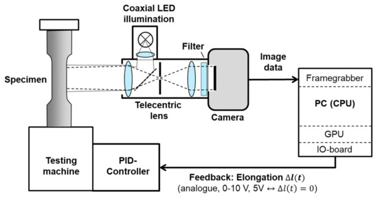
Figure 1.
Functional diagram of the closed-loop system. The digital image correlation (DIC) system delivers an analogue elongation signal so that it directly replaces a mechanical extensometer.
The algorithms were implemented using the C++ compiler shipped with Microsoft Visual Studio 2015 in combination with CUDA 8.0 programming SDK for the Nvidia GPU. The operating system was Microsoft Windows 7 64 Bit.
Figure 2 shows an image of the measurement head and an hourglass specimen mounted in a testing machine. Typical images recorded by this setup on polished hourglass specimen and the corresponding marker-free correlation images are shown in Figure 3.
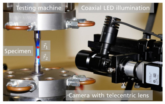
Figure 2.
Image of the DIC measurement head and of a polished specimen in a servo-hydraulic testing machine. The red crosses mark the template positions within the field-of-view.
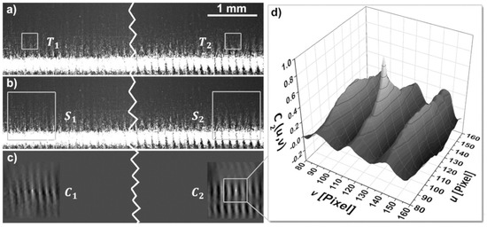
Figure 3.
Example images from a nickel-base superalloy (René 80) specimen: reference image (a) with template subsets , measurement image (b) with search subsets , zero-normalized cross-correlation results (c), and enlarged 3D graph of the right correlation peak (d). The images on the left (full size 2040 × 256 pixel) are split at the broken line.
2.2. Real-Time DIC Implementation
The starting point of the DIC algorithm implementation in C++/CUDA was the Matlab code given in [29]. However, this reference code uses the common aerial normalization, i.e., calculating mean and standard deviation over the whole subset area. For robust evaluation on cylindrical surfaces, all image subsets are normalized in a line-wise manner:
With , , and denoting the acquired pixel intensity, normalized intensity, average row intensity, and row standard deviation of either the template or the search image subsets, respectively. The indices and indicate the rows and columns within the template or search subsets. This normalization compensates the strong intensity drop with increasing angle of incidence which is in particular advantageous on polished cylindrical samples. Therefore, besides a well-adapted camera-lens combination, this normalization is a crucial step towards marker-free DIC measurements on polished surfaces. The normalized cross-correlation coefficient is calculated in Fourier space from the normalized and zero-padded template from the reference image and search subsets
In this equation, and denote row and column indices within the pixel correlation result and quantifies the template and search subsets within reference and search image (see Figure 3); the * denotes the complex conjugate. As it is normalized to the range of −1 to 1, values of near 1 indicate lag positions of great similarity between template and search subset, whereas values around zero indicate no similarity. Therefore, the maximum value marks the position of the template pattern with the accuracy of one pixel. However, the shape of the peak around the maximum is a direct consequence of the point-spread function of the optical system which means that it can be assumed as a constant pattern sampled by the image sensor [30]. This assumption leads to a subpixel evaluation of the peak position by fitting a polynomial to the 3 × 3 neighborhood of the maximum correlation at
One can also motivate this approach as a two-dimensional Taylor expansion of the peak. The coefficients correspond to the weighted derivatives and the subpixel-accurate peak position to the maximum of the fitted polynomial. The difference of the values for the position of template acquired at time yields the displacement with subpixel accuracy. The position vector is consequently calculated from the initial position , i.e., the center of the template , plus the displacement :
This algorithm is a rather straightforward implementation of the DIC problem sometimes referred to as fast Fourier transform-based cross-correlation (FFT-CC). It is path-independent with deterministic execution time and complexity if Equations (3) and (4) are executed on the GPU. Equation (5) describes a zero-order shape function measuring translation and disregarding shear and rotation—which is sufficient for 2D-DIC systems and typical fatigue strains in the range of 1%.
Figure 3 illustrates these evaluation steps. Images (a) and (b) are examples of a reference image with the templates and of a measurement image with search areas . The templates are positioned in the diffuse reflection area of the polished steel specimen. Although it looks quite specular, the surface exhibits a periodical structure caused by the polishing process. The cross-correlation results are given in image (c). The polishing structures cause some periodic noise, but on top there is a significant correlation peak originating from the incidental microstructure, i.e., the non-periodic patterns. On all investigated samples (steel, aluminum and nickel-base superalloys), this peak was sufficient for tracking the 3 × 3-pixel neighborhood enlarged in image (d) using a polynomial as given in Equation (5). Therefore, no further surface treating like the application of marker structures was necessary.
3. Results
3.1. Processing Time and Latency for Closed-Loop Control
To test the system’s performance, the average processing time of 1000 images in memory was measured for two subsets per image. To get the processing time for different steps, these steps were commented out measuring the difference in processing time. Figure 4 shows the result of the performance test for different correlation sizes measured for each processing step as described above. As soon as an image is acquired, CPU and GPU have to be synchronized by transferring the image subsets. In the second step, each subset is normalized on the GPU according to Equation (3). The third step covers Equation (4): the multiplication of the FFT transform of each search subset with the transformed image of the corresponding template subset from the first image and inverse FFT to obtain the cross-correlation result shown in Figure 3c. The final step comprises copying the 3 × 3 pixel neighborhood of back to the CPU and doing the subpixel-evaluation of the peak position according to Equations (5) and (6). The elongation between the two subsets is transformed into an analogue 0–10 V signal for the PID controller. All processing times given in Figure 4 are average processing times measured for 1000 images.
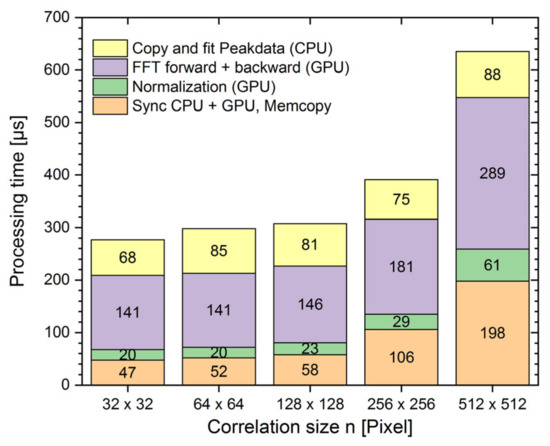
Figure 4.
Performance test results processing two subsets per image. The height of the bars gives the total processing time for two subsets per image, the numbers within each field give the processing time for each step in microseconds.
The processing times shown in Figure 4 are well below 800 microseconds, so they can be executed synchronously in a single thread running parallel to a second thread acquiring images from the camera with 1.2 kHz. Therefore, the latency of the system is the sum of the acquisition time for the camera image, the processing time given in Figure 4 and some latency for the DMA transfer to the analogue output. This assumption was confirmed by measuring the latency between the camera trigger signal and the analogue output with an oscilloscope. The result were 1.4 milliseconds for externally triggered image acquisition and 0.6 milliseconds for image processing. The resulting average dead time of the strain measurement is below 2 milliseconds.
Another important observation in Figure 4 is that the processing times rise only slowly with correlation size . For example, the total processing time for two subsets rises from 276 to 391 microseconds when the correlation size increases from 32 × 32 to 256 × 256 pixel because the synchronization of CPU and GPU as well as the organization on the GPU causes some significant overhead whereas the processing time is rather low. This makes it efficient on GPU-based systems to increase the search subset size instead of introducing additional algorithms for tracking. As discussed above, this increases the measurement robust against occasional mismeasurements.
3.2. Comparison to Mechanical Extensometer
In this section, the application of the developed measurement system is shown. For this purpose, tests were done with different materials under force control and closed-loop condition using a servo-hydraulic testing machine Instron 8502. Figure 5 shows the optically measured strain signal in comparison with the strain measured by a tactile extensometer (Maytec PMA-12/V7/1 [31]) for a force-controlled triangular cycle with a frequency of 10 Hz. The critical points for the closed-loop control in strain-controlled experiments are the turning points where the strain rate changes from positive to negative and vice versa. The optical sensor shows less noise than the mechanical sensor and pretty smooth transitions. Apparently, the bandwidth of the system is limited by the mechanics, not by the strain sensor measuring only 120 strain values per cycle–less than 400 as recommended by ASTM E606.
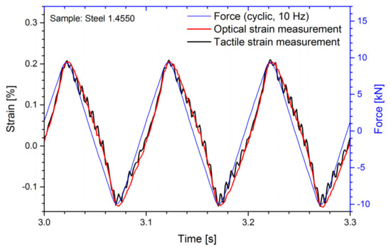
Figure 5.
Force-controlled test on austenitic steel 1.4550 at room temperature with a 10 Hz triangular force-controlled cycle. The optical system (red curve) resolves the turning points as well as the tactile mechanical extensometer (black curve).
As the system works marker-free, a calibrated digital dial gauge (Sylvac S_Dial Work Nano 2.5 mm [27]) was used to measure absolute elongation values. They were found to be in the range of ±0.5 micrometers, like the mechanical extensometer (Maytec PMA-12/V7/1 [31]). However, the calibration accuracy of the gauge was 0.38 micrometer (1σ). Therefore, the reproducibility of the elongation was measured in a ‘zero-strain-test’ where the specimen is moved without load. In this case, the reproducibility of the strain measurement was found to be in the range of 10−5 (1σ) with maximum and minimum in a range of ±3 × 10⁻⁵ [32]. So the measurement accuracy can be considered similar to the mechanical extensometer or optical ones based on IC-GN [5].
3.3. Strain-Controlled Testing
To ensure the applicability for high temperature material testing, a strain-controlled test was performed on nickel-base alloy René 80 at temperatures from 20 °C to 1000 °C. Stress–strain hysteresis combined with the change of the specimen surface are given in Figure 6. One recognizes the decreasing slopes of the curves corresponding to the decreasing elastic modulus of the material at increasing temperature. Near 1000 °C, the material becomes very soft and the stress–strain curves somehow deformed. This is not an artifact of the marker-free measurement, because similar behavior was observed after the application of markers.
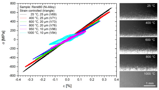
Figure 6.
Strain-controlled test on nickel-base alloy René 80 at different temperatures from room temperature to 1000 °C. The specimen surface changes with increasing temperature.
Dependent on the material chemical composition, some materials tend to form oxide layers on the surface at high temperatures, which can adversely affect the surface structure and thus the correlation quality. In Figure 6, the surface becomes darker with temperature increasing from room temperature to about 800 °C. This darkening is compensated by the normalization in Equation (3), making the correlation results comparable in this regime. At 1000 °C, oxidation is observable altering the specimen surface. The oxide itself was stable and the surface structure sufficient for marker-free measurements, but the altered structure is not comparable to that below 800 °C by correlation.
We also repeated the marker-free measurements from Figure 6 with a second speckle-painted sample as it is frequently used in DIC. Figure 7 shows stress–strain diagrams from both samples measured at 800 °C together with the corresponding camera images. The camera images of the marker-free measurement show a higher dynamics in vertical directions than the speckle-painted ones (Figure 7, right side). However, this dynamics in vertical direction is compensated by the line-wise normalization given in Equation (3). The camera we used has a dynamic range of 10 Bit (60 dB) which we found sufficient for measurements of ±20 degree from the specular reflex. As the inset shows, the noise was generally lower in the marker-free measurements. The reason for this noise reduction might be that the microstructure of sample exhibits structures on a broad range of spacial frequencies which is only limited by the resolution of the optics. So, the spectrum of these structures is closer to white noise then that of the speckle-painted structures despite their enlarged contrast. As a figure of merit, Young’s modulus was calculated for both measurements. With 162 GPa for the marker-free and 163 GPa for the speckle-painted measurement, it was quite similar. The algorithm described above works for both, marker-free and speckle painted samples.
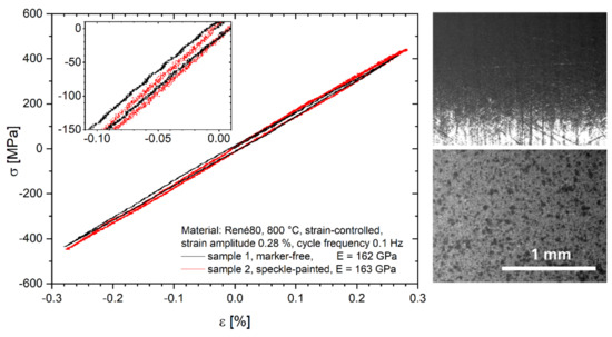
Figure 7.
Left: Strain-controlled stress–strain diagrams of a marker-free and a speckle-painted René80 samples. The inset shows the noise of both measurements. Right: Camera images from the marker-free sample 1 (top) and the speckle-painted sample 2 (bottom).
Classical strain-controlled fatigue tests with a duration of over 20 h were conducted to prove the stability of the system. Figure 8 shows the stress response of two experiments with identical conditions. It can be observed, that the resulting stress maxima are nearly the same. The cyclic loading of the specimen leads to crack initiation and crack propagation and thus to a reduction of the cross section which result in a stress drop at the end of the experiment. These cracks are often characterized by full-field strain measurements.
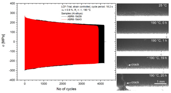
Figure 8.
Strain-controlled low cycle fatigue (LCF) tests on AlSi piston alloy for automotive applications. Crack propagation can be observed during the experiment.
Even if the shapes of the samples were similar, their surfaces however can differ greatly. Either by the manufacturing or by the machining process. Measurements on turned, polished, scratched, painted, and oxidized specimen surfaces showed good and reliable results.
3.4. Real-Time Strain-Field Measurement
Although the system is optimized for strain-controlled testing, it also allows for real-time strain-field measurement with a large number of subsets per image. Figure 9 shows an example measurement with 2500 subsets per image taken at the end of an LCF test after cracks appeared. As the trial was strain-controlled, it was straight forward to compare the image at maximum and minimum strain of within the same cycle.
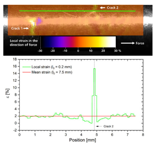
Figure 9.
Real-time strain-field measurement where the local displacement is superimposed by color to the camera image (top). Bottom: The green line shows local displacement with with a clear peak at crack 2. For strain-control, mean strain with of the green line is measured between the ends (red line in bottom graph).
Due to path-independency, it was possible to compare the minimum and maximum load images directly without need for the intermediate images at a correlation rate of 25 kHz or 10 full-field strain images per second. This rise in the correlation rate from 10 kHz in strain-controlled mode to 25 kHz because CPU and GPU are synchronized less frequently. If local strain is measured with a base length , cracks become clearly visible, as indicated by the green line. The line ends are the center positions of the two ROIs for mean strain measurement in strain control mode. The green line in the upper graph shows the image of the local strain profile given below. Obviously, there is a significant peak where the green line crosses crack 2.
This shows that the system should be good base for real-time extraction of crack parameters in future implementations. In particular, strain-field measurement can be combined with strain-control to extract strain-field at minimum and maximum load in real-time. This means that the system does not only replace the mechanical extensometer and the optical strain-field measurement, it also adds some synergy by ‘load synchronized measurement’.
4. Discussion
4.1. Sampling Rate and Processing Speed
This article reports a 2D-DIC system especially optimized for strain-controlled LCF testing. This closed-loop control application requires a high sampling rate above 1 kHz and a low latency in the range of a few milliseconds. Both requirements are quite hard to meet for image processing systems. Robustness is an issue because a small number of mismeasurements can already cause critical fluctuations in the feedback signal leading to specimen failure. On the other hand, the deformations of the specimen at LCF is rather small–in the range of 1%-so that rotation and shear deformations are negligible. To achieve a low latency, we chose a ‘fast and simple’ FFT-CC implementation neglecting shear and rotation, because it does not require iterative calculations like the more common IC-GN algorithm. As strain-control requires only a minimum of two measurement positions per image, the FFT-CC approach allows for a fast and path-independent implementation if the search field size is sufficient to measure the maximum displacement in a single step. Here, the FFT-CC approach benefits in particular from the GPU architecture where the FFT calculation is of the complexity . IC-GN, on the contrary, relies on a good initial guess, which is good if temporal or spatial neighborhood can be exploited–like in typical strain field applications with small displacement steps between subsequent images.
To quantify these effects, Table 2 compares these parameters for some fast 2D-DIC implementations. Pan et al. [33] published a highly speed-optimized CPU implementation based on the IC-GN algorithm processing almost 30,000 template subsets of 21 × 21 pixel in 0.685 s—which corresponds a processing rate of 44 kHz. As the system is CPU-based, this processing rate varies strongly with template size. For 61 × 61 pixel per subset, the processing rate decreases to 7.2 kHz. A year later, the same authors published a real-time extensometer measuring four templates per image at a frame rate of 117 Hz, i.e., a processing rate of 0.468 kHz [5]. This decrease shows how much the IC-GN implementation exploits the neighborhood of the full-field measurement. This processing rate is quite comparable to the 0.6 kHz we measured for our approach without using the GPU. Wang et al. thoroughly studied different combinations of both algorithms implemented on CPU and GPU. Variation 2 was the fastest path-depending full-field implementation whereas variation 4 achieved the highest real-time processing rate in a path-independent way. Here, the path-dependent tracking increased the processing rate from 3 to 283 kHz.
Table 2.
Performance comparison of different real-time 2D-DIC systems. Parameters marked with ‘-‘ are not provided in the corresponding publication.
The processing rate of 9.6 kHz that we achieved in strain-controlled mode is faster than the 3 kHz published by Wang [22] for the path-independent variation 4 and it outperforms the CPU-based real-time extensometer by Pan [5] by more than an order of magnitude. In full-field mode, the processing rate of our system increases to 25 kHz, but it might be outperformed by an order of magnitude if tracking is allowed. In contrast to tracking based systems, where the maximum displacement is only limited by the field-of-view, our approach has a hard limit for the maximum displacement .
4.2. Latency
None of the other publications provides values for the latency although that is a very important parameter for PID controlled closed-loop applications. As the camera frame rate plus processing time form a lower boundary for the latency of image processing systems, it is obvious that it must be longer than the 2 ms of our approach in all cases. This is also true for the commercial systems by Correlated Solutions [34], Instron [4], and Zwick Roell [35] with frame rates of 250, 490, and 160 Hz, respectively. Unfortunately, none of these companies specifies the conditions necessary to achieve these sampling rates. In our case, the image processing adds only 0.6 ms to the image reading time which is quite at the lower boundary of what preemptive multitasking systems like Windows require without GPU. Therefore, there is no significant additional latency due to the GPU. Shorter latencies for image processing systems in the range of 0.1 ms require different hardware architectures like FPGA or specialized sensor-processor hardware like cellular neural networks [26,36].
4.3. Marker-Free Measurement
In addition to high processing rate and short latency, our system also provides marker-free DIC measurement on polished metals at a rather large field-of-view of more than 10 mm. This avoids a second disadvantage common for most current DIC systems: the need for specimen preparation. Besides the additional work, markers or speckle-paint can break or delaminate during the experiment. In addition, the markers have to withstand experimental conditions like high temperatures, and they must create unique patterns on a scale suitable for correlation. Characteristic surface (marker) generation is possible but requires certain experience and might not be allowed for industrial processes.
According to our experience with polished specimen from aluminum, nickel-based superalloys and steel, the incidental microstructure exhibits patterns on multiple scales which are well suited for correlation. Generally, we found the noise on polished metal specimen to be lower measuring marker-free rather than using speckle-paint, presumably because the incidental microstructure of the sample surfaces exhibited a wider range of spacial frequencies allowing to exploit the full resolution of the optics. Critical are periodic structures on the specimen surface originating from polishing processes because they create non-statistical noise in the correlation result. Their impact on the sub-pixel displacement measurement was eliminated by filtering the images with a Gaussian low-pass filter.
The reproducibility of the marker-free strain measurement was a standard deviation of 10−5 (1σ) and a maximum error of ±3 ×·10−5 measured by a zero-strain-test [32]. It is similar to that of IC-GN based system of Pan et al. [5] quantified by self-consistency using Poisson’s ratio. In our case, the camera resolution is larger (2048 pixel with 61 × 61 pixel per subset instead of 1024 pixel with 41 × 41-pixel subsets in [5]) and the subpixel-resolution lower (0.02 pixel instead of 0.005) which might be an effect of the zero-order shape function. However, these values are not exactly comparable. Nevertheless, they give a hint because other references are hardly available.
5. Conclusions
This article reports a GPU-based path-independent video extensometer with two major novelties: First, it achieves sampling rates of 1.2 kHz, which is close to mechanical extensometers, and the analogue strain signal is generated with a latency of 2 milliseconds. Therefore, it is able to replace mechanical extensometers in standard LCF testing machines fulfilling the recommendations of ASTM E606 for standard strain-controlled fatigue testing with cycle frequencies up to 3 Hz. According to our knowledge, this is one of the first GPU-based image processing systems for real-time closed-loop applications. Second, it enables marker-free DIC measurements on polished hourglass specimen without loss of accuracy. As it is also able to acquire full-field strain images, this sensor combines most advantages of state-of-the-art optical and mechanical extensometers in terms of sampling rate, non-tactile and slip-free measurement, and full-field strain acquisition. Therefore, it simplifies LCF testing and it might trigger many new applications, in particular, if strain-fields need to be acquired synchronously to the load. It might also trigger industrial applications because the marker-free operation eliminates the need for sample preparation.
Author Contributions
Conceptualization, D.C. and C.E.; Funding acquisition, A.B., and M.S; Investigation, D.J.R., S.E., and M.S.; Methodology, A.B., S.E., and M.S.; Project administration, A.B., M.S., and S.E.; Software, A.B. and D.J.R.; Supervision, A.B.; Writing—original draft, A.B. and S.E.; Writing—review and editing, D.J.R., M.S., A.B. and D.C.
Funding
This research was funded by the Fraunhofer-Gesellschaft in the project ‘Schnelle und berührungslose optische Dehnungsmessung zur Echtzeit-Regelung bei der Materialprüfung »StrainControl«’.
Conflicts of Interest
The authors declare no conflict of interest.
References and Notes
- ASTM E606/606M: Standard Test Method for Strain-Controlled Fatigue Testing; ASTM International: West Conshohocken, PA, USA, 2012.
- Kanchanomai, C.; Yamamoto, S.; Miyashita, Y.; Mutoh, Y.; McEvily, A.J. Low cycle fatigue test for solders using non-contact digital image measurement system. Int. J. Fatigue 2002, 24, 57–67. [Google Scholar] [CrossRef]
- Zhang, S.; Mao, S.; Arola, D.; Zhang, D. Characterization of the strain-life fatigue properties of thin sheet metal using an optical extensometer. Opt. Lasers Eng. 2014, 60, 44–48. [Google Scholar] [CrossRef]
- Bailey, P.; Higham, M. Application of strain-controlled fatigue testing methods to polymer matrix composites. Procedia Struct. Integr. 2016, 2, 128–135. [Google Scholar] [CrossRef][Green Version]
- Pan, B.; Tian, L. Advanced video extensometer for non-contact, real-time, high-accuracy strain measurement. Opt. Express 2016, 24, 19082–19093. [Google Scholar] [CrossRef] [PubMed]
- Halama, R.; Gál, P.; Paška, Z.; Sedlák, J.; Vasko, M.; Handrik, M.; Jakubovičová, L.; Kopas, P.; Blatnická, M.; Baniari, V.; et al. A new accelerated technique for validation of cyclic plasticity models. MATEC Web Conf. 2018, 157, 05008. [Google Scholar] [CrossRef][Green Version]
- Unbehauen, H.; Ley, F. Regelungs- und Steuerungstechnik. In HÜTTE—Das Ingenieurwissen, 34th ed.; Czichos, H., Ed.; Springer: Berlin/Heidelberg, Germany, 2012. [Google Scholar]
- Kamaya, M.; Kawakubo, M. Mean stress effect on fatigue strength of stainless steel. Int. J. Fatigue 2015, 74, 20–29. [Google Scholar] [CrossRef]
- Eckmann, S.; Schweizer, C. Characterization of fatigue crack growth, damage mechanisms and damage evolution of the nickel-based superalloys MAR-M247 CC (HIP) and CM-247 LC under thermomechanical fatigue loading using in situ optical microscopy. Int. J. Fatigue 2017, 99, 235–241. [Google Scholar] [CrossRef]
- Gupta, S.; Beaudoin, A.J.; Chevy, J. Strain rate jump induced negative strain rate sensitivity (NSRS) in aluminum alloy 2024. Experiments and constitutive modeling. Mater. Sci. Eng. 2017, 683, 143–152. [Google Scholar] [CrossRef]
- Johanson, A.; Viespoli, L.M.; Nyhus, B.; Alvaro, A.; Berto, F.; Hénaff, G. Experimental and numerical investigation of strain distribution of notched lead fatigue test specimen. MATEC Web Conf. 2018, 165, 05003. [Google Scholar] [CrossRef]
- Pan, B.; Wu, D.; Wang, Z.; Xia, Y. High-temperature digital image correlation method for full-field deformation measurement at 1200 °C. Meas. Sci. Technol. 2011, 22, 015701. [Google Scholar] [CrossRef]
- Berke, R.B.; Lambros, J. Ultraviolet digital image correlation (UV-DIC) for high temperature applications. Rev. Sci. Instrum. 2014, 85, 045121. [Google Scholar] [CrossRef]
- Blaber, J.; Adair, B.S.; Antoniou, A. A methodology for high resolution digital image correlation in high temperature experiments. Rev. Sci. Instrum. 2015, 86, 035111. [Google Scholar] [CrossRef]
- Gianola, G.S.; Eberl, C. Micro- and nanoscale tensile testing of materials. JOM J. Miner. Met. Mater. Soc. 2009, 61, 24. [Google Scholar] [CrossRef]
- Pan, B.; Qian, K.; Xie, H.; Asundi, A. Two-dimensional digital image correlation for in-plane displacement and strain measurement. A review. Meas. Sci. Technol. 2009, 20, 062001. [Google Scholar] [CrossRef]
- Schreier, H.; Orteu, J.J.; Sutton, M.A. Image Correlation for Shape, Motion and Deformation Measurements; Springer: Boston, MA, USA, 2009; Chapter 5.5; p. 99. [Google Scholar]
- Xavier, J.; Sousa, A.M.R.; Morais, J.J.L.; Filipe, V.M.J.; Vaz, M. Measuring displacement fields by cross-correlation and a differential technique: Experimental validation. Opt. Eng. 2012, 51, 043602. [Google Scholar] [CrossRef]
- Goos, G. Paralleles Rechnen und Nicht-Analytische Lösungsverfahren; Springer: Berlin, Germany, 1998. [Google Scholar]
- Lu, P.J.; Oki, H.; Frey, C.A.; Chamitoff, G.E.; Chiao, L.; Fincke, E.M.; Foale, C.M.; Magnus, S.H.; McArthur, W.S.; Tani, D.M.; et al. Orders-of-magnitude performance increases in GPU-accelerated correlation of images from the International Space Station. J. Real Time Image Proc. 2010, 5, 179–193. [Google Scholar] [CrossRef]
- Zhang, L.; Wang, T.; Jiang, Z.; Kemao, Q.; Liu, Y.; Liu, Z.; Tang, L.; Dong, S. High accuracy digital image correlation powered by GPU-based parallel computing. Opt. Lasers Eng. 2015, 69, 7–12. [Google Scholar] [CrossRef]
- Wang, T.; Kemao, Q.; Seah, H.S.; Lin, F. A flexible heterogeneous real-time digital image correlation system. Opt. Lasers Eng. 2018, 110, 7–17. [Google Scholar] [CrossRef]
- Thiagu, M.; Subramanian, J.S.; Nasre, R. Fast, sub-pixel accurate digital image correlation algorithm powered by heterogeneous (CPU-GPU) framework. In Advancement of Optical Methods & Digital Image Correlation in Experimental Mechanics; Conference Proceedings of the Society for Experimental Mechanics Series; Lamberti, L., Lin, M., Furlong, C., Sciammarella, C., Reu, P.L., Eds.; Springer: Cham, Switzerland, 2019; p. 3. [Google Scholar]
- Gautier, N.; Aider, J.L. Real-time planar flow velocity measurements using an optical flow algorithm implemented on GPU. J. Vis. 2015, 18, 277–286. [Google Scholar] [CrossRef]
- Nakabo, Y.; Ishikawa, M.; Toyoda, H.; Mizuno, S. 1 ms column parallel vision system and its application of high speed target tracking. In Proceedings of the 2000 ICRA Millennium Conference, IEEE International Conference on Robotics and Automation, San Francisco, CA, USA, 24–28 April 2000; Volume 1, pp. 650–655. [Google Scholar]
- Blug, A.; Abt, F.; Nicolosi, L.; Heider, A.; Weber, R.; Carl, D.; Höfler, H.; Tetzlaff, R. The full penetration hole as a stochastic process: Controlling penetration depth in keyhole laser-welding processes. Appl. Phys. B 2012, 108, 97–107. [Google Scholar] [CrossRef]
- Sylvac Switzerland Crissier, Chemin du Closalet 16, 1023 Crissier, Switzerland
- Sutton, M.A.; Yan, J.H.; Tiwari, V.; Schreier, H.W.; Orteu, J.J. The effect of out-of-plane motion on 2D and 3D digital image correlation measurements. Opt. Lasers Eng. 2008, 46, 746–757. [Google Scholar] [CrossRef]
- Digital Image Correlation and Tracking. Available online: https://uk.mathworks.com/matlabcentral/fileexchange/50994-digital-image-correlation-and-tracking (accessed on 6 April 2019).
- Goodman, J.W. Introduction to Fourier Optics, 2nd ed.; McGraw-Hill: New York, NY, USA, 1996. [Google Scholar]
- MAYTEC Mess- und Regeltechnik GmbH, Im Haselbusch 16, D-78224 Singen, Germany
- Blug, A.; Regina, D.J.; Eckmann, S.; Senn, M.; Bertz, A.; Carl, D.; Eberl, C. GPU-based digital image correlation system for real-time strain-controlled fatigue and strain field measurement. In Proceedings of the SPIE 2019, 11056-30, Optical Metrology Conference, Munich, Germany, 24–27 June 2019. [Google Scholar]
- Pan, B.; Tian, L. Superfast robust digital image correlation analysis with parallel computing. Opt. Eng. 2015, 54, 034106. [Google Scholar] [CrossRef]
- VIC-Gauge Real-Time Strain Measurement. Specifications VIC-2D 6; Correlated Solutions, Inc.: Irmo, SC, USA. Available online: https://www.correlatedsolutions.com/wp-content/uploads/2014/04/VIC-Gauge-2D-System-Specs.pdf (accessed on 6 April 2019).
- VideoXtens 2-120 HP-High Precision without Contacting; ZwickRoell GmbH & Co. KG: Ulm, Germany. Available online: https://www.zwickroell.com/-/media/files/sharepoint/vertriebsdoku_pi/08_893_videoxtens_2-120_hp_pi_d.pdf (accessed on 6 April 2019).
- Nicolosi, L.; Blug, A.; Abt, F.; Tetzlaff, R.; Höfler, H.; Carl, D. Real time control of laser beam welding processes-reality. In Focal-Plane Sensor-Processor Chips, 1st ed.; Zarándy, A., Ed.; Springer Science+Business Media LLC: New York, NY, USA, 2011. [Google Scholar]
© 2019 by the authors. Licensee MDPI, Basel, Switzerland. This article is an open access article distributed under the terms and conditions of the Creative Commons Attribution (CC BY) license (http://creativecommons.org/licenses/by/4.0/).