A Neural Network Based Sliding Mode Control for Tracking Performance with Parameters Variation of a 3-DOF Manipulator

Featured Application

The proposed control scheme can be applied not only for position tracking control for industrial manipulators, but also for any non-linear systems to improve its performance.

Abstract

The manipulator, in most cases, works in unstructured and changeable conditions. With large external variations, the demand for stability and robustness must be ensured. This paper proposes a neural network sliding mode control (NNSMC) to cope with uncertainties and improve the behavior of the robotic manipulator in the presence of an external disturbance. The proposed method is applied to the three degrees of freedom (DOF) manipulator. Some comparisons between the proposed and the conventional algorithms are given in both simulation and experiments to prove that the designed control can achieve higher accuracy in tracking motion.

1. Introduction

In recent years, robot manipulators have been rapidly developing in many applications that require high accuracy in tracking performance. However, up to now, formulating controllers satisfying control performance and the stability of the system is still a big challenge due to its high nonlinearity, coupling dynamics reactions, and uncertainties [1]. In order to deal with these problems, many approaches such as using a proportional integral derivative (PID) control [2], feedback linearization [3], robust control [4,5], adaptive control [6,7,8], backstepping (BSP) control [9,10], hybrid proportional derivative sliding mode control (PDSMC) [11], sliding mode control (SMC) [12,13,14,15] and even intelligent control [16,17,18,19,20,21,22,23,24,25,26,27,28,29,30,31] have been studied.

Sliding mode control (SMC) is known as one of the most feasible solutions with fast response and strong robustness to resolve perturbation such as external disturbances, or unmodeled blocks in nonlinear systems compared with traditional methods [14,15]. When precise control is considered as an important criterion, the adaptive algorithm needs to be constructed rigorously. Ahmed et al. [16] formulated an adaptive fuzzy sliding mode control (AFSMC) using a supervisory fuzzy control where a fuzzy logic system (FLS) was employed to replace switching terms and switching gain in the robust control signal of the SMC. Jun et al. [17] integrated adaptive laws to determine the parameters of the FLS and then used FLS to approximate switching gains and eliminate the chattering. The FLS, whose laws were designed based on some knowledge about the control system [18], has been successfully applied to many linear and non-linear systems [19,20]. In such studies, the FLS with adaptive laws were employed to adjust controller gains of the SMC. The adjusted gains for the controller were chosen based on trial-and-error methods and experiments to determine suitable values. Those results indicated that the tracking performance could be improved. However, as mentioned above, the FLS was set up based on the knowledge of the system dynamics and experience of designers, which is difficult to carry out in practice, and the matrix of fuzzy rules is complicated to design [21].

Neural network control (NN) has been successfully used in many commercial and industrial applications in recent years [21,22,23,24,25,26,27,28,29,30,31]. In those studies, the NN is used as a compensator or an approximator to boost or enhance the control signal, compensate uncertainties, or eliminate disturbances. Tairen et al. employed the NN to observe the velocity of links and then combined with an adaptive law and SMC to compensate for errors and disturbance [22]. Tran et al. used radial basis function (RBF) NN to estimate system dynamics and compensate approximation errors as well [23]. Seul proposed a reference compensation technique (RCT) where the NN was constructed to compensate uncertainties at the trajectory level [24,25]. Vo. et al. proposed the radial basis function neural network (RBFNN) to approximate unknown robot function [26]. To et al. utilized RBFNN to control the position of a piezo positioning stage [27]. Vu et al. proposed a robust adaptive control method based on a dynamic structure fuzzy wavelet neural network (FWNNs) system for trajectory tracking control of industrial robot manipulators to compensate for structured and unstructured uncertainties and to model complex processes [28]. These results indicated that the tracking performance was improved compared with the conventional technique. Besides that, the NN technique can be used to directly adjust the controller to adapt to the system dynamics. Some approaches utilized this technique for adjusting the controller gains to achieve higher performance [21,29,30,31]. Tu et al. exploited the NN using the back-propagation method to fine-tune the PID gains to improve the tracking performance of the 2 degree of freedom (DOF) pneumatic artificial muscle (PAM) [21]. Ahn et al. proposed a switching algorithm for tuning PID gains using a learning vector quantization neural network to achieve accurate position control under the change of external payload [29]. Le et al. considered nonlinear PD computed torque in which the proportional and derivative gains were tuned to minimize the cost function [31].

Different from the FLS, the NN technique uses adaptive laws to minimize the cost function. The convergence of error depends on learning rates. However, no results using NN have been reported to adjust directly the controller gains of the SMC to improve the system performance. Most of the previous articles focused primarily on estimating and compensating uncertainties. Besides, in those previous studies, initial gains of the controller or suitable values of the parameters as well as the slope of the sliding surface were not discussed clearly.

Motivated by previous works and in an effort to improve and achieve high tracking performance in the action of external disturbance, a neural network sliding mode control (NNSMC), where the NN is used to directly adjust the controller gains of the sliding mode control (SMC), is proposed to overcome the problem of payload variation for a 3-DOF manipulator. We basically come up with an idea of using back-propagation for updating parameters to adapt to variable working conditions. Not only the robust gains are fine-tuned, but also the slopes of the sliding surfaces are adjusted in order to reduce system tracking errors. Some simulated results and experiments are given to verify an improvement and effectiveness of the proposed control in tracking performance in the presence of an external payload.

This paper is organized as follows: Section 2 presents the manipulator dynamics. The motion of the manipulator dynamics is discussed in this section. The proposed algorithm for the system is designed in Section 3. Some simulations are given in Section 4. In Section 5, we discuss the hardware setup for the test bench and some experiments are carried out to verify the proposed algorithm. Conclusions and future work are discussed in Section 6.

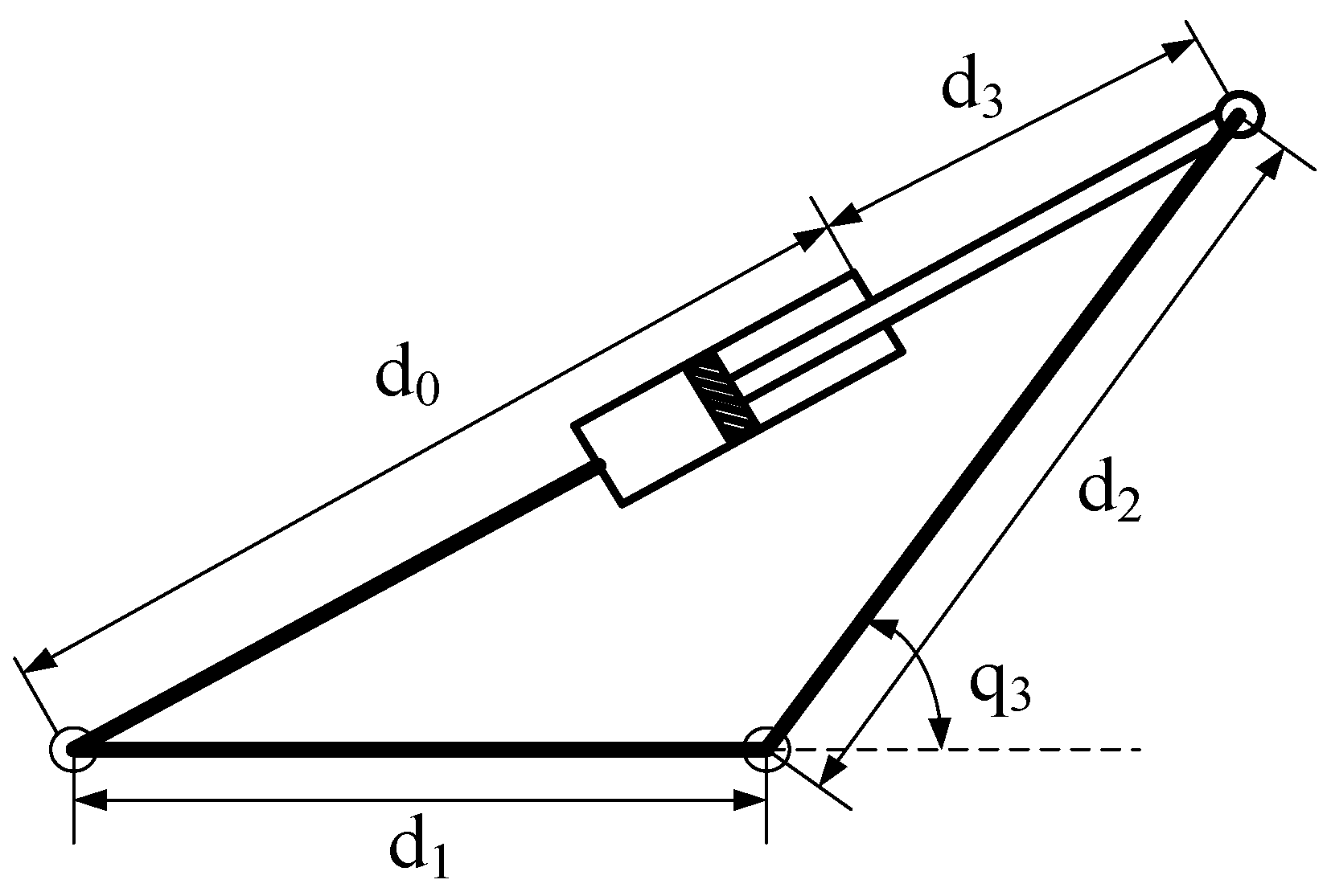
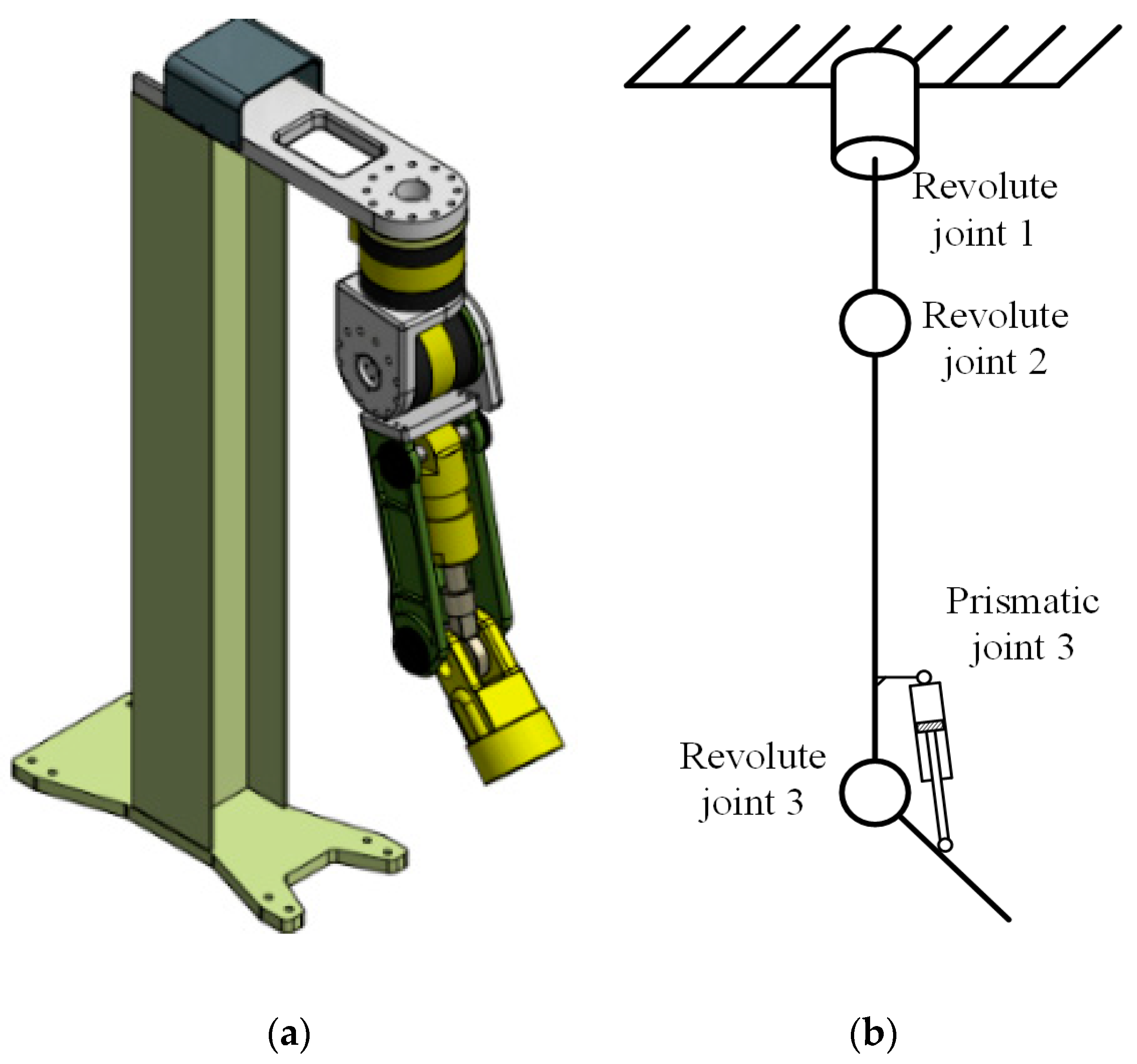
2. Manipulator Dynamics

The structure of the 3-DOF manipulator is described in Figure 1.

The dynamics of the 3-DOF can be expressed as:

$$M(q)\ddot{q}+C(q,\dot{q})\dot{q}+G(q)+F_d\dot{q}+F_s\left(\dot{q}\right)=\tau$$

(1)

where $q,\dot{q},\ddot{q}\in R^3$ are position, angular velocity, and angular acceleration vectors of each joint, respectively, $M(q)\in R^{3\times 3}$ is the symmetric and positive definite matrix of inertia, $C(q,\dot{q})\in R^{3\times 3}$ denotes the Coriolis and centrifugal term matrix, $G(q)\in R^3$ is the gravity term, τ is torque acting on joints, $F_d\in R^{3\times 3}$ is a diagonal matrix of viscous and dynamic friction coefficients, and $F_s\in R^3$ is the vector of unstructured friction effects such as static friction terms.

In practice, the dynamics of the manipulator is difficult to determine clearly due to the mass distribution, and oscillation in the process of operation. Then the Equation (1) is represented as follows:

$$\widehat{M}(q)\ddot{q}+\widehat{C}(q,\dot{q})\dot{q}+\widehat{G}(q)+{\tau }_d=\tau$$

(2)

where $\widehat{M}(q)\ddot{q}+\widehat{C}(q,\dot{q})\dot{q}+\widehat{G}(q)$ represents the estimated terms of $M(q)\ddot{q}+C(q,\dot{q})\dot{q}+G(q)$, and can be assumed to be known, and ${\tau }_d=\Delta M(q)\ddot{q}+\Delta C(q,\dot{q})\dot{q}+\Delta G(q)+F_s\left(\dot{q}\right)+F_d\dot{q}\in R^3$ is the vector of any generalized input due to uncertainties, disturbances or un-modeled terms.

Assumption. 

All$\Delta (.)$are supposed to be bounded, i.e.,${\Vert \Delta (.)\Vert }_{\infty }\le \xi (.)$.

Unlike a conventional manipulator, the last link of our proposed hydraulic manipulator employs a cylinder to load heavier objects. The torque acting on the joint is essentially induced by force generated by the cylinder; then the relationship between the rotational motion of the joint and the translational motion of the actuator will be investigated. The architecture of the last link is illustrated in Figure 2.

The correlation between the motion of the actuator in the actuator space and the motion in joint space can be derived by:

$$d_0+d_3=\sqrt{d_1{}^2+d_2{}^2-2d_1{d}_2\cos \left(\pi -q_3\right)}$$

(3)

where $d_0$ is an initial length in case of maximum retracting; the positive direction in the actuator space is chosen for extracting the piston. $d_3$ denotes the position of the end-effector under the motion of the cylinder, $d_1$ and $d_2$ are fixed length of the hinge joints.

To obtain the correlational velocity between the actuator and the joint motion, taking the derivation respect to time, the Equation (3) is:

$${\dot{d}}_3=\frac{\partial d_3}{\partial q_3}{\dot{q}}_3=\frac{d_1{d}_2\sin \left(\pi -q_3\right)}{\sqrt{d_1{}^2+d_2{}^2-2d_1{d}_2\cos \left(\pi -q_3\right)}}{\dot{q}}_3=J_{a3}\left(q_3\right){\dot{q}}_3$$

(4)

where J_a3 (q3) is a Jacobian matrix of the 3^rd joint.

Thus, a torque acting on this joint can be derived as:

$${\tau }_3=J_{a3}^T\left(q_3\right)F_3.$$

(5)

The completely correlational motion between the actuator and the joint motion is described by:

$$\left(\begin{array}{c}{\dot{q}}_{1a}\\ {\dot{q}}_{2a}\\ {\dot{d}}_3\end{array}\right)=\left(\begin{array}{ccc}1& 0& 0\\ 0& 1& 0\\ 0& 0& J_{a3}\left(q_3\right)\end{array}\right)\left(\begin{array}{c}{\dot{q}}_1\\ {\dot{q}}_2\\ {\dot{q}}_3\end{array}\right)$$

(6)

where ${\left(\begin{array}{ccc}{q}_{1a}& q_{2a}& d_3\end{array}\right)}^T\in R^3$ denotes a position vector of the actuator in actuator space.

3. Controller Design

3.1. Sliding Mode Control

Define error variables such as:

$$e=q-q_d\in R^3,\dot{e}=\dot{q}-{\dot{q}}_d\in R^3,\ddot{e}=\ddot{q}-{\ddot{q}}_d\in R^3$$

(7)

where $e\in R^3$ is the error between the desired position and a simulated position, $q_d,{\dot{q}}_d,{\ddot{q}}_d\in R^3$ are the vector of the desired position, desired angular velocity, and desired angular acceleration of the joint, respectively, and $e\hspace{0.17em}\mathrm{and}\hspace{0.17em}\dot{e}$ are supposed to be bounded. Then the sliding surface s(t) in the state–space $R^3$ can be derived as:

$$s={\left(\frac{d}{dt}+\lambda \right)}^{n-1}e$$

(8)

where $\lambda =diag\left(\begin{array}{ccc}{\lambda }_1& {\lambda }_2& {\lambda }_3\end{array}\right),\hspace{0.17em}{\lambda }_i\hspace{0.17em}\left(i=1,2,3\right)$ is a positive constant.

In this circumstance, we choose n = 2, i.e., $s=\dot{e}+\lambda e$ is a function of the tracking position error and the velocity error based on the manipulator dynamics.

The derivative of the sliding surface with respect to time is derived as:

$$\dot{s}=\ddot{e}+\lambda \dot{e}\hspace{0.17em}={\widehat{M}}^{-1}(q)\left[\tau -\widehat{C}(q,\dot{q})\dot{q}-\widehat{G}(q)-d\right]-{\ddot{q}}_d+\lambda \left(\dot{q}-{\dot{q}}_d\right).$$

(9)

Property. 

$\dot{\widehat{M}}(q)-2\widehat{C}(q,\dot{q})$is a skew matrix that satisfies with$x^T\left[\dot{\widehat{M}}(q)-2\widehat{C}(q,\dot{q})\right]x=0$for any vector$x\in R^n$. Then, multiplying both sides of the equation above with$M(\theta )$, we obtain:

$$\widehat{M}\dot{s}=\widehat{M}\left(\ddot{e}+\lambda \dot{e}\right)\hspace{0.17em}=\tau -\widehat{C}(\dot{q},q)\dot{q}-\widehat{G}(q)-\widehat{M}(q){\ddot{q}}_d+\widehat{M}(q)\lambda \dot{e}+d.$$

(10)

The Lyapunov function can be defined as:

$$V=\frac{1}{2}{s}^T\widehat{M}s.$$

(11)

Taking the derivative, the Equation (11) with respect to time, we obtain:

$$\dot{V}=s^T\left[\tau -\widehat{C}(q,\dot{q})\left({\dot{q}}_d-\lambda e\right)-\widehat{G}(q)-\widehat{M}\left(q\right)\left({\ddot{q}}_d-\lambda \dot{e}\right)+d\right].$$

(12)

Let the equivalent state ${\dot{q}}_s=\dot{q}-s={\dot{q}}_d-\lambda e\to \hspace{0.17em}{\ddot{q}}_s=\ddot{q}-\dot{s}={\ddot{q}}_d-\lambda \dot{e}$ [18]; then substituting into Equation (8), we obtain:

$$\dot{V}=s^T\left[\tau -\widehat{C}(q,\dot{q}){\dot{q}}_s-\widehat{G}(q)-\widehat{M}\left(q\right){\ddot{q}}_s+d\right].$$

(13)

Then the control signal function is designated as:

$${\tau }_{control}=\widehat{C}(q,\dot{q}){\dot{q}}_s+\widehat{G}(q)+\widehat{M}\left(q\right){\ddot{q}}_s-\alpha \tanh (s)-Ks$$

(14)

where $\alpha =diag\left(\begin{array}{ccc}{\alpha }_1& {\alpha }_2& {\alpha }_3\end{array}\right)$ is a diagonal positive definite matrix, α_i is positive constant, $\tanh (s)={\left(\begin{array}{ccc}\tanh (s_1)& \tanh (s_2)& \tanh (s_3)\end{array}\right)}^T$, and K = diag(K₁, K₂, K₃) is a positive matrix in which $\hspace{0.17em}{s}^{T}Ks>0\hspace{0.17em}\hspace{0.17em}\forall \hspace{0.17em}s\ne 0$. The term –Ks is added to force the state to approach the switching manifolds faster and the tracking error will be converged in a finite time.

The stability of the system can be easily proved if the gains of the switching controller are bigger than the upper bounded uncertainties. Then substituting Equation (14) to (13), one can obtain:

$$\dot{V}\hspace{0.17em}=-s^T\alpha \tanh (s)-s^{T}Ks+s^{T}d.$$

(15)

Since we supposed that all $\Delta (.)$ are bounded, i.e.,${\Vert d\Vert }_{\infty }\le d_{bound}$, then to guarantee the stability of the system, the derivative of the Lyapunov function must be negative:

$$\dot{V}\hspace{0.17em}\le -s^T\alpha \tanh (s)-s^{T}Ks+s^T{d}_{bound}\le 0$$

(16)

$$\to s^T\alpha \tanh (s)+s^{T}Ks\ge s^T{d}_{bound}$$

(17)

where $d_{bound}=f\left(\dot{x}\right)=f_1\dot{x}+f_{2}sign(\dot{x})$ and f₁ and f₂ are positive constant matrices.

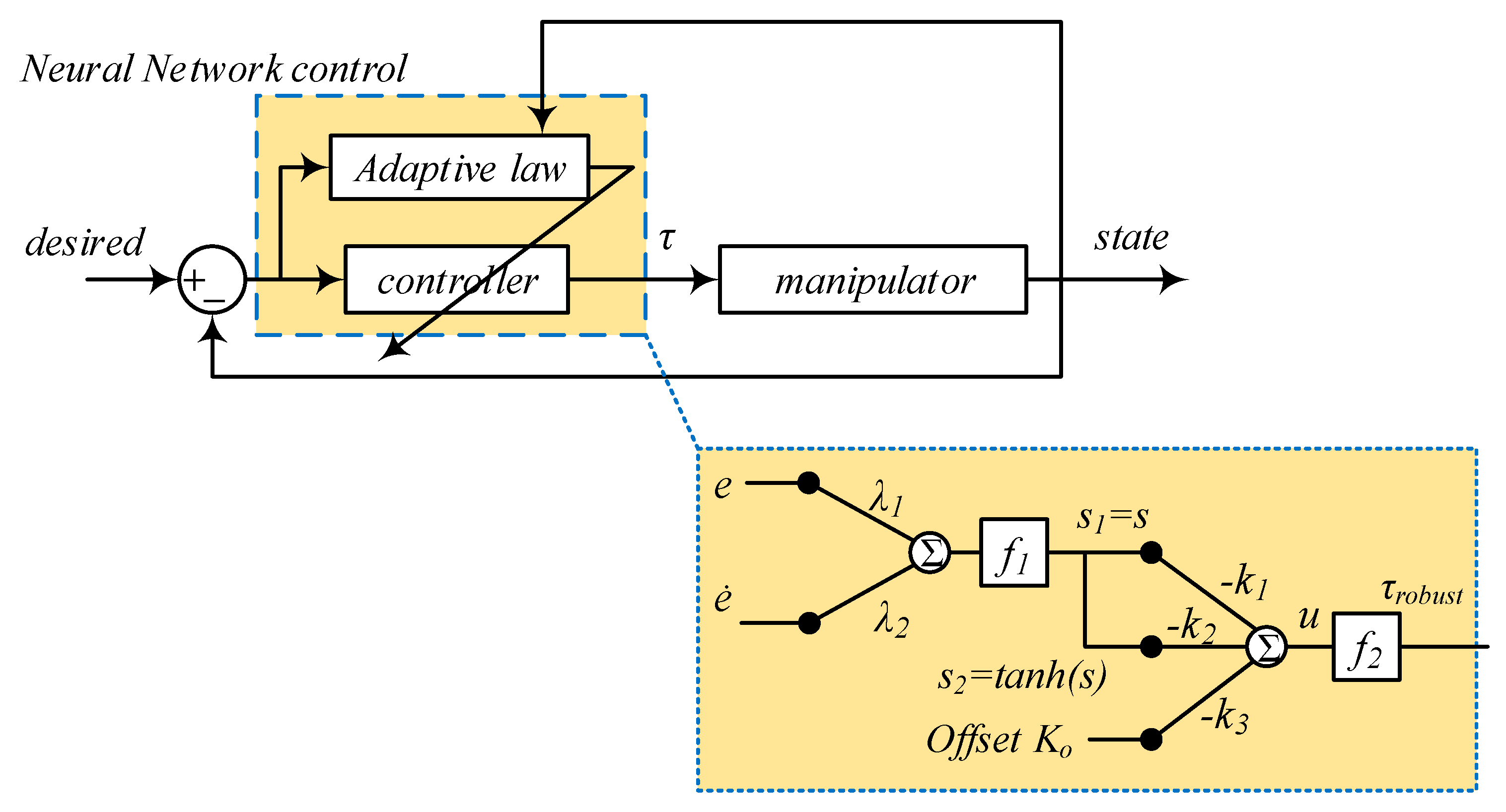
3.2. Neural Network Control

According to the portrait phase of the sliding mode control presented in Yuri et al. [32] and Wilfrid [33], the first stage is when the state trajectory is outside the sliding surface and needs to be driven towards the sliding surface. Then the second phase occurs when the state trajectory moves along towards the sliding surface. The term $-\alpha \tanh (s)-Ks$ in Equation (14) is to drive the state trajectory toward the sliding surface, whereas the slope λ of the sliding surface affects the convergence of state variables. The two-terms λ and robust term $-\alpha \tanh (s)-Ks$, in fact, depend on each other. The correlation between the two terms is depicted in Figure 3.

Despite the robustness of the sliding mode control, the tracking performance is difficult to achieve with high precision with fixed robust gains in the presence of the external payload. Some articles have reported the algorithm for gains-tuning using the neural network method. In this part, the neural network based sliding mode control is designed to adapt with the parameter variation. The NNSMC architecture is described in Figure 4.

As can be seen in Figure 4, instead of setting the fixed value for both the slope of the sliding surface and controller gains, in the NNSMC, the slope of the sliding surface and controller gains are considered as a weighting factor to be adjusted. Tracking error e and its change rate ė are considered as two nodal inputs of the neural network (NN). The first weights to be tuned are the gains for each e and ė that specify the slope of the sliding surface. The hidden layer is presented by using three nodes determined from the sliding surface that is an output of the input layer. Then the controller gains of the SMC are considered as the second weights to be tuned to adapt with the system dynamics. The output of the NN is a control signal.

For simplicity, let $e_i\hspace{0.17em}\mathrm{and}\hspace{0.17em}{\dot{e}}_i$ be an element of $e\hspace{0.17em}\mathrm{and}\hspace{0.17em}\dot{e}$ (where i = 1,2,3). The input of the NN is the error and the rate of the error:

$$x_{i1}={\left[\begin{array}{cc}{x}_{i1}& x_{i2}\end{array}\right]}^T={\left[\begin{array}{cc}{e}_i& {\dot{e}}_i\end{array}\right]}^T.$$

(18)

The output of the first layer is:

$$y_i={\lambda }_{i1}{e}_i+{\lambda }_{i2}{\dot{e}}_i={\lambda }_i.x_{i1}$$

(19)

where ${\lambda }_1\hspace{0.17em}\mathrm{and}\hspace{0.17em}{\lambda }_2$ are gains corresponding to $e_i\hspace{0.17em}\mathrm{and}\hspace{0.17em}{\dot{e}}_i$.

Then, the sliding surface is modified as:

$$s_i=f_{i1}\left(y_i\right)=f_{i1}\left({\lambda }_i.x_{i1}\right)={\lambda }_i.x_{i1}$$

(20)

where $f_{i1}\left(y_i\right)$ is an activate function of the element ith.

The input of the hidden layer is defined by:

$$x_{i2}={[\begin{array}{ccc}{x}_{i21}& x_{i22}& x_{i23}\end{array}]}^T={[\begin{array}{ccc}{s}_{i1}& s_{i2}& K_{io}\end{array}]}^T$$

(21)

where $s_{i1}=s_i,s_{i2}=\tanh (s_i)$, and K_io is an offset signal to compensate the control input signal.

The output of the hidden layer and the control input signal, respectively, are:

$$u_i=-k_{i1}{s}_{1i}-k_{i2}{s}_{2i}-k_{i3}{K}_o(k_{ij\hspace{0.17em}(j=1,2,3)}\hspace{0.17em}\mathrm{is}\hspace{0.17em}\mathrm{positive}\hspace{0.17em}\mathrm{constant})$$

(22)

$${\tau }_{robust\_i}=f_{i2}\left(u_i\right)=u_i.$$

(23)

The weighting vectors are automatically updated to minimize the cost function:

$$E_i(t)=\frac{1}{2}{\left(q_{id}(t)-q_i(t)\right)}^2$$

(24)

where $q_{id}(t)\hspace{0.17em}\mathrm{and}\hspace{0.17em}{q}_i(t)$ represent the desired and actual trajectory, respectively, of the ith element.

Let us define the cost function constant ε_ei, ε_si. When the cost function is greater than ε_si, the adjusted gains for driving the state trajectory towards the sliding surface are updated, and when the error is greater than ε_ei, the slope of the sliding surface λ is adjusted based on the chain-rules:

$$k_{i1}(t+1)=k_{i1}(t)+{\eta }_{k_{i1}}\frac{\partial E_i(t)}{\partial k_{i1}}$$

(25)

$$k_{i2}(t+1)=k_{i2}(t)+{\eta }_{k_{i2}}\frac{\partial E_i(t)}{\partial k_{i2}}$$

(26)

$$k_{i3}(t+1)=k_{i3}(t)+{\eta }_{k_{i3}}\frac{\partial E_i(t)}{\partial k_{i3}}$$

(27)

$${\lambda }_{i1}(t+1)={\lambda }_{i1}(t)+{\eta }_{{\lambda }_{i1}}\frac{\partial E_i(t)}{\partial {\lambda }_{i1}}$$

(28)

$${\lambda }_{i2}(t+1)={\lambda }_{i2}(t)+{\eta }_{{\lambda }_{i2}}\frac{\partial E_i(t)}{\partial {\lambda }_{i2}}$$

(29)

where ${\eta }_{k_{im}}$ (m = 1,2,3) and ${\eta }_{{\lambda }_{in}}$ (n = 1,2) are the learning rate of each gain and factors of the sliding surface. Both ${\eta }_{k_{im}}$ and ${\eta }_{{\lambda }_{in}}$ are positive constants.

The change of each gain is computed using gradient descent:

$$\frac{\partial E_i(t)}{\partial k_{i1}(i)}=\frac{\partial E_i(t)}{\partial q_i(t)}\frac{\partial q_i(t)}{\partial {\tau }_i(t)}\frac{\partial {\tau }_i(t)}{\partial u_i(t)}\frac{\partial u(t)}{\partial k_{i1}(t)}=-e_i\frac{\Delta q_i(t)}{\Delta {\tau }_i(i)}1(-s_i)$$

(30)

$$\frac{\partial E_i(t)}{\partial k_{i2}(t)}=\frac{\partial E_i(t)}{\partial q_i(t)}\frac{\partial q_i(t)}{\partial {\tau }_i(t)}\frac{\partial {\tau }_i(t)}{\partial u_i(t)}\frac{\partial u_i(t)}{\partial k_{i2}(t)}=-e_i\frac{\Delta q_i(t)}{\Delta {\tau }_i(t)}1(-\tanh (s_i))$$

(31)

$$\frac{\partial E_i(t)}{\partial k_{i3}(t)}=\frac{\partial E_i(t)}{\partial q_i(t)}\frac{\partial q_i(t)}{\partial {\tau }_i(t)}\frac{\partial {\tau }_i(t)}{\partial u_i(t)}\frac{\partial u_i(t)}{\partial k_{i3}(t)}=-e_i\frac{\Delta q_i(t)}{\Delta {\tau }_i(t)}1(-1).$$

(32)

After updating the controller gains, the slope of the sliding surface is then tuned due to the back-propagation process to satisfy the performance. The change of the slope is computed as:

$$\begin{array}{ll}\frac{\partial E_i(t)}{\partial {\lambda }_{i1}(t)}& =\frac{\partial E_i(t)}{\partial q_{i1}(t)}\frac{\partial q_i(t)}{\partial {\tau }_i(t)}\frac{\partial {\tau }_i(t)}{\partial u_i(t)}\frac{\partial u_i(t)}{\partial s_i(t)}\frac{\partial s_i(t)}{\partial y_i(t)}\frac{\partial y_i(t)}{\partial {\lambda }_{i1}(t)}\hspace{0.17em}\\ & =-e_i\frac{\Delta q_i(t)}{\Delta {\tau }_i(t)}1\left(-k_{i1}-k_{i2}\frac{\partial \left(\tanh (s_i(t))\right)}{\partial s_i(t)}\right)f_{i1}^{\prime }{e}_i\hspace{0.17em}=-e_i\frac{\Delta q_i(t)}{\Delta {\tau }_i(t)}1\left(-k_{i1}-k_{i2}\frac{4e^{-2s_i}}{{(1+e^{-2s_i})}^2}\right)1e_i\end{array}$$

(33)

$$\begin{array}{ll}\frac{\partial E_i(t)}{\partial {\lambda }_{i2}(t)}& =\frac{\partial E_i(t)}{\partial q_i(t)}\frac{\partial q_i(t)}{\partial {\tau }_i(t)}\frac{\partial {\tau }_i(t)}{\partial u_i(t)}\frac{\partial u_i(t)}{\partial s_i(t)}\frac{\partial s_i(t)}{\partial y_i(t)}\frac{\partial y_i(t)}{\partial {\lambda }_{i2}(t)}\hspace{0.17em}\\ & =-e_i\frac{\Delta q_i(t)}{\Delta {\tau }_i(t)}1\left(-k_{i1}-k_{i2}\frac{\partial \left(\tanh (s_i(t))\right)}{\partial s_i(t)}\right)f_{i1}^{\prime }{\dot{e}}_i\hspace{0.17em}=-e_i\frac{\Delta q_i(t)}{\Delta {\tau }_i(t)}1\left(-k_{i1}-k_{i2}\frac{4e^{-2s_i}}{{(1+e^{-2s_i})}^2}\right)1{\dot{e}}_i\end{array}$$

(34)

Hence:

$$k_{i1}(t+1)=k_{i1}(t)+{\eta }_{k_{i1}}{e}_i\frac{\Delta q_i(t)}{\Delta {\tau }_i(t)}{s}_i$$

(35)

$$k_{i2}(t+1)=k_{i2}(t)+{\eta }_{k_{i2}}{e}_i\frac{\Delta q_i(t)}{\Delta {\tau }_i(t)}\tanh (s_i)$$

(36)

$$k_{i3}(t+1)=k_{i3}(t)+{\eta }_{k_{i3}}{e}_i\frac{\Delta q_i(t)}{\Delta {\tau }_i(t)}$$

(37)

$${\lambda }_{i1}(t+1)={\lambda }_{i1}(t)-{\eta }_{{\lambda }_{i1}}{e}_i\frac{\Delta q_i(t)}{\Delta {\tau }_i(t)}1\left(-k_{i1}-k_{i2}\frac{4e^{-2s_i}}{{(1+e^{-2s_i})}^2}\right)e_i$$

(38)

$${\lambda }_{i2}(t+1)={\lambda }_{i2}(t)-{\eta }_{{\lambda }_{i2}}{e}_i\frac{\Delta q_i(t)}{\Delta {\tau }_i(t)}1\left(-k_{i1}-k_{i2}\frac{4e^{-2s_i}}{{(1+e^{-2s_i})}^2}\right){\dot{e}}_i.$$

(39)

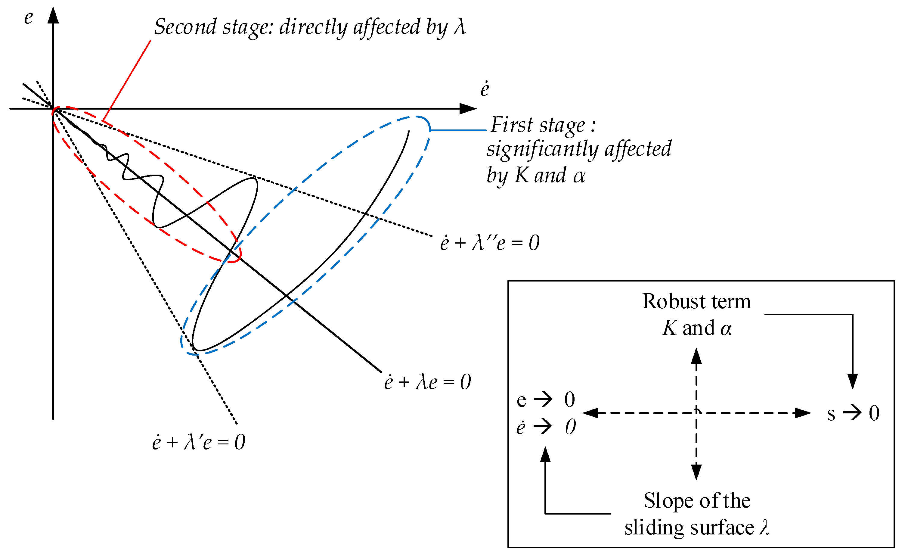
3.3. The Constraint of the Updating Law

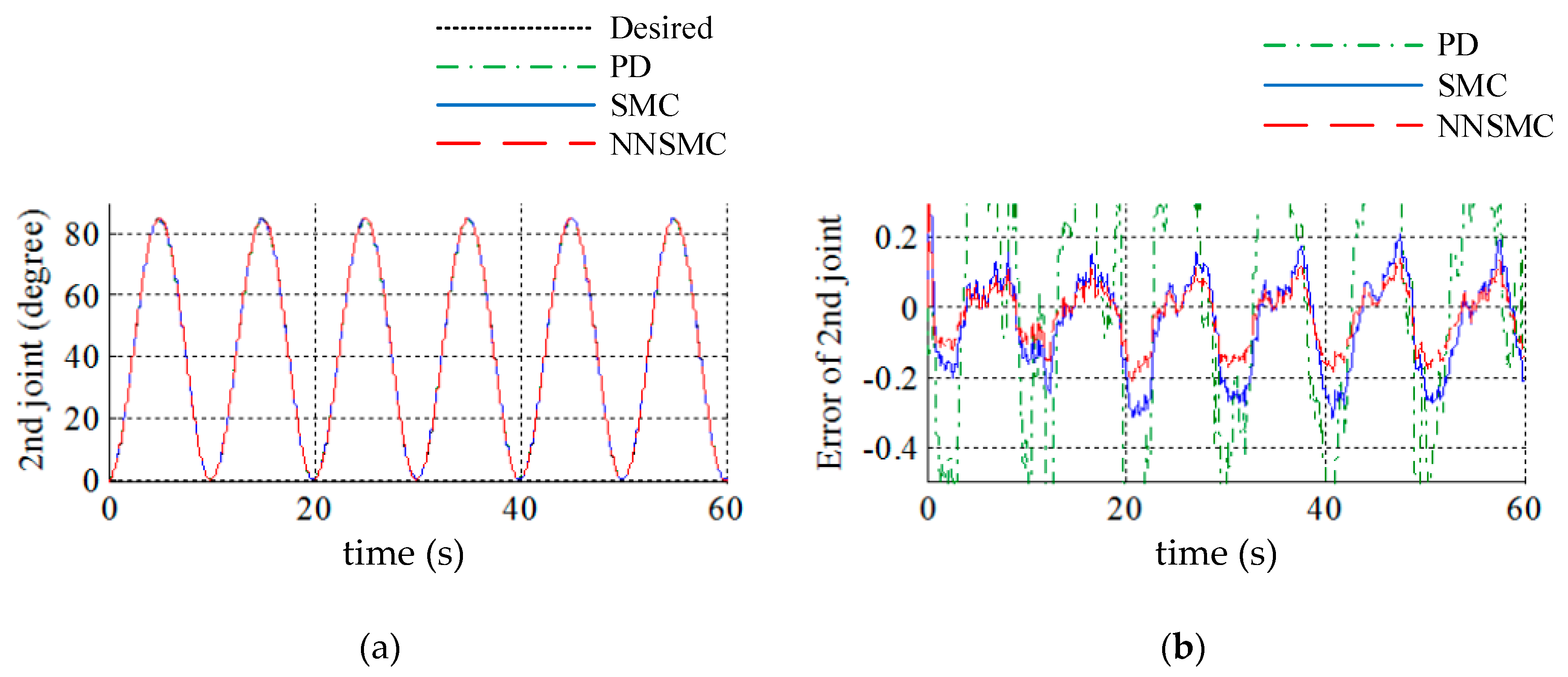
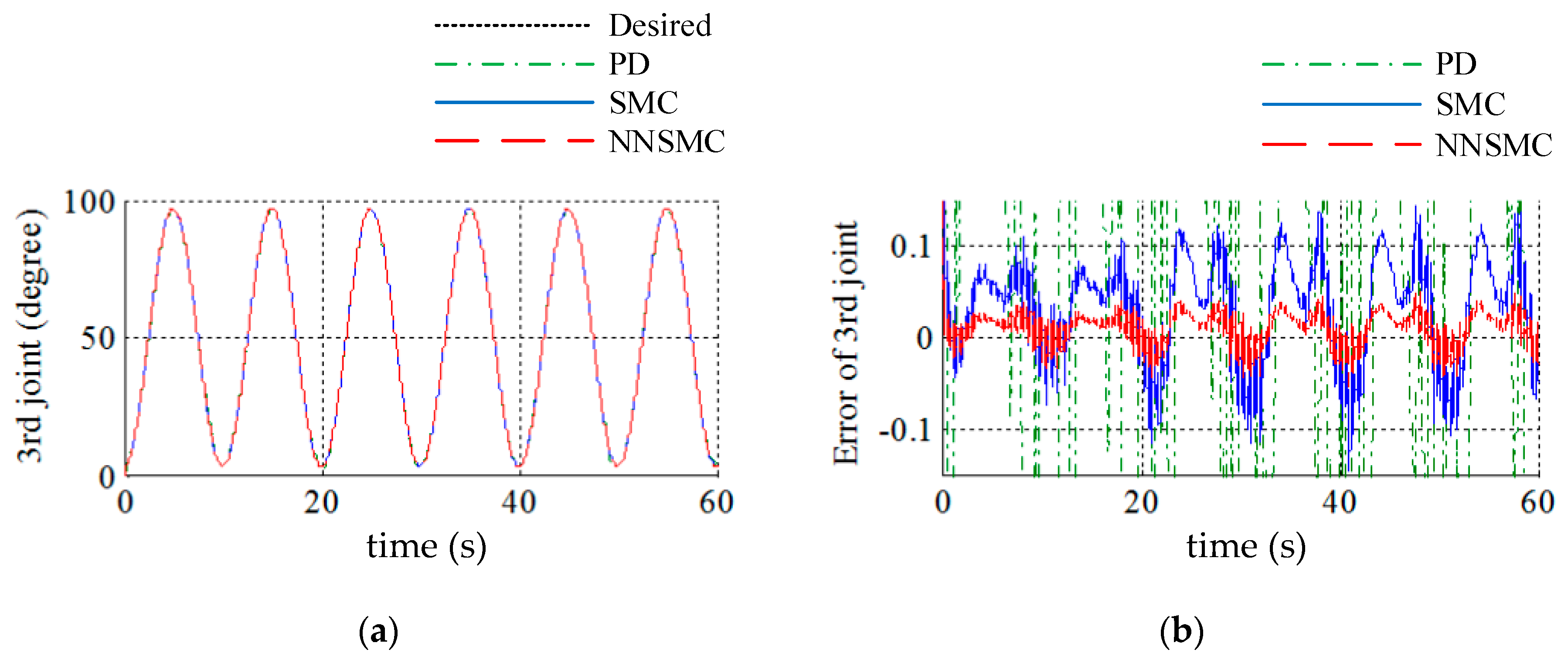
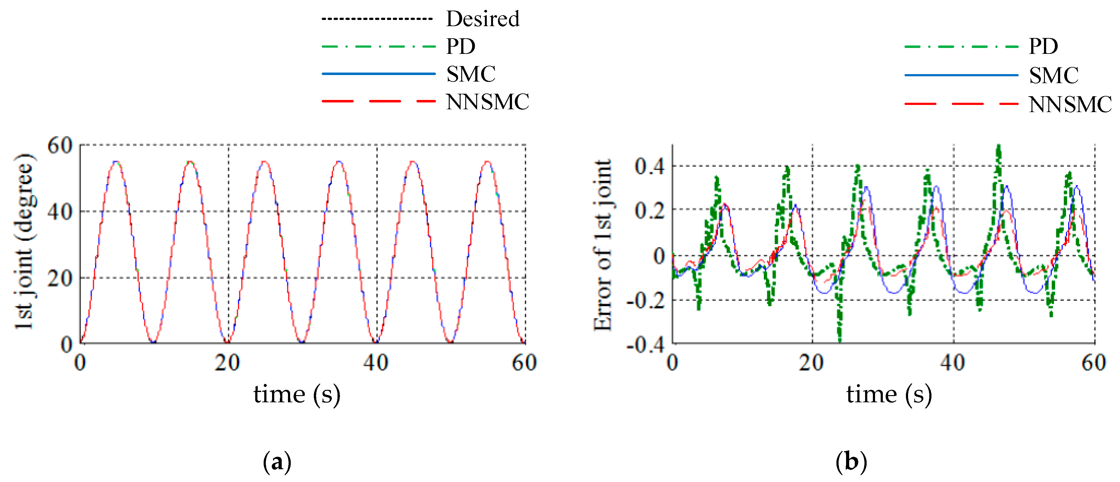
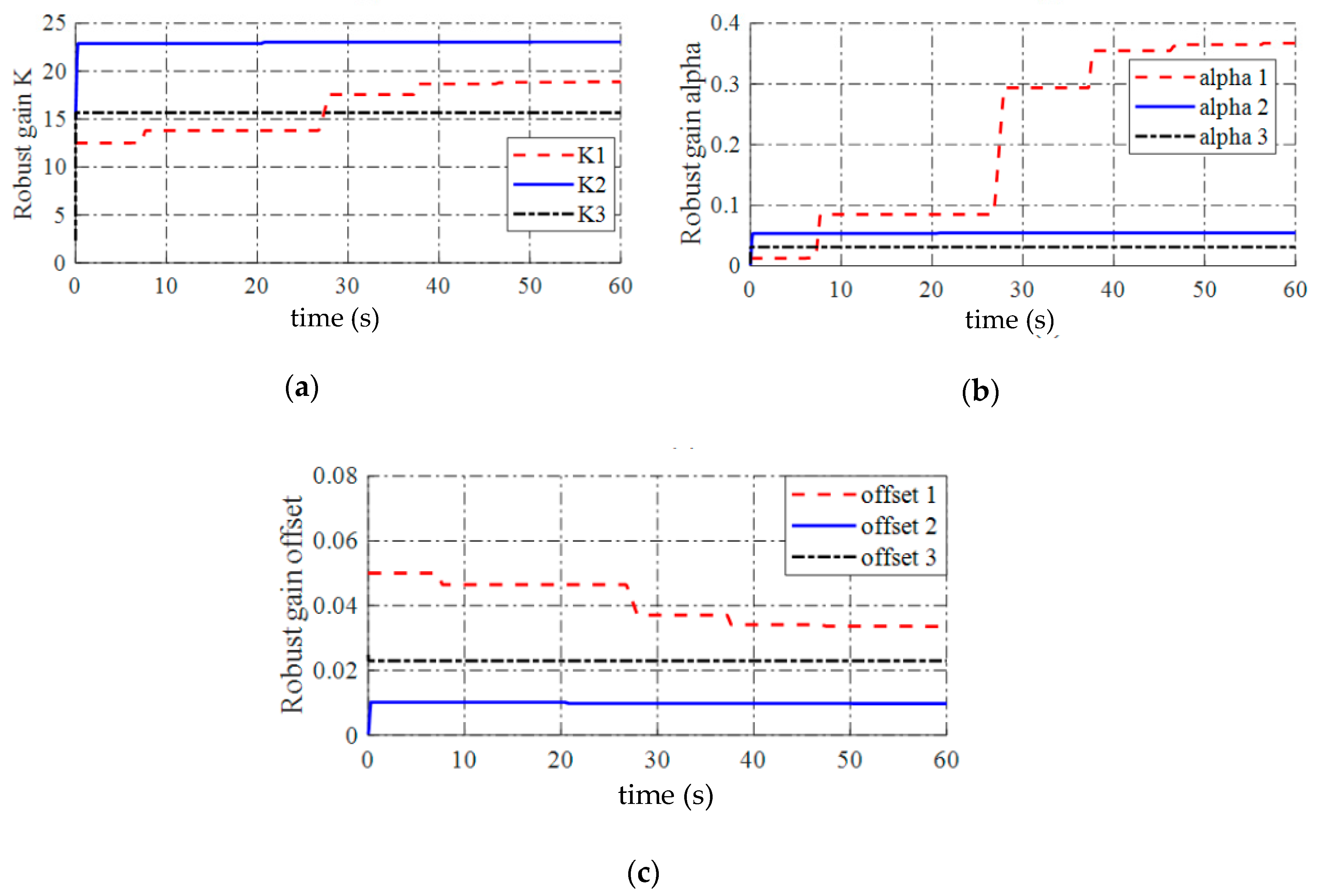
According to Equation (19), the sliding surface is:

$$s_i={\lambda }_{i1}{e}_i+{\lambda }_{i2}{\dot{e}}_i.$$

(40)

When the state trajectory moves towards the sliding surface:

$$s_i={\lambda }_{i1}{e}_i+{\lambda }_{i2}{\dot{e}}_i=0\to {\dot{e}}_i=-\frac{{\lambda }_{i1}}{{\lambda }_{i2}}{e}_i=-{\lambda }_{i-eqv}{e}_i$$

(41)

where ${\lambda }_{i-eqv}=\frac{{\lambda }_{i1}}{{\lambda }_{i2}}$ is an equivalent slope of the sliding surface.

Taking derivative Equation (41) respects to time, we obtain:

$${\displaystyle \underset{0}{\overset{t}{\int }}\frac{{\dot{e}}_i}{e_i}d\phi }=-{\lambda }_{i-eqv}{\displaystyle \underset{0}{\overset{t}{\int }}d\phi }\to e_i=e^{-{\lambda }_{i-eqv}t+C_i}.$$

(42)

Hence, to reduce the convergence time, the updating law for the slope of the sliding surface is then adjusted such that the equivalent slope increases and achieves optimal value:

$${\lambda }_{i-eqv}=\frac{{\lambda }_{i1}}{{\lambda }_{i2}}\to {\lambda }_{i-opt}=\mathrm{constant}.$$

(43)

4. Simulation

Remark 1.

The control signals (voltage) generated from the controller designed are proportional to torques applied on each joint of the manipulator regarding the characteristics of the drivers.

Remark 2.

The initial parameters are chosen based on trial and error such that the highest performance can be achieved. In this study, the learning rate${\eta }_{k_{ij}}$for updating each parameter is designed based on experiments.

Remark 3.

In the simulations, the initial values of the NNSMC are set to be the same as the conventional SMC.

In this section, some simulations were conducted on the MATLAB-Simulink for the 3-DOF manipulator presented in Figure 1. The simulations were carried out with two case studies and comparisons between the proposed algorithm with the conventional controller are discussed to verify the effectiveness in tracking performance. The system parameters are described in

Table 1. The system parameters of the manipulator.

Parameters	Value	Unit
Mass of link	mi (i = 1,2,3) = 5	kg
Length of link 1	l1 = 0.1	m
Length of link 2	l2 = 0.5	m
Length of link 3	l3 = 0.2	m
	d0 = 0.2453	m
	d1 = 0.2471	m
	d2 = 0.036	m

. The estimated inertia, Coriolis, and gravity matrix describing the manipulator dynamics are shown in the Appendix A. The payload profile is described in Figure 5. We considered the payload change to verify the effectiveness of the proposed algorithm.

The initial parameters of the three controllers are shown in

Table 2. Initial parameters of the three controllers.

Controller	Parameter	Value
PD 1 control	Kp	diag (100, 50, 50)
	Kd	diag (10, 10, 10)
SMC 2	λ	diag (10, 10, 20)
	K	diag (12.5, 15, 12.5)
	α	diag (0.005, 0.005, 0.005)
NNSMC 3	λ1	diag (10, 10, 20)
	λ2	diag (1, 1, 1)
	K	diag (12.5, 15, 12.5)
	α	diag (0.005, 0.005, 0.005)
	Ko	diag (0.001, 0.001, 0.001)
Disturbance	f1	diag (0.002, 0.02, 0.02)
	f2	diag (0.002, 0.02, 0.02)

¹ Proportional Derivative control. ² Sliding Mode control. ³ Neural network sliding mode control.

. The reference trajectory of the three joints was designed as:

$$\{\begin{array}{ll}{q}_{1d}=\raisebox{1ex}{$55$}\!\left/ \!\raisebox{-1ex}{$2$}\right.+\raisebox{1ex}{$55$}\!\left/ \!\raisebox{-1ex}{$2$}\right.\sin \left(\raisebox{1ex}{$2\pi t$}\!\left/ \!\raisebox{-1ex}{$10$}\right.-\raisebox{1ex}{$\pi $}\!\left/ \!\raisebox{-1ex}{$2$}\right.\right)& (\mathrm{degree})\\ q_{2d}=\raisebox{1ex}{$85$}\!\left/ \!\raisebox{-1ex}{$2$}\right.+\raisebox{1ex}{$85$}\!\left/ \!\raisebox{-1ex}{$2$}\right.\sin \left(\raisebox{1ex}{$2\pi t$}\!\left/ \!\raisebox{-1ex}{$10$}\right.-\raisebox{1ex}{$\pi $}\!\left/ \!\raisebox{-1ex}{$2$}\right.\right)& (\mathrm{degree})\\ q_{3d}=50+47\sin \left(\raisebox{1ex}{$2\pi t$}\!\left/ \!\raisebox{-1ex}{$10$}\right.-\raisebox{1ex}{$\pi $}\!\left/ \!\raisebox{-1ex}{$2$}\right.\right)& (\mathrm{degree})\end{array}.$$

(44)

The tracking performances of the three joints are depicted in Figure 6, Figure 7, and Figure 8, respectively. The updating of each controller gains of the proposed NNSMC corresponding to three joints are expressed in Figure 9, and the slope of the sliding surfaces is depicted in Figure 10.

As can be seen in Figure 6, Figure 7 and Figure 8, with respect to the response of the three joints, when the external payload increased suddenly at the 20^th second time period, the tracking performance did not change so much, its tracking error when applying the proposed NNSMC was the smallest in comparison with that of PD and conventional SMC, and the stability of the system was maintained. The behavior of the system was adapted by the changing of the controller feedback gains shown in Figure 9 and Figure 10. At the beginning, the initial was set as the same value as the conventional SMC (for the robust gains K and α) and the same as PD (for the ratio between error and the change of error). Regarding the updating law, the controller gains were adjusted in order to achieve a suitable value for the working conditions, thus reducing the tracking error with external payload impacts. The controller gains are described in Figure 9, whereas Figure 10 shows the adjusted slope of the sliding surfaces. Due to the errors in the second and third joints satisfying the constraints, the robust gains of these joints did not change much even when the external payload was attached at the time 20^th second However, due to the structure, the mass inertia of the first joint increased significantly, thus resulting in the time for the first joint to adapt to the change being longer. As opposed to previous works, where only the term $-\alpha \tanh (s)-Ks$ was adjusted to adapt with the working operation, in this study, we considered the slope of the sliding surface as an important parameter that needed to be tuned to minimize the state error. Therefore, the slope of the NNSMC was adjusted depending on the error between the desired and the simulated trajectory to determine the suitable value. When the state trajectory was driven and moved along the sliding surface, the behavior of ${\lambda }_e\hspace{0.17em}$ and ${\lambda }_{de}$ only depended on the state error and its change rate $\dot{e}$. Consequently, the value of ${\lambda }_e$ and ${\lambda }_{de}$ converged and remained at the value in which the steady state was achieved.

5. Experiment

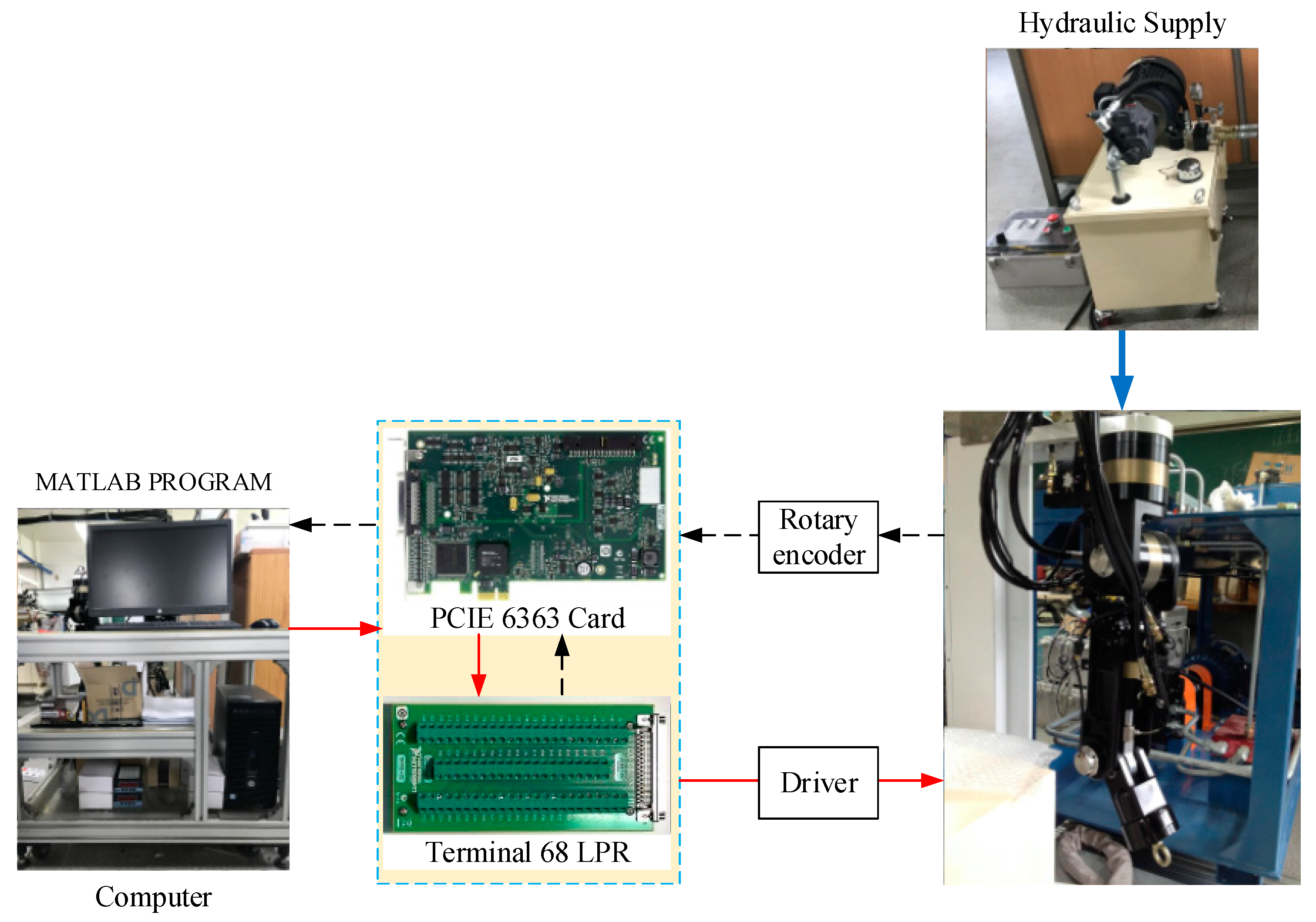
5.1. Experimental Setup

The hardware architecture included a computer (PC) for data processing, a hydraulic supply for the manipulator, and a 3-DOF hydraulic manipulator communicating with the PC via terminal 68 LPR and a PCIE Card (PCIE-6363). The hydraulic manipulator supplied by the hydraulic system was driven by electro-hydraulic actuators equipped with incremental rotary encoders E40H6-5000-3-V-5 to measure the movement. The data read from encoders (incremental) was then processed by the MATLAB program via PCIE card. After processing, the command signal from the computer was sent to the system to force the manipulator to follow the desired trajectory via servo valve amplifier SVA-R-1. The hardware connection is depicted in Figure 11. The dash lines stand for the data obtained from the system, and the solid lines stand for the command signal from the computer.

Remark 4.

In our experiments, the learning rate of each element was set up at a constant value. This value was determined by a trial and error method. Besides, due to the modeling error, the learning rates were scaled in comparison with the simulation.

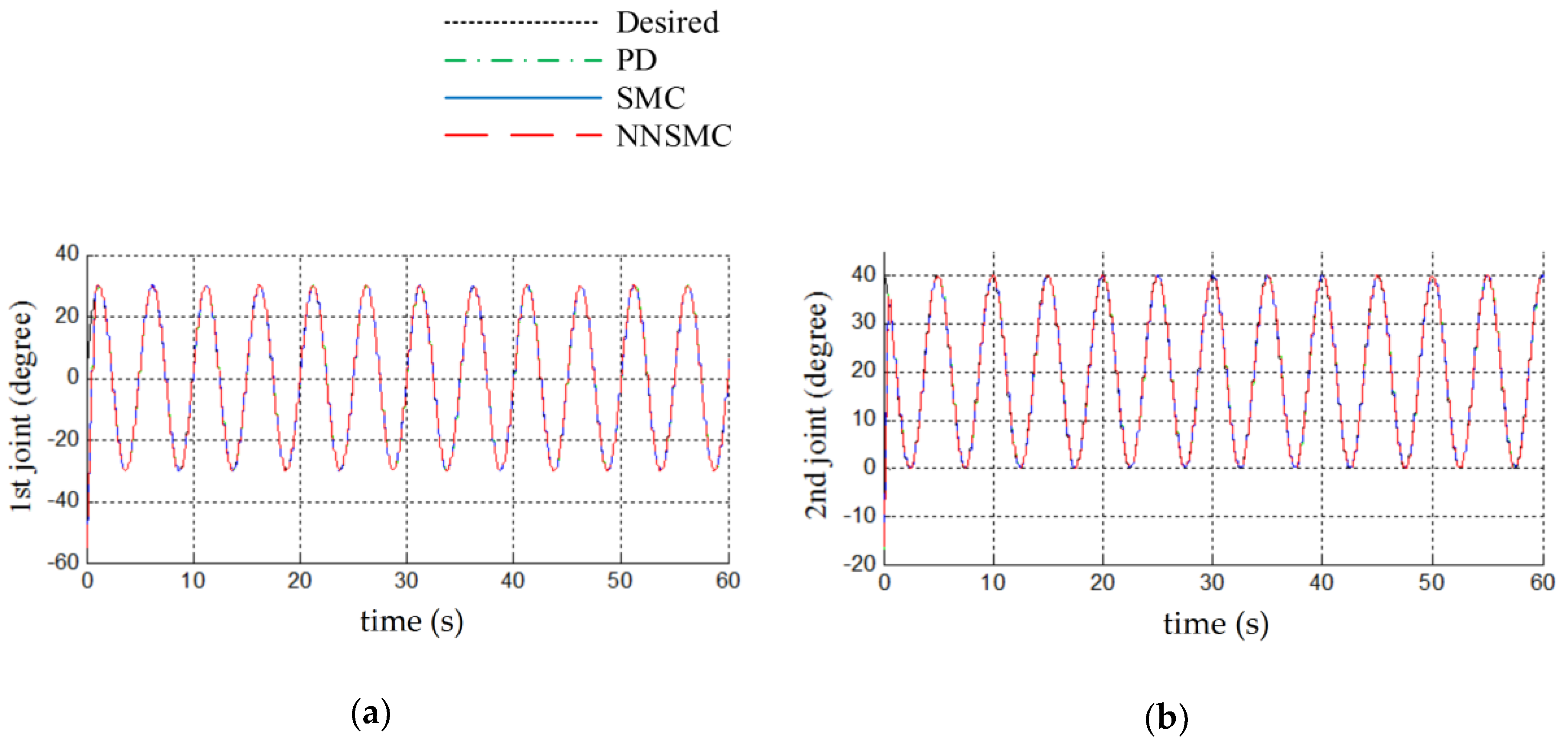
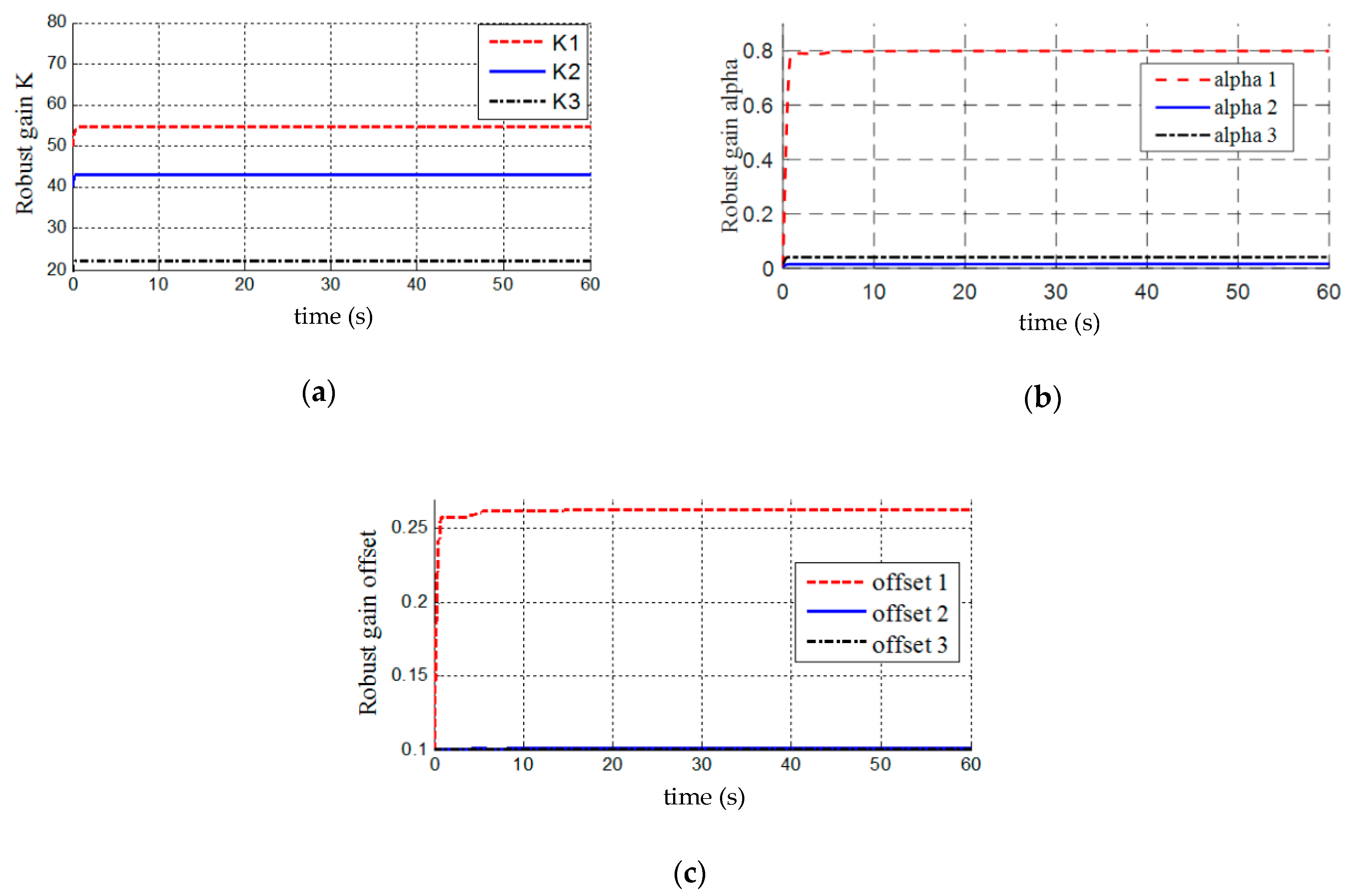
5.2. Experimental Results

In the experiments, the 3-DOF hydraulic manipulator was used to verify the proposed algorithm. The system parameters were supposed to be well known and are presented in Table 1. The desired trajectory is described by the dot-line. The dash-dot line, the solid line, and the dash-line represent the tracking performances of the PD controller, SMC controller, and the NNSMC controller, respectively. The parameters of the PD and SMC controller were manually set and fine-tuned such that the best performance could be achieved, whereas the parameters of the NNSMC are initialized with small values to verify their adaptability. The desired trajectory was designed as:

$$\{\begin{array}{ll}{q}_{1d}=30\sin \left(\raisebox{1ex}{$2\pi t$}\!\left/ \!\raisebox{-1ex}{$5$}\right.\right)& (\mathrm{degree})\\ q_{2d}=20+20\sin \left(\raisebox{1ex}{$2\pi t$}\!\left/ \!\raisebox{-1ex}{$5$}\right.+\raisebox{1ex}{$\pi $}\!\left/ \!\raisebox{-1ex}{$2$}\right.\right)& (\mathrm{degree})\\ q_{3d}=40+20\sin \left(\raisebox{1ex}{$2\pi t$}\!\left/ \!\raisebox{-1ex}{$5$}\right.\right)& (\mathrm{degree})\end{array}.$$

(45)

The comparison in tracking performance and its error of the proposed algorithm with the conventional controllers are depicted in Figure 12 and Figure 13, respectively. The frequency was set at 0.2 Hz to verify the workability of the proposed algorithm. As can be seen in Figure 13, as with the simulation results, the tracking error from the NNSMC was the smallest. However, the slope of the sliding surface of each element reached larger values compared with the simulations due to existing modeling errors inside the actuators. In addition, as opposed to the conventional SMC, the control signals of the NNSMC were modified by adding an offset term K_o to compensate the variations or uncertainties of the system. However, this parameter could not be set to a large value and its learning rate had to be kept at a small value because the large value could affect and degrade the performance of the system.

Compared to the simulation results, the robust gains depicted in Figure 14 changed very quickly at the beginning and tended to be a large value due to the uncertainties. The slope of the sliding surface was changed by tuning the weighting of the two variables e and $\dot{e}$. The first value of the state trajectory could be anywhere depending on the initial value of the system. Then adjusting the slope of the sliding surface at the same time with tuning robust term could drive the system error convergence to zero (ideal case) or a boundary quickly. The adaptive slopes of the three joints are presented in Figure 15. The profiles of the adjusted parameters in the experiment result were quite similar to the simulation due to uncertainties or disturbance existing in the real mechanical structure.

6. Conclusions

This paper presented the neural network based sliding mode control for tracking control of the 3-DOF manipulator with the presence of uncertainties and external payload variation. The structure of the neural network sliding mode control as well as the correlation between the slope of the sliding surface and robust term in the control signal are derived. The conventional sliding mode controller (SMC) is described by nonlinear terms, the sliding surface and the robust term with gain K, and α via the term “–Ks– αsign(s)” to generate the tracking performance. As mentioned in the introduction and in Section 3.2, despite its strong robustness, fixed gains cannot satisfy the tracking performance with the variant uncertainties or external disturbances. Previous works proposed many control schemes for the SMC with adaptive gains by using intelligent techniques without considering the slope of the sliding surface that affects the convergence rate to zero of the system errors. Besides, suitable gains are not discussed clearly. Based on a missing in constructing an advanced algorithm on constructing an advanced algorithm, this paper employed the neural network with gradient descent method for adjusting the robust term and the slope of the sliding surface (same function as nonlinear PD control) to a suitable value such that the stability is guaranteed, and higher tracking performance can be achieved. The proposed controller is tested on the 3 DOF hydraulic manipulator to validate its effectiveness and workability. Comparisons of tracking performance between the proposed algorithm with the conventional sliding mode and traditional PD control are given in both simulation and experiments under the presence of the uncertainties and the external payload. The results indicate that the proposed algorithm can exhibit high precision in tracking performance.

However, in this study, the learning rate parameters are set manually based on several experiments as mentioned in the above remarks. These parameters should be automatically adopted with system behavior. Besides, we ignored use of the intelligent technique as compensation like other convention adaptive sliding mode controller schemes. Therefore, the neural network SMC proposed in this study is a premise to develop an adaptive learning rate and can be considered as the first step to get a suitable value for a novel adaptive control with intelligent techniques (radial basis function or adaptive control) in future works.

References

1. John, J.C. Introduction to Robotics Mechanics and Control, 3rd ed.; Addison-Wisley: Reading, MA, USA; Pearson Education Inc.: Upper Saddle River, NJ, USA, 1989. [Google Scholar]
2. Yuxin, S.; Peter, C.M.; Chunhong, Z. Global Asymptotic Saturated PID Control for Robot Manipulators. IEEE Trans. Control Syst. Technol. 2010, 18, 1280–1288. [Google Scholar]
3. Woosoon, Y.; Sahjendra, N.S. Feedback Linearization of Differential-Algebraic Systems and Force and Position Control of Manipulators. In Proceedings of the 1993 American Control Conference, San Francisco, CA, USA, 2–4 June 1993; pp. 2279–2283. [Google Scholar]
4. Chaouki, A.; Darren, M.D.; Peter, D.; Mohammad, J. Survey of the robust control robots. IEEE Control Syst. Mag. 1991, 12, 24–30. [Google Scholar]
5. Ishii, C.; Shen, T.; Tamura, K. Robust model-following control for a robot manipulator. IEEE Proc. Control Theory Appl. 1997, 144, 53–60. [Google Scholar] [CrossRef]
6. Frank, L.L.; Aydin, Y.; Kai, L. Multilayer neural-net robot controller with guaranteed tracking performance. IEEE Trans. Neural Netw. 1996, 7, 388–399. [Google Scholar]
7. Shuzhi, Z.G.; Christopher, J.H. Adaptive Neural Network Control of Robotic Manipulator; World Scientific Publishing Co., Inc.: River Edge, NJ, USA, 1998. [Google Scholar]
8. Ha, T.W.; Jun, K.H.; Nguyen, M.T.; Han, S.M.; Shin, J.W.; Ahn, K.K. Position control of an Electro-Hydrostatic Rotary Actuator using adaptive PID control. J. Drive Control 2017, 14, 37–44. [Google Scholar]
9. Rong, J.W.; Rajkumar, M. Design of Fuzzy-Neural-Network-Inherited Backstepping Control for Robot Manipulator Including Actuator Dynamics. IEEE Trans. Fuzzy Syst. 2014, 22, 709–722. [Google Scholar]
10. Nikdel, N.; Badamchizadeh, M.A.; Azimirad, V.; Nazari, M.A. Adaptive backstepping control for an n-degree of freedom robotic manipulator based on combined state augmentation. Robot. Comput. Integr. Manuf. 2017, 44, 129–143. [Google Scholar] [CrossRef]
11. Li, S.; Ahmad, G.; Xie, W.; Gao, Y. An Enhanced IBVS Controller of a 6DOF Manipulator Using Hybrid PDSMC Method. Int. J. Control Autom. Syst. 2018, 16, 844–855. [Google Scholar] [CrossRef]
12. Shafiqul, I.; Xiaoping, P.L. Robust Sliding Mode Control for Robot Manipulators. IEEE Trans. Ind. Electron. 2011, 58, 2444–2453. [Google Scholar]
13. Illias, E.M.; Carlos, R.G.; Dirk, L.; Bram, V. The Variable Boundary Layer Sliding Mode Control: A Safe and Performant Control for Compliant Joint Manipulators. IEEE Trans. Robot. Autom. Lett. 2017, 2, 187–192. [Google Scholar]
14. Lee, H.S.; Won, S.J.; Ahn, K.K. The Numerical Modeling and Sliding Mode Control of a New Submersible Fish Cage. J. Drive Control 2017, 14, 18–24. [Google Scholar]
15. Jaemin, B.; Jin, M.; Han, S.H. A New Adaptive Sliding-Mode Control Scheme for Application to Robot Manipulators. IEEE Trans. Ind. Electron. 2016, 63, 3628–3637. [Google Scholar]
16. Ahmed, F.A.; Elsayed, A.S.; Wael, M.E. Adaptive fuzzy sliding mode control using supervisory fuzzy control for 3 DOF planar robot manipulators. Appl. Soft Comput. 2011, 11, 4943–4953. [Google Scholar]
17. He, J.; Luo, M.; Zhang, Q.; Zhao, J.; Xu, L. Adaptive Fuzzy Sliding Mode Controller with Nonlinear Observer for Redundant Manipulators Handling Varying External Force. J. Bionic Eng. 2016, 13, 600–611. [Google Scholar] [CrossRef]
18. Do, H.T.; Hyung, G.P.; Kyoung, K.A. Application of an adaptive fuzzy sliding mode controller in velocity control of a secondary controlled hydrostatic transmission system. Mechatronics 2014, 24, 1157–1165. [Google Scholar] [CrossRef]
19. Nguyen, S.D.; Choi, S.B.; Seo, T.I. Adaptive Fuzzy Sliding Control Enhanced by Compensation for Explicitly Unidentified Aspects. Int. J. Control Autom. Syst. 2017, 15, 2906–2920. [Google Scholar] [CrossRef]
20. Do, H.T.; Dang, T.D.; Truong, H.V.A.; Ahn, K.K. Maximum Power Point Tracking and Output Power Control on Pressure Coupling Wind Energy Conversion System. IEEE Trans. Ind. Electron. 2018, 65, 1316–1324. [Google Scholar] [CrossRef]
21. Tu, D.C.T.; Kyounbg, K.A. Nonlinear PID control to improve the control performance of 2 axes pneumatic artificial muscle manipulator using neural network. Mechatronics 2006, 16, 577–587. [Google Scholar]
22. Sun, T.; Pei, H.; Pan, Y.; Zhou, H.; Zhang, C. Neural network-based sliding mode adaptive control for robot manipulators. Neurocomputing 2011, 74, 2377–2384. [Google Scholar] [CrossRef]
23. Tran, M.D.; Hee, J.K. Adaptive terminal sliding mode control of uncertain robotic manipulators based on local approximation of a dynamics system. Neurocomputing 2017, 228, 231–240. [Google Scholar] [CrossRef]
24. Seul, J. Stability Analysis of Reference Compensation Technique for Controlling Robot Manipulators by Neural Network. Int. J. Control Autom. Syst. 2017, 15, 952–958. [Google Scholar]
25. Seul, J. Improvement of Tracking Control of a Sliding Mode Controller for Robot Manipulators by a Neural Network. Int. J. Control, Autom. Syst. 2018, 16, 937–943. [Google Scholar]
26. Vo, A.T.; Kang, H.-J. An Adaptive Neural Non-Singular Fast-Terminal Sliding-Mode Control for Industrial Robotic Manipulators. Appl. Sci. 2018, 8, 2562. [Google Scholar] [CrossRef]
27. To, X.D.; Ahn, K.K. Radial Basis Function Neural Network based Adaptive Fast Nonsingular Terminal Sliding Mode Controller for Piezo Positioning Stage. Int. J. Control Autom. Syst. 2017, 15, 2892–2905. [Google Scholar]
28. Vu, T.Y.; Wang, Y.N.; Pham, V.C.; Nguyen, X.Q.; Vu, H.T. Robust Adaptive Sliding Mode Control for Industrial Robot Manipulator Using Fuzzy Wavelet Neural Networks. Int. J. Control Autom. Syst. 2017, 15, 2930–2941. [Google Scholar]
29. Ahn, K.K.; Huynh, T.C.N. Intelligent switching control of a pneumatic muscle robot arm using learning vector quantization neural network. Mechatronics 2007, 17, 255–262. [Google Scholar] [CrossRef]
30. Saeed, P.; Sajad, B.; Ali, J. Performance Analysis of a Neuro-PID Controller Applied to a Robot Manipulator. Int. J. Adv. Robot. Syst. 2012, 9, 163. [Google Scholar]
31. Le, T.D.; Kang, H.-J.; Suh, Y.-S.; Ro, Y.-S. An online self-gain tuning method using neural networks for nonlinear PD computed torque controller of a 2-dof parallel manipulator. Neurocomputing 2013, 116, 53–61. [Google Scholar] [CrossRef]
32. Yuri, S.; Christopher, E.; Leonid, F.; Arie, L. Sliding Mode Control and Observation, Control Engineering; Springer: New York, NY, USA, 2014. [Google Scholar]
33. Wilfrid, P. Sliding Mode Control in Engineering; Marcel Dekker, Inc.: New York, NY, USA, 2002. [Google Scholar]
Figure 1. An overview of the 3-degrees of freedom (DOF) hydraulic manipulator: (a) 3D drawing; (b) principle drawing.
Applsci 09 02023 g001
Figure 2. The architecture of the last link.
Applsci 09 02023 g002
Figure 3. The motion of the state trajectory of the sliding mode control in which the two stages and the two terms affecting the convergence rate of the state error are considered. The sub-figure shows the correlation between the robust term K and α with the slope of the sliding surface λ.
Applsci 09 02023 g003
Figure 4. An architecture of the proposed neural network based sliding mode control.
Applsci 09 02023 g004
Figure 5. The external payload mass profile.
Applsci 09 02023 g005
Figure 6. Comparison of tracking performance of the first joint: (a) tracking position, (b) tracking error.
Applsci 09 02023 g006
Figure 7. Comparison of tracking performance of the second joint: (a) tracking position, (b) tracking error.
Applsci 09 02023 g007
Figure 8. Comparison of tracking performance of the third joint: (a) tracking position, (b) tracking error.
Applsci 09 02023 g008
Figure 9. The adaptive gains: (a) Robust gain K, (b) α, (c) offset gains of ith joint, where i = 1,2,3 with respect to the first joint, the second joint, and the third joint.
Applsci 09 02023 g009
Figure 10. The slope adjusted for the sliding surface of the (a) first joint, (b) second joint, (c) third joint.
Applsci 09 02023 g010
Figure 11. The hardware setup for the 3-DOF manipulator.
Applsci 09 02023 g011
Figure 12. Comparison of the tracking performance of the three joints: (a) first joint, (b) second joint, (c) third joint.
Applsci 09 02023 g012aApplsci 09 02023 g012b
Figure 13. Comparison of the tracking error of the three joints: (a) first joint, (b) second joint, (c) third joint.
Applsci 09 02023 g013
Figure 14. The adaptive gains: (a) Robust gain K, (b) α, (c) offset gains of the ith joint, where i = 1,2,3 with respect to the first joint, the second joint, and the third joint.
Applsci 09 02023 g014
Figure 15. The slope adjusted for the sliding surface of the (a) first joint, (b) second joint, (c) third joint.
Applsci 09 02023 g015