Low-Frequency Magnetic Scanning Device and Algorithm for Determining the Magnetic and Non-Magnetic Fractions of Moving Metallurgical Raw Materials

Abstract

The development of an algorithm to automate the process of measuring the magnetic properties of macroscopic objects in motion is an important problem in various industries, especially in ferrous metallurgy and at factories where ferrous scrap is a strategic raw material. The parameter that requires work control is the hidden mass fraction of a non-magnetic substance that is present in the ferromagnetic raw material. The solution to this problem has no prototypes. In our work, a simple measuring device and a mathematical algorithm for calculating the mass fraction of the non-magnetic fraction in a strongly magnetic matrix were developed. The device is an inductance coil, in which the angle of the electromagnet losses is related to the mass of the magnetic material moving the coil. The magnitude of the instantaneous values of the lost angle integral was compared with the result of weighing the object on scales. This allowed us to calculate the proportion of the magnetic and non-magnetic fractions. The use of this prototype is herein illustrated. The experimental results of the determination of the magnetic-fractional composition depending on the mass of scrap metal and its bulk and the magnetic characteristics are presented.

1. Introduction

Physical Background of the Method

Automating the measurement process of the magnetic properties of macro-objects in motion is a task in various industries where ferrous scrap is a common raw material. The capability to directly control the metallic raw material composition in moving transport without unloading and sampling is a scientific and technical problem which is gaining much attention [1,2].

Operation monitoring is mainly required to control the various forms of the hidden mass fraction of non-magnetic substances present in ferromagnetic raw materials. Non-magnetic inclusions add technologically useless weight to the freight, which is documented during weighing and included in the subsequent financial calculations. The damage caused by non-magnetic inclusions in railway freight per annum adds up to more than seven billion rubles of direct financial losses in Russia. At present, there is no system, device, or unit that enables the express control of these inclusions without stopping or unloading the train or automobile. The closest analogues are X-ray television (TV) units, which are being positioned by some developers as instruments for freight truck express control [3,4]. In addition to high technical and maintenance costs, the usage of high-powered sources of ionizing radiation for express control has a series of restrictions related to work safety standards. X-ray measurements are vulnerable to video signal distortion via special freight stowing and X-ray radiation shielding. X-ray measurements offer no ability to evaluate the non-magnetic material mass fraction.

Various metal detectors [3,4,5,6] offer no solution to the problem of non-magnetic substance quantity control in ferrous material, since a metal detector’s purpose is to reveal insignificant quantities of metal in non-magnetic or weakly magnetic media, which is an inverse problem to the one considered here.

Numerous works on magnetic induction tomography [7,8,9,10,11] were devoted to magnetic scanning of biological objects, which solves the same problem as the metal detectors—measuring a weak magnetic signal in a non-magnetic medium. However, the difference in magnetic induction tomography compared to metal detectors is that it uses mathematical signal processing, for example, a three-dimensional (3D) finite-element method (FEM) [12,13,14]. Therefore, tomography can produce a 3D picture of the distribution of magnetic centers by scanned volume. Mathematically, this is achieved by the region being divided into a finite number of subdomains (elements), where the solutions of differential equations are sought. In each of the elements, the type of the approximating function is chosen arbitrarily. The coefficients of the approximating functions are usually sought from the condition of the equality of the value of neighboring functions at the boundaries between the elements (at the nodes). These coefficients are then calculated for the functions of the elements in the nodes. A system of linear algebraic equations is compiled and solved. However, this method is not applicable to the task of searching for a signal of non-magnetic inclusions in a ferromagnetic medium at low frequencies. The task of detecting weakly magnetic signals in a non-magnetic matrix is solved using high frequencies to scan an object (at hundreds and thousands of megahertz [7]). This approach is fundamentally not applicable to solving our inverse problem of searching for non-magnetic inclusions in a strongly magnetic matrix. Scanning a ferromagnetic material with a high-frequency field will lead to a strong decrease in the amplitude of the electromagnetic waves as they penetrate deep into the conducting medium [15]. As a result of this effect, a high-frequency alternating current, when flowing through a conductor, is distributed mainly in the surface layer. This shields the signals from the depths of the object. In our case, a railway car will screen the signal from the load. The use of low frequencies (several tens of hertz) for scanning moving magnetic objects does not allow for the use of the FEM, since the wavelength for low sound frequencies is about 10 m. This limits the minimum size of the object being examined. Additionally, this leads to a few areas, each with a very large size, being partitioned, which does not allow for compiling of the correct system of equations. Therefore, to date, we are not aware of any attempts to create low-frequency magnetic scanning devices that can be used for large-sized ferromagnetic objects with a high magnetic signal. Thus, for the first time, in this work we propose a new device and a new algorithm for processing a low-frequency electromagnetic signal from an object, which mainly consists of a magnetic fraction, with the addition of non-magnetic inclusions. The principle of scanning such an object is to consistently measure the magnetic signal and to measure the total mass of the object. Non-magnetic inclusions do not contribute to the magnetic component of the signal, but they contribute to the total mass of the object. In some cases, this allows us to estimate the mass fractions of the magnetic and non-magnetic fractions. The best method for measuring a low-frequency magnetic signal is a conventional high-inductance solenoid (inductance coil). The express control process, which is based on the measurement of the parameters of the inductor coil, through which the inspected freight passes at its core, is free from the aforementioned drawbacks. The dimensions of the solenoid compared to the length of the object being measured, with an approximation sufficient for our purposes, enable application of the equations describing the inductance of a long solenoid (Figure 1).

Solenoid coil inductance can be calculated with the following equation [15]:

$$L=A_L{\mu }_r{N}^2$$

(1)

where $N$ is the turn number of the coil, ${\mu }_r$ is the relative magnetic permeability of the coil core (when there is a core), and $A_L$ is the coefficient defined by the coil geometric parameters:

$$A_L={\mu }_0\frac{S_e}{l_e},$$

(2)

where μ₀ is the vacuum magnetic permeability, S_e is the cross-section area of the coil (core), and $l_e$ is the effective magnetic path length. Equations (1) and (2) show that coil inductance is directly proportional to the core magnetic permeability (susceptibility), and the core cross-section area. Thus, any non-magnetic or weakly magnetic inclusions in the core (freight) will add to the coil inductance to an extent that can be calculated when measuring this parameter (or values related to it) and will connect it with the mass-dimensional characteristics of the inspected freight.

The application of a sinusoidal alternating voltage to the ideal inductance coil, i.e., to the coil with zero ohmic resistance, the zero capacity, and no core, results in the appearance of an alternating current in the coil that changes with time according to sinusoidal law and lags behind the voltage by which it was caused by $\pi /2$. The actual coil with no core is characterized by finite ohmic resistance and capacity, so the circuit equivalent to the coil may be presented as active (ohmic) resistance $R$, connected in a series with inductive resistance $X_L$, both of them connected in parallel to reactive capacitive resistance $R_C$, the two latter values being calculated via the following equations respectively [15]:

$$X_L=\omega L,$$

(3)

$$R_C=\frac{1}{\omega C_k},$$

(4)

where $L$ is the coil inductance, $C_k$ is the coil capacity, ω = 2πf is the cyclic frequency, and $f$ is the alternating voltage (current) frequency.

The presence of active resistance $R$ and reactive capacitive resistance $X_C$ results in an additional (compared to $\pi /2$ in the perfect coil) phase shift ${\phi }_L$ (loss angle), which thus characterizes the energy loss in the coil on $R_{\Omega }$ and $R_C$ resistances [16,17]. The losses in the coil are usually characterized by a loss angle tangent ($tg{\phi }_L$) and its reciprocal value, which is called the quality factor $Q$. When determining the quality factor, all resistances related to losses are combined in the loss resistance $R_L$:

$$Q=\frac{X_L}{R_L}=\frac{1}{tg{\phi }_L},$$

(5)

where, in the case of core presence, $R_L$ can be generally written as

$$R_L=R_{\Omega }+R_C+R_{core}$$

(6)

where $R_{\Omega }$ is the ohmic resistance, $R_C$ is the capacitive resistance, and $R_{core}$ is the resistance corresponding to the losses in a core.

The $R_{\Omega }$ and $R_C$ resistances describe the losses directly in the coil and material of its frame respectively, and the resistance $R_{core}$ corresponds to the losses in the core material.

Losses in a conductor (wire) are described by active (ohmic) resistance, which can be calculated according to the following equation:

$$R_{\Omega 0}=\rho \frac{l}{S}=\frac{4l}{\pi d^2}\rho ,$$

(7)

where $l$ is the length of the wire, $d$ is the diameter of the wire, $\rho$ is the resistivity, and $S$ is the cross-sectional area of the wire. Therefore, the ohmic (active) losses in the conductor can be considered if the parameters of the coil and its windings are known.

The capacitive resistance of the $R_C$ explains the losses in the conductor insulation material and in the coil body. The resistance of $R_{core}$ can be represented as the sum of $R_{ed}$ corresponding to eddy current losses, and $R_M$ corresponding to losses of magnetic nature. $R_{ed}$, eddy currents (Foucault currents), are induced in the core of the material coil by the alternating electromagnetic field generated by the coil. These currents contribute to losses due to their dissipation in the core. $R_M$ corresponds to the loss of the magnetic nature caused by the hysteresis phenomenon. Thus, on the basis of the aforementioned, information about the magnetic state of the coil’s core can be obtained from the inductance of the coil, and it is also possible to separate the characteristics of the coil itself from the characteristics of the material being measured.

Conclusions about the mass, density, and surface area of the magnetic material can be drawn from the measurement of the specified parameters of the car with a load as its core. The morphology of the load, the anisotropy of its characteristics, and its spatial and magnetic orientation can also be determined [15].

If a magnetic measurement to estimate the mass of a magnetic object occurs after measurement on a railway scale, then conclusions on the mass, density, and surface area of the magnetic material can be made from measurements of the indicated parameters of the coil with a load as its core. Non-magnetic materials including earth, concrete, polymers, and others, do not affect the magnetic signal, but significantly change the weight of the car with the load. This pattern underlies the operation of the device. The methods used for determining and accounting for the spatial morphology and magnetic orientation were analyzed in this study and applied in a real-life sample.

2. Materials and Methods

The physical model is described with some simplifications to prevent unauthorized reproduction of intellectual property.

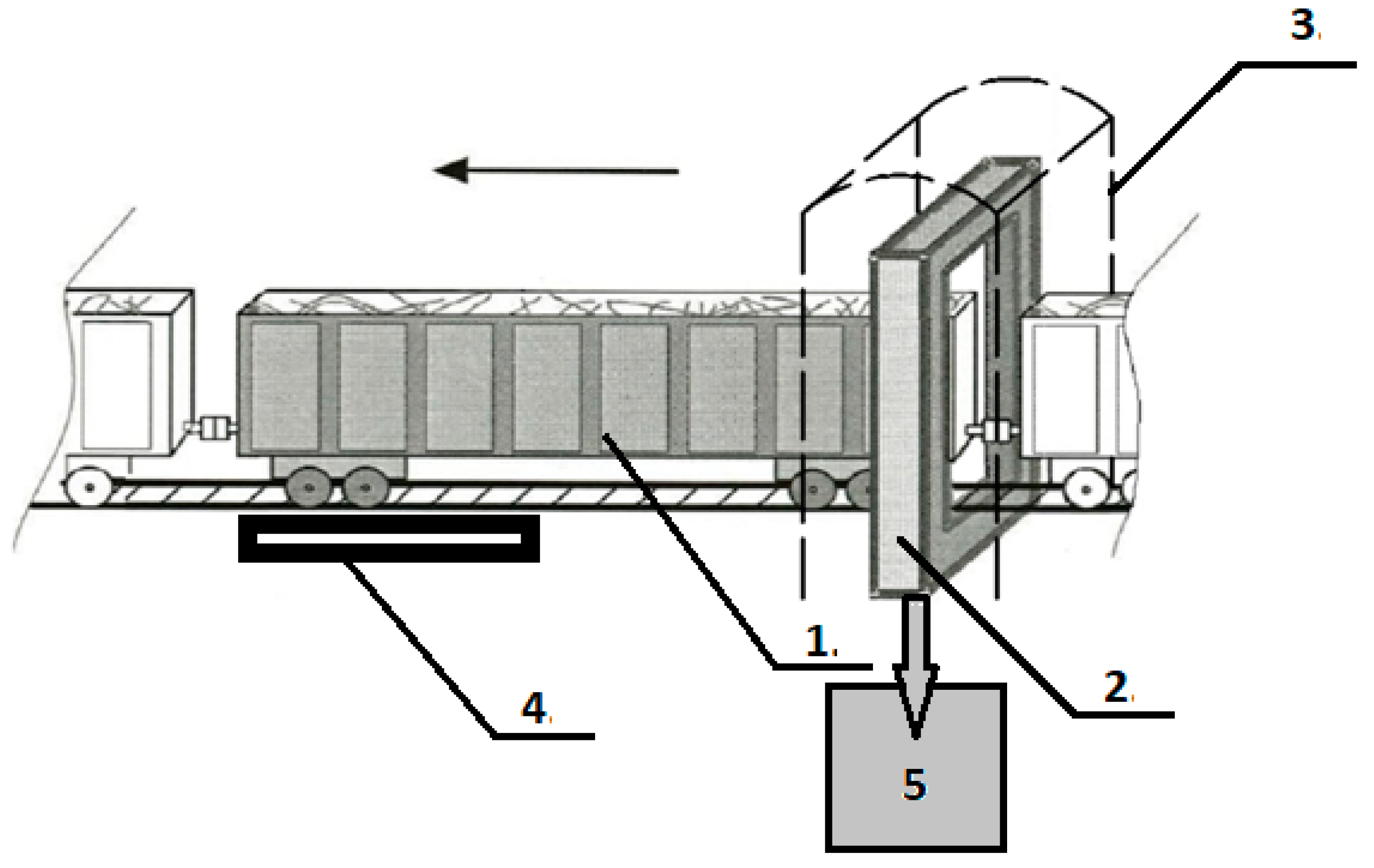
2.1. Experimental Setup and Calculation Principle

The measuring unit is a solenoid coil located around the railway track. The meter contains two windings: generating and measuring. The generating winding creates an alternating electromagnetic field with constant frequency and intensity parameters. The measuring winding induction current is induced with instantaneous parameters depending on the local properties of the moving core of the solenoid. The object being measured serves as the core, which is a moving railway car in our case. The parameters of the measuring device are shown in

Table 1. Parameters of the measuring coil system and electric signals used in measurements.

Parameter Name	Value	Unit
Range of alternating current in primary winding	2.00–8.00 ± 0.05	A
Range of alternating magnetic field strength	100–1000	A/m
Range of alternating current frequency	20–100 ± 1	Hz
Windings real resistance (Ω)
-magnetizing winding	1 ± 0.2	Ω
-measuring winding	12.5 ± 2	Ω
Estimated value of the measuring coil cross-section area	43.43 ± 0.01	m2
Reference value of magnetic flux in air	1.9·10−2	Wb
Range of magnetic flux measurement	1.5 × 10−2–6.0 × 10−2	Wb
Dimensions of measuring coil	7190 × 6040 × 740	mm

.

Figure 1 shows a diagram of the setup that was used to record the measurements. The parameters of the measuring coil system and electric signals used in the measurements are listed in Table 1. The measuring coil system consists of primary and secondary windings.

The inductance of a coil with a solenoid within is calculated using Equations (8) and (9):

$$L=\frac{\mathsf{\Phi }}{I},$$

(8)

$$\mathsf{\Phi }=N{S}_{p}H,$$

(9)

where $L$ is the inductance, $I$ is the current, $\mathsf{\Phi }$ is the magnetic flux, $N$ is the turn number, $S_p$ is the solenoid cross-section area, and $H$ is the magnetic field strength.

If there is no metallic core inside the solenoid frame, inductance is calculated according to Equation (1), with permeability considered as being $I$, which is the permeability of air:

$$L=\frac{N{S}_{p}H}{I},$$

(10)

$$I=\frac{H{l}_{av}}{N},$$

(11)

where $l_{av}$ is the average length of line of the magnetic force.

Therefore, in the case of a coil without a core:

$$L_{air}=\frac{N{S}_{p}H}{I}=\frac{N{S}_{p}H}{H\frac{l_{av}}{N}}=\frac{N^2{S}_{p}H}{H{l}_{av}}=\frac{N^2{S}_p}{l_{av}}$$

(12)

When the ferrous core passes through the coil, additional inductance appears within the coil:

$$L_{met}=\frac{N^2{S}_{met}B}{H{l}_{av}}=\frac{\mu N^2{S}_{met}}{l_{av}},$$

(13)

$$B=\mu H,$$

(14)

where $B$ is the magnetic inductance, $\mu$ is the magnetic permeability, and $S_{met}$ is the cross-section area of the railway carriage with metal. The total inductance is:

$$L_{sum}=L_{air}+L_{met}=\frac{N^2\left(S_p-S_{met}\right)}{l_{av}} +\frac{{\mu }_{\mathrm{MeT}}{N}^2\ast S_{met}}{l_{av}}=\frac{N^2}{l_{av}}\left(S_p-S_{met}+{\mu }_{met}{S}_{met}\right),$$

(15)

where $\mu$ is the magnetic permeability of metal.

With the help of Equation (15), it is possible to calculate the quality factor $Q$:

$$Q=2\pi f\frac{L_{sum}}{R}=tg\Delta \phi ,$$

(16)

$$\Delta \phi ={\phi }_{\mathrm{u}}-{\phi }_{\mathrm{I}},$$

(17)

where ${\phi }_{\mathrm{u}}$ is the voltage phase, ${\phi }_{\mathrm{I}}$ is the current phase, $\Delta \phi$ is the phase difference between current and voltage in the primary winding, and $R$ is the resistance.

Let us determine the loss angle ${\phi }_L$ as

$${\phi }_L={90}^0-\left|\Delta \phi \right|.$$

(18)

Then, rewrite Equation (16) as

$$\frac{R}{tg{\phi }_L}=2\pi fL.$$

(19)

It is possible to write inductance as a function of the mass of metal inside the coil:

$$L=\frac{R}{2\pi ftg{\phi }_L}=\frac{N^2}{l_{av}}\left(S_p-S_{met}+{\mu }_{met}{S}_{met}\right),$$

(20)

$$l_{av}= \frac{m}{\rho S_{met}},$$

(21)

$$m= \frac{2\pi f\rho S_{met}\ast N^2\left(S_p-S_{met}+{\mu }_{met}{S}_{met}\right)}{R}tg\left({\phi }_L\right),$$

(22)

$$m=K\left(h\right)tg\left({\phi }_L\right),$$

(23)

where $h$ is the scrap-metal load height, $\rho$ is the metal density, $l_{av}$ is the core length, and $S_{met}$ is the cross-section area of the railway carriage with metal.

Moving through the frame, the ferromagnetic object is characterized by a set of instantaneous values. Therefore, the weight of the car is proportional to the amount of the loss tangent, considering the speed of the object. We introduce the quantity—the integral loss angle—that is calculated by the formula:

$$I_{\phi }={\sum }_{i=1}^Z{\phi }_{Li}{V}_{i}t,$$

(24)

where ${\phi }_{Li}$ is the instant value of the loss angle, V_i is the instant value of velocity railcar, $t$ is the time between measurements, and $Z$ is the number of counts.

When modeling a real situation (railcar on rails), the length and width of the ferromagnetic core may be assumed to be constant. In that case, the core cross-section area is determined only by the load height variation.

The above model calculations allow for a reasonable amount of confidence that the mass of the metal can be written as an integral function of the loss angle and height of the load. The metal mass in the core is composed of the railcar mass ($m_{wag}$) and loaded scrap-metal mass ($m_{met}$). As in Equation (23), in the case of an empty railcar, the following equation holds:

$$m_{wag}=K{I}_{\phi }.$$

(25)

In this case, $K$ depends on fixed cross-section areas of a railcar and coil. Therefore, the scrap-metal mass may be written as

$$m_{met}= K\left(h\right)I_{\phi +m}- K{I}_{\phi }.$$

(26)

Finally, the calculation of scrap metal mass inside the railcar can be simplified using Equation (27). Therefore, we obtain

$$m_{met}=a+b{I}_{\phi }.$$

(27)

Coefficients $a$ and $b$ need to be experimentally determined from the array of the scanned freight data with known ferrous scrap mass and loss angle integral. These data can be further used for calculations according to Equation (28).

2.2. Measurement Method

The measurements were determined by creating a magnetic field of a given magnetic flux in the measuring coil through which the alternating current flows. The normalizing constant functions from Equation (28) were introduced with respect to the following parameters: car length, load level, metal mass in the car, load isotropy, car speed, and ambient temperature.

The analytical signal was processed according to the following algorithm:

(1)

Calculation of the instantaneous values of the angle of loss as a function of the coordinates along the length of the car.

(2)

Calculation of the mass of scrap metal as a function of the integral of the loss angle:

$$m_{src}=f\left(I_{\phi }\right),$$

(28)

where $f$ is a function describing the dependence of the mass of the core (car with a load) on the integral of the loss angle.

(3)

Then, the percentage ratio of the mass of the non-magnetic composition and the ferromagnetic material is calculated:

$$\frac{M_g-M_m}{M_g}\times 100\%=m_n,$$

(29)

where $M_g$ is the total weight of the vehicle with a load measured using scales, $M_m$ is the mass of the ferromagnetic material, and m_n is the percentage of non-magnetic additive.

Using this method of calculation, the integral of the loss angle in Equation (24) increases linearly with increasing mass of the ferromagnetic material, provided it has a fixed bulk density.

2.3. Measurement Result Calculation

The first stage of signal mathematic processing, which includes measurement process control and displayed information processing, is performed via a hardware-software system. The system software consists of a built-in part (embedded write-protected microcontrollers) and an external part, controlled by the server’s operational systems and the operator’s automated workstation.

Calculations are performed according to the following algorithms of signal mathematical processing:

(1)

The signal (voltage and current) from the coil windings is digitized at a 62,500 Hz frequency;

(2)

The digitized signal is processed using Fourier transformation; and

(3)

The algorithm input is the interval of a signal that equals three whole cycles at the generator’s actual frequency.

The following equations are used to calculate the Fourier transformation coefficients:

$$a_i=\frac{2}{N}{\displaystyle \sum }_{n=0}^{N-1}{F}_n\cos \left(\frac{2\pi in}{N}\right), i=1,2,\dots ,11$$

(30)

$$b_i=-\frac{2}{N}{\displaystyle \sum }_{n=0}^{N-1}{F}_n\sin \left(\frac{2\pi in}{N}\right), i=1,2,3,\dots ,11$$

(31)

where $F_n$ is the value of the signal (current, voltage) and $N$ is the number of points. The third harmonic provides the main contribution against which other harmonics are insignificant. Consequently, the phase of signal $\phi$ is calculated by

$$\phi =\arctan \left(\frac{a_3}{b_3}\right).$$

(32)

As a result, instantaneous values of the phase difference between the current and voltage are obtained. The instantaneous values of the loss angle are calculated using Equation (18).

Since the values of the loss angle can be considered small, we can use an approximation for a small angle, so it is advisable to integrate the envelope curve. The envelope curve is obtained as follows: each subsequent instantaneous value is calculated after the previous one after the appearance of the 512 new instantaneous values of the digital signal.

A ferromagnetic object that moves through a coil is characterized by a set of instantaneous 219 loss angle values, each of which corresponds to its own axial coordinate A, of the cross-section of the core (car with load). In the case of 10 series-connected railway cars, the graph of the loss angle versus the longitudinal coordinate takes the form shown in Figure 2.

Every envelope in the interval between two adjacent absolute minima corresponds to the magnetic characteristics of a single railcar. The envelope curve can be plotted using any of the coil parameters: coil $Q$, the inductance, or the loss angle. Such an experiment was conducted. One car with the same load repeatedly traveled through the coil. All three parameters were measured during each passage. After that, the variances of the random values for each parameter were compared. The experiments showed that the smallest error and best reproducibility were achieved using the loss angle function using Equation (18).

The second stage of signal processing is based on the fact that integrating the signal in any chosen interval yields the mass characteristics of the magnetic component of a single freight or several freights.

3. Results and Discussion

Figure 3 depicts the experimental results of the algorithm testing when the railcar, which is loaded with various masses of ferrous scrap, passed through the coil. To illustrate the variation in the air gap, the abscissa shows the position of the upper edge of the ferromagnetic material with a fixed weight of 25 tons, with a different bulk density load with reference to the railcar floor. Figure 4 also shows the dependence of the loss angle integral on mass.

The obtained dependence was close to linear, confirming the validity of Equation (27). Each type of scrap has its own calibration line, allowing us to estimate the value of the integral of the angle of loss corresponding to the mass of the magnetic material in the car. Type 3A is a fine scrap metal with the individual pieces not being more than 1.5 × 0.5 × 0.5 m in size. Type 5A is a large-sized scrap with bigger dimensions than type 3. Technological trim is a scattering of small-sized metal discs with high bulk density. Similarly, the linear dependence may be experimentally obtained by varying the height position of the fixed mass of the ferromagnetic material in the railcar, as shown in Figure 5. To determine the dependence of the loss angle integral on load height, a constant mass of scrap (18.450 tons) was placed at different heights inside the railcar, with an interval of approximately 0.6 m. The gaps were filled with a non-magnetic material (wood).

The results in Figure 5 show that the same flat load, located at different heights within the volume of a railroad car, produces different loss angle integral values. As the load rises to the upper level, the loss angle increases linearly, and its value is proportional to the level of the load.

The instantaneous values of the loss angle also enable the estimation of the location of the cargo within the limits of the volume of the railway car (Figure 6). The test cars are loaded with magnetic mass, each of which has a different weight and location inside the car, as shown in the explanation of the figure. The location and weight are shown in the pictures below the graph. The color of each location corresponds to the color of the curve in the graph. The graphs show that the appearance of a localized load is accompanied by a maximum on the loss curve. As the load moves from the front to the rear wall, the maximum is shifted accordingly. As the mass decreases, the intensity of the maxims decreases. This is also depicted in Figure 2. Local maxima on the curves of the instantaneous values of the angle of loss correspond to inhomogeneities in the load distribution. The maxima occur in areas with a higher bulk density or loading level. Depressions are at the lowest bulk density and level.

Therefore, the signal processing algorithm linearly reflects the magnetic characteristics of the core such as mass, air gap, and spatial positioning. As mentioned above, the practicality of the algorithm is its insensitivity to changes in the non-magnetic components of the load. For a typical task of a fully loaded wagon with scrap metal of a known type, the algorithm for automatic online measurement can be demonstrated using the following example. The algorithm experimental tests on real objects (a railcar loaded with ferromagnetic material and non-magnetic inclusions) showed positive results.

Testing was conducted in the following order:

(1)

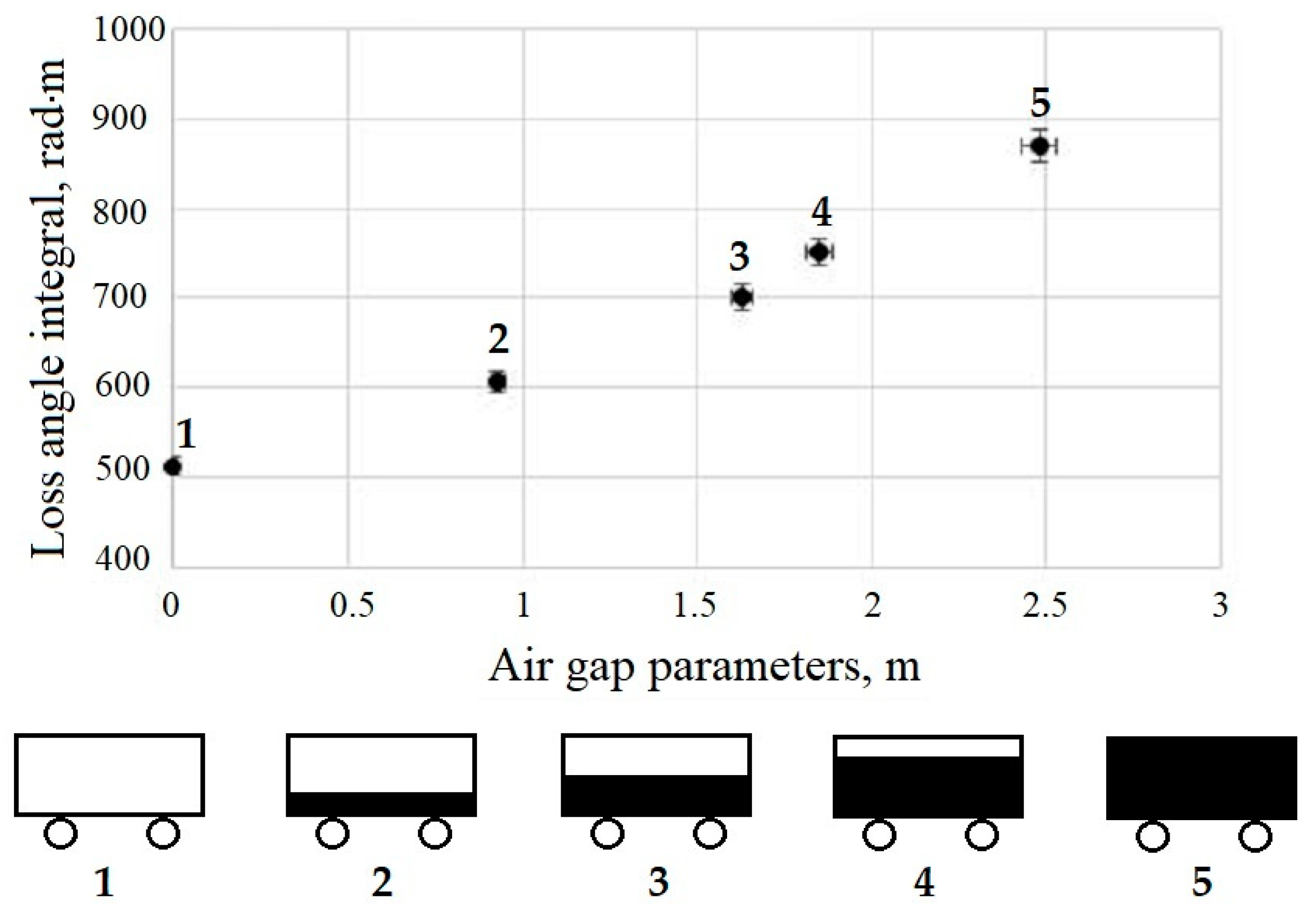
Measurement of integral of dielectric losses envelope curve for ferromagnetic freight of known mass;

(2)

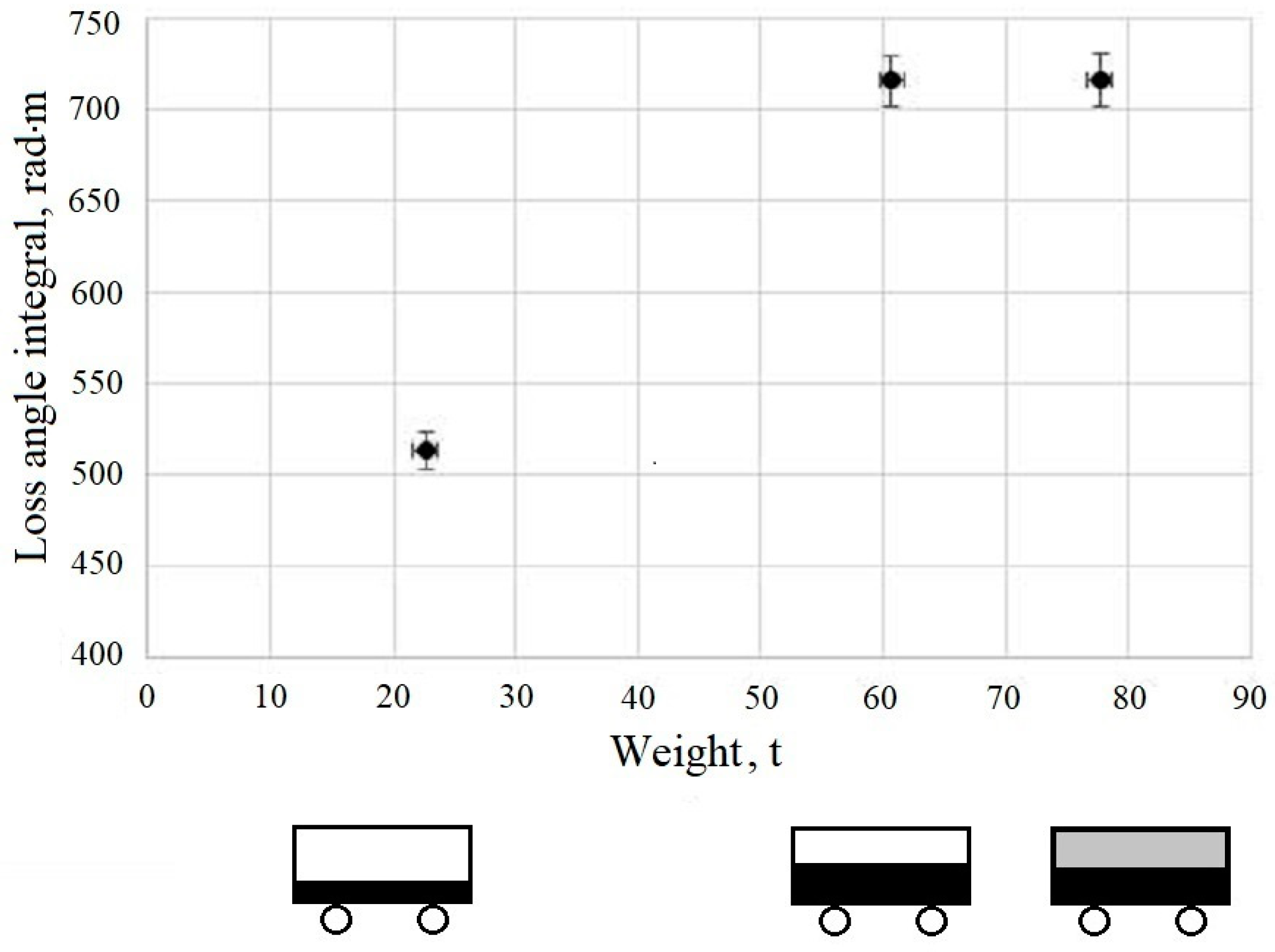
Measurement of integral of dielectric losses envelope curve for same freight with addition of known quantity of non-magnetic material (quartz sand); and

(3)

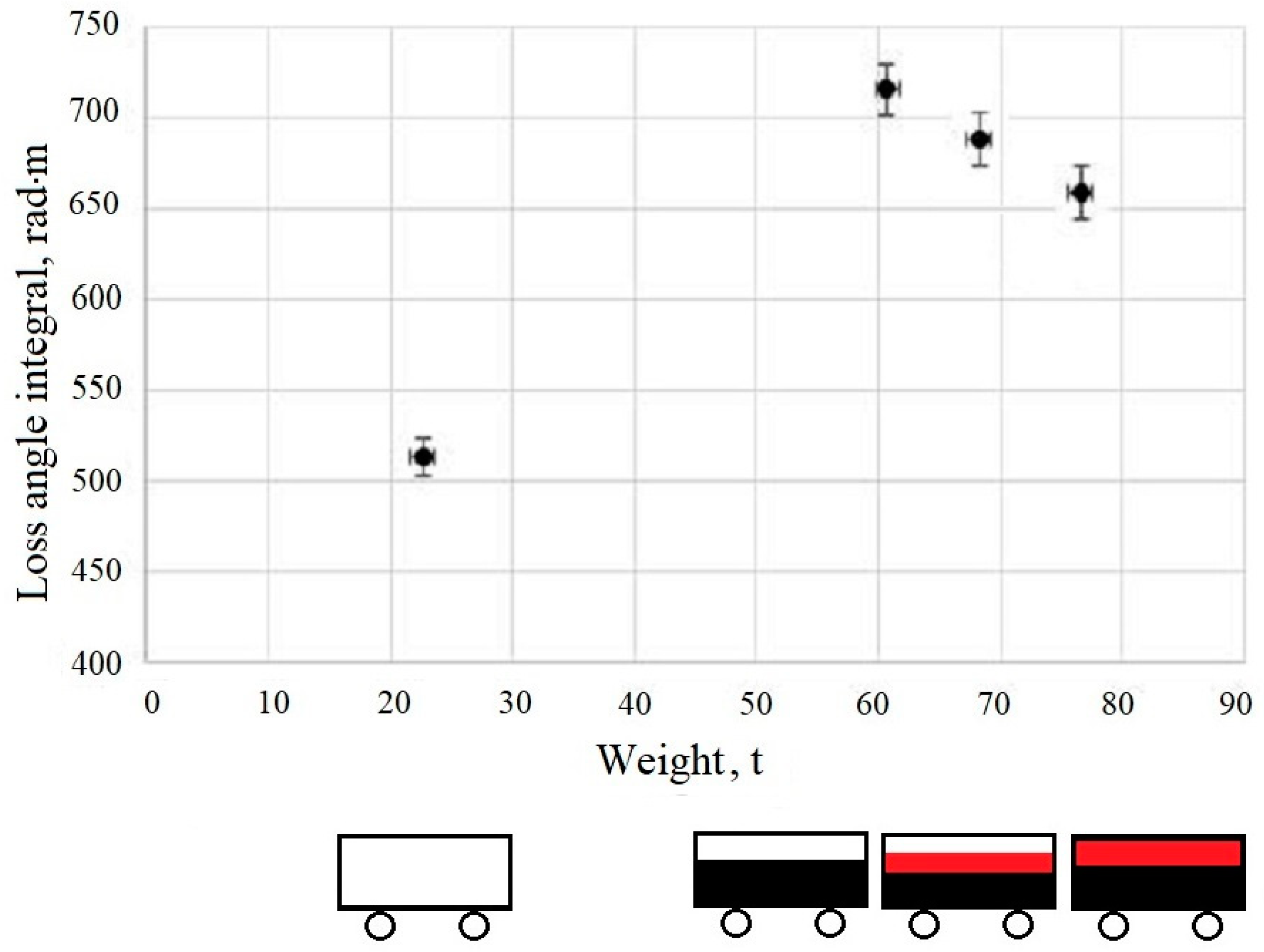
Freight container (railcar of known mass) undergoing the same procedure.

The results are presented in Figure 7. The earth, concrete, polymers, and so on, did not affect the coil parameters.

A somewhat different situation arose when materials with high inductive characteristics, for example, copper or aluminum, were added to a ferromagnetic material. Adding up to 30 wt.% of copper or aluminum lowered the angle of loss of the ferromagnetic material by about 20% (Figure 8).

The figure successively shows the integrals of the loss angle of an empty car, then a car loaded with 35 tons of ferromagnet (black), then cars with 35 tons of ferromagnet loaded sequentially together with 5 and 10 tons of copper (red).

However, this result does not preclude the practical use of the device. Copper and aluminum are much more expensive metals than iron. The addition of non-magnetic inclusions is intended to increase, not reduce, the apparent fraction of a magnetic material according to Equation (29). Therefore, these hidden additives in ferromagnetic material have no practical or economic sense and are not found in practice. Thus, this allows us to calculate the mass fraction of non-magnetic inclusions using Equation (29).

Table 2. Magnitude of non-magnetic inclusions in real scrap metal railcars.

No.	Manufacturer Railcar No.	Type of Scrap (Figure 4)	Total Mass (t)	Empty Car Weight (t)	Wall Height of Railcar (m)	Non-Magnetic Percentage (%)
1	54210059	5A	72.12	22.10	3.2	5.1
2	96632757	3A	85.46	21.85	3.5	3.8
3	96631205	5A	82.67	23.20	3.5	7.2
4	52318037	5A	80.70	22.70	3.5	7.1
5	54035589	5A	78.15	22.20	3.2	5.8
6	56171465	5A	81.10	23.47	3.5	8.9

shows the data on the railcars that passed through the non-magnetic inclusions control unit. There are two types of railcars, differing in wall height (3.2 or 3.5 m). There are also two types of scrap: large and small, noted as 5A and 3A, respectively. The calibrations were experimentally obtained for every type of scrap and railcar.

4. Conclusions

Experimental and theoretical work is underway for more complex tasks, including the definition of unknown parameters, as reflected in Figure 4, Figure 5 and Figure 6.

The need to solve this purely applied task is dictated by a demand from metallurgical enterprises for a solution to this technological problem. Non-magnetic impurities in strategic raw materials cause considerable economic damage. The impossibility of measuring their quantity without fully unloading the car is a technological and legal problem.

The measuring device based on the solenoid, developed as part of our investigations, looks obvious and extremely simple. However, in practice, it had thus far not been created and not a single analogue existed. Therefore, there were no tests with which to compare the technical optimality of our solution. No concept or software algorithm allowed us to evaluate the content of non-magnetic inclusions in a strongly magnetic medium. All previous developments and research focused on the inverse problem—to detect minor impurities of a weakly magnetic metal in a non-magnetic matrix.

The novelty of the proposed solution is that, essentially, its magnetic measurement is an auxiliary parameter characterizing the mass parameters of the system, and the main parameter for the calculation is the mass measured in ordinary weight. On the basis of the described algorithm, the prototype of the railway magnetic scanning device was designed and constructed in one of the metallurgical works.

The presented results show that the chosen measurement and signal processing method allows for a significant expansion of the field of application of the device, such as its use for online monitoring of iron or raw materials transported by railway, or in automotive transport. Other applications are possible, such as the direct control of the quality and the mass of steel products in railway cars. The practical application of the method is based on original software, which allows the calculation of the ratio of the magnetic and non-magnetic components of the load in a railway car by comparing the intensity of the magnetic field perturbation while driving a railway car, and it’s weighing results on a railway car scale. The software package is the intellectual property of the developer.

The technical solutions used in the device are protected by RF Patents 129660 and 120778. UKNV.1–UKNV.3 software was developed using the standard library XPAC SDK, and the special software by ICP DAS was used for analog input high-frequency units.

References

1. Moffat, G.; Williams, R.A.; Webb, C.; Stirling, R. Selective separations in environmental and industrial processes using magnetic carrier technology. Miner. Eng. 1994, 7, 1039–1056. [Google Scholar] [CrossRef]
2. Svoboda, J.; Fujita, T. Recent developments in magnetic methods of material separation. Miner. Eng. 2003, 16, 785–792. [Google Scholar] [CrossRef]
3. Duan, X.; Cheng, J.; Zhang, L. X-ray cargo container inspection system with few-view projection imaging. Nucl. Instrum. Methods Phys. Res. Sect. A 2009, 598, 439–444. [Google Scholar] [CrossRef]
4. Orphan, V.J.; Muenchau, E.; Gormley, J.; Richardson, R. Advanced γ ray technology for scanning cargo containers. Appl. Radiat. Isot. 2005, 63, 723–732. [Google Scholar] [CrossRef] [PubMed]
5. Takahashi, K.; Preetz, H.; Igel, J. Soil properties and performance of landmine detection by metal detector and ground-penetrating radar—Soil characterization and its verification by a field test. J. Appl. Geophys. 2011, 73, 368–377. [Google Scholar] [CrossRef]
6. Volberding, R.W. Cargo container inspection test program at ARPA’s Nonintrusive Inspection Technology Testbed. In Proceedings of the Cargo SPIE’s 1994 International Symposium on Optics, Imaging, and Instrumentation, San Diego, CA, USA, 6 October 1994. [Google Scholar]
7. Gencer, N.G.; Tek, M.N. Electrical Conductivity Imaging via Contactless Measurements. IEEE Trans. Med. Imaging 1999, 18, 617–627. [Google Scholar] [CrossRef] [PubMed]
8. Griffiths, H. Magnetic induction tomography. Meas. Sci. Technol. 2001, 26, 1126–1131. [Google Scholar] [CrossRef]
9. Gursoy, D.; Scharfetter, H. Reconstruction artefacts in magnetic induction tomography due to patient’s movement during data acquisition. Physiol. Meas. 2009, 30, 165–174. [Google Scholar] [CrossRef] [PubMed]
10. Korzhenevskii, A.V.; Cherepenin, V.A. Magnetic induction tomography. J. Commun. Technol. Electron. 1997, 42, 469–474. [Google Scholar]
11. Morris, A.; Griffiths, H.; Gough, W. A numerical model for magnetic induction tomographic measurements in biological tissues. Physiol. Meas. 2001, 22, 113–119. [Google Scholar] [CrossRef] [PubMed]
12. Rudolph, D.J.; Willes, P.M.; Sameshima, G.T. A finite element model of apical force distribution from orthodontic tooth movement. Angle Orthod. 2001, 71, 127–131. [Google Scholar] [CrossRef] [PubMed]
13. Hakim, N.S.; King, A.I. A three-dimensional finite element dynamic response analysis of a vertebra with experimental verification. J. Biomech. 1979, 12, 277–292. [Google Scholar] [CrossRef]
14. Smith, I.M.; Griffiths, D.V.; Margetts, L. Programming the Finite Element Method, 5th ed.; John Wiley & Sons: Hoboken, NJ, USA, 2013. [Google Scholar]
15. Vonsovskiy, S.V. Magnetism; Nauka: Moscow, Russia, 1971. (In Russian) [Google Scholar]
16. Grossi, M.; Riccò, B. Electrical impedance spectroscopy (EIS) for biological analysis and food characterization: A review. J. Sens. Sens. Syst. 2017, 6, 303–325. [Google Scholar] [CrossRef]
17. Callegaro, L. Electrical Impedance: Principles, Measurement and Applications; CRC Press: Boca Raton, FL, USA, 2016. [Google Scholar]
Figure 1. Experimental setup diagram. 1. Railway car, 2. Measuring coil system, 3. Building construction elements, 4. Platform car weights, 5. Signal reception and processing system.
Applsci 09 02001 g001
Figure 2. Experimental envelope function of a core consisting of 10 consecutively connected railcars with the ferromagnetic freight.
Applsci 09 02001 g002
Figure 3. Dependence of the loss angle integral on the air gap parameters.
Applsci 09 02001 g003
Figure 4. The dependence of the loss angle integral on mass for the different types of cargo with a fixed air gap. The color of the car in the explanation corresponds to the color of a straight line on the graph in the legend.
Applsci 09 02001 g004
Figure 5. The dependence of the loss angle integral on a vertical position of a ferromagnetic object of constant mass.
Applsci 09 02001 g005
Figure 6. The change in the instantaneous values of the angle of loss at different locations of the magnetic load.
Applsci 09 02001 g006
Figure 7. Dependence of loss angle integral on core mass with different proportion of magnetic and non-magnetic components.
Applsci 09 02001 g007
Figure 8. The dependence of the loss angle integral on the core mass with different proportions of ferromagnetic material and copper.
Applsci 09 02001 g008