Predictive Optimization of the Heat Demand in Buildings at the City Level

Abstract

Easily adaptable indoor temperature and heat demand models were applied in the predictive optimization of the heat demand at the city level to improve energy efficiency in heating. Real measured district heating data from 201 large buildings, including apartment buildings, schools and commercial, public, and office buildings, was utilized. Indoor temperature and heat demand of all 201 individual buildings were modelled and the models were applied in the optimization utilizing two different optimization strategies. Results demonstrate that the applied modelling approach enables the utilization of buildings as short-term heat storages in the optimization of the heat demand leading to significant improvements in energy efficiency both at the city level and in individual buildings.

1. Introduction

According to a recent study by Connolly [1], heating in buildings presents the largest energy demand in 15 EU countries, and it is also higher than cooling demand in all 28 EU countries. At the same time, the peak demand for heating is considerable. In heat production, peak loads occur when the heat demand exceeds the capacity of the power plants. During the peak loads, oil powered reserve capacity is typically needed. This raises production costs and environmental impact for the energy company and creates a strong economic and environmental incentive to find ways to cut peak loads and reduce the use of oil. Reducing peak loads would also enable more buildings to be connected to the heating network. This article presents simulation studies employing previously developed, easily adaptable indoor temperature and heat demand models to demonstrate their applicability to predictively optimize the heat demand and to cut the peak loads by utilizing buildings as short-term heat storage. The applied modelling approach is argued to provide a cost-effective way to implement predictive optimization and to improve energy efficiency in heating.

One way to cut peak loads is by means of demand side management (DSM). The term was introduced by Gellings [2] in the 1980s. He defined DSM as activities aimed to influence the electricity use of customers in ways that will produce desired changes in the load shape. Consequently, the majority of the published literature discusses DSM in the context of electricity [3,4,5]. However, DSM is equally applicable to district heating. In [4], three possible ways to achieve the change in the end-user energy consumption with DSM are described. The first way is to reduce the energy consumption during the peak loads. In case of heating, this could mean a temporary loss of comfort. Secondly, the energy consumption could be shifted to a different period of time. This would mean that the buildings are pre-heated before the peak loads. The third way is to use on-site generated energy for example heat pumps, solar collectors, or even fireplaces. All these ways can be efficiently utilized if the heat consumption can be predicted.

The authors have studied a concept for cutting the peak loads and optimizing the heat demand and the main idea is to utilize buildings as short-term heat storages [6]. It is well known that in this way the peak loads can be cut, the indoor temperature swings can be reduced and the time of heat demand can be shifted [7,8,9,10,11]. However, as the predictive control for buildings has gained popularity, the time used for modelling has been identified as one of the most important factors when considering the total implementation work [12,13]. Model Predictive Control (MPC) is currently one of the most studied control strategies for buildings and it has been reported that the modelling work can be as high as 60% of the total MPC implementation work [12,14]. Considering the above, easily applicable models would make the implementation of advanced model-based control and optimization methods significantly more cost-effective.

Fang and Lahdelma [15], Short et al. [16], and Powell et al. [17] all optimized heat production in the district heating system assuming a central heat storage unit. In this work, the aim was to study how the heat demand can be optimized and how much peak loads can be cut at the city level by modelling each individual building to enable the utilization of their thermal storage capacity. Motivation for this comes from the fact that the heat storage capacity of buildings offers effective and efficient way to store heat [18,19]. Moreover, the capacity already exists, and only proper ways to utilize that are needed. It is also argued that the solution is more cost-effective as there are no large investment costs involved like in the case of large central heat storage solutions. Furthermore, Razani and Weidlich [20] found that decentralized heat storage was most energy efficient when they optimized the configuration of heat storage in the district heating system. Regardless, the utilization of the buildings as the short-term heat storage provides a valuable tool to further improve the flexibility and energy efficiency in heating. It has been estimated that through optimized operation and management 20–30% savings in building energy consumption are possible without any hardware changes in the building [21].

There have been some efforts in utilizing the thermal mass of buildings in peak load cutting at the large scale. Guelpa et al. [22] performed peak load cutting utilizing the heat storage of buildings without building models. Reduction of 5.8% in peak loads was achieved. However, the changes in the heating loads had to be small to ensure minimal changes in the indoor temperature. Larger changes in heat loads would require the use of building models to maintain the indoor temperature at the desired level as Verda et al. [23] did in their study. However, the calculation of the parameters of the applied building model needed experimental data that would be laborious to collect and limited the applicability of the model. Verrilli et al. [24] performed peak load cutting in a residential heating system with 50 buildings utilizing DSM algorithm. The algorithm determined the buildings where the heating should completely be cut off and then the decrease in the indoor temperature of the buildings was predicted with Newton’s cooling law considering the thermal time constant of the buildings. However, they only considered cutting the heating completely off. This leads to the suboptimal use of buildings thermal mass, as only buildings with high enough indoor temperatures to withstand the complete cut off of heating will participate in the peak load cutting. Moreover, the estimation of the building time constant is not an easy matter. Kontu et al. [25] applied DSM for three different-sized district heating systems considering different building groups. They emphasize the complexity of the matter and that it is affected by many factors such as the building structure and the outdoor and indoor conditions. However, their study did not include models of any kind for the buildings to take into account the dynamics of the indoor environment.

In previous studies, the authors have developed models for indoor temperature and heat demand forecast for buildings to overcome the current modelling issues hindering the application of the models in a large scale [26,27]. However, the optimization was not considered in these works. In another work, peak load cutting was studied in two different buildings utilizing the indoor temperature model and it was found that buildings can have very different heat storage capabilities and the energy savings or peak load cuts achieved in a single building are not necessarily the indication of the larger scale performance [28]. Consequently, the optimization of individual buildings alone is of no interest when considering the overall benefits to the energy system [29,30]. Therefore, in this work, the two developed forecast models are applied together in the predictive optimization of the heat demand at the city level. Furthermore, Reynolds et al. [31] have reported that most of the literature relating to the district level optimization concentrate on the optimal supply of a district assuming the energy demand of the buildings as known, perfectly predicted, and unalterable. In this work, the developed models enable the utilization of the heat storage capacity of the buildings allowing to alter the heat demand profile of the buildings making them active participants in the energy systems. All this is possible as the models are accurate and easily applicable to different buildings offering a valuable tool for the optimization of energy networks to improve energy efficiency.

In the next section, the measurement data used in the simulations is described. The applied models and their parameter estimation methods along with the predictive optimization methods are explained in Section 3. The simulation results are presented in Section 4 and discussed in Section 5. Finally, Section 6 contains conclusions.

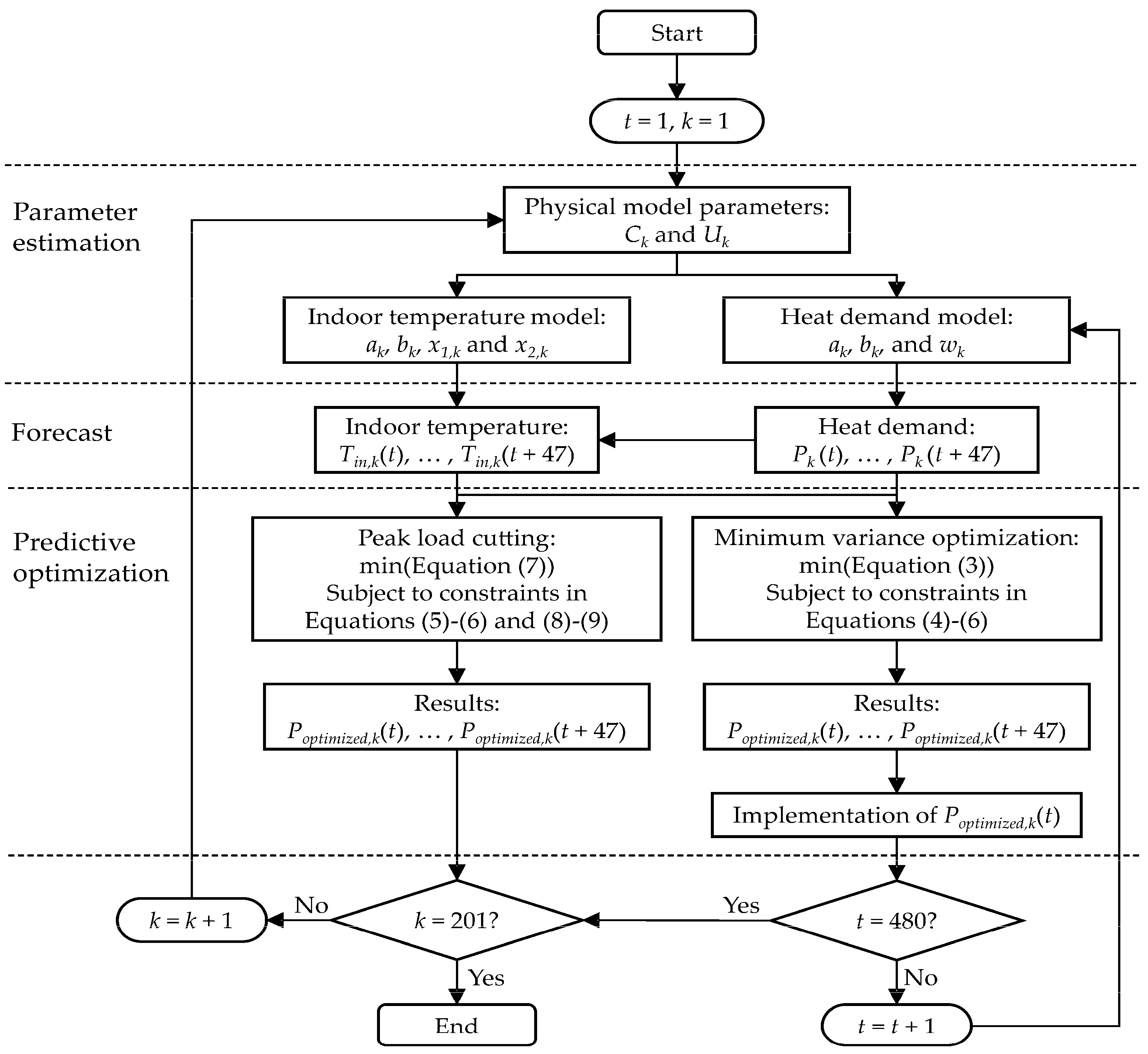
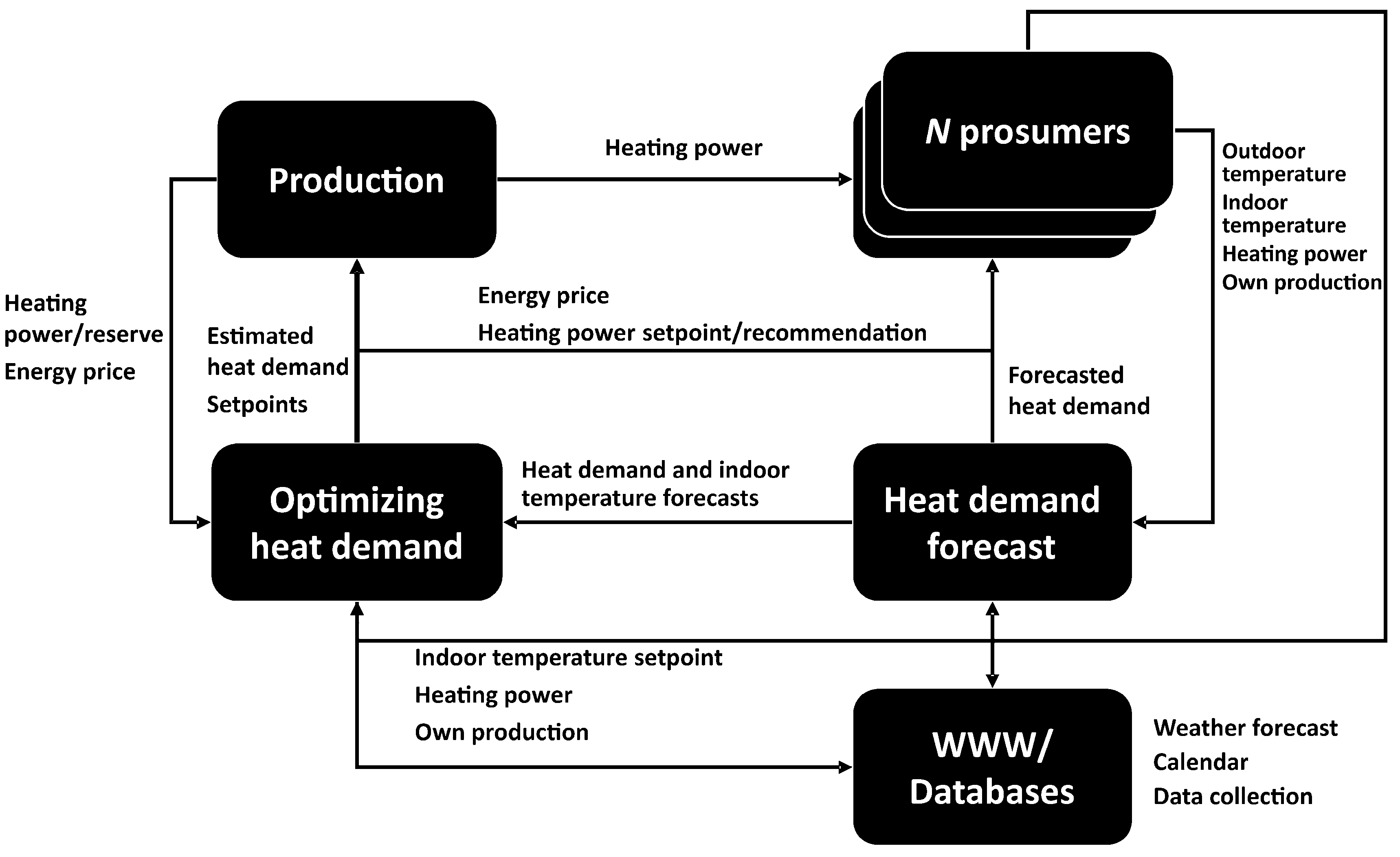
2. Measurement Data

The district heating data of the city of Jyväskylä, Finland, from January 2013 was used for the parameter estimation of the models and for the optimization simulations. The data was provided by the local heating utility and included the hourly measured heat consumption (P) and volume (V) for individual buildings together with the hourly measured outdoor temperature (T_out). The same outdoor temperature measurements were used for all the buildings as local outdoor temperature data were not available. Outdoor temperature range was from −26.7 °C to + 2.1 °C with median value being −6.5 °C. For the simulation studies, the 201 largest district heat consumers among the apartment buildings, schools, and commercial, public and office buildings were chosen as these kinds of buildings are the most likely to be included in the DSM. The combined heat consumption of these 201 buildings amounted to 32% of the total heat consumption of the Jyväskylä district heating system. Measurement data for the buildings is presented in

Table 1. Measurement data from January 2013 for 201 buildings in the city of Jyväskylä, Finland.

Building Group	Number of Buildings	Range of V [m3]	Median V [m3]	Range of P [kW]	Median P [kW]
Apartment buildings	82	9791–87,916	21,615	0–960	170
Schools	35	8380–250,830	29,750	0–3720	270
Commercial, public and office buildings	84	9969–169,372	35,247	0–2200	245

.

3. Methods

Previously developed indoor temperature and heat demand models for buildings were utilized to forecast the indoor temperature and heat demand in individual buildings. Two different optimization strategies were utilized in the predictive optimization of the heat demand in 201 buildings. First, the parameters of the forecast models were estimated for each building utilizing hourly recorded measurement data. Then, the heat demand and indoor temperature in individual buildings were forecasted for the next 48 h. Finally, two different optimization strategies, minimum variance optimization and peak load cutting, were utilized to optimize the hourly heat demand in each building. In minimum variance optimization, the variance of the heat demand of individual buildings were minimized. In peak load cutting, the hourly heat demands of individual buildings were cut during the defined hours. In both cases, the indoor temperatures were kept between defined limits and the total heat demands were not allowed to increase. The forecast models, parameter estimation and predictive optimization strategies are further discussed in the next sections.

3.1. Forecast Models

For indoor temperature forecast, a previously developed dynamic model was applied and is presented here in Equation (1) [26]:

$${\widehat{T}}_{in,k}\left(t\right)=a_k\{T_{in,k}\left(t-1\right)+\frac{\Delta t}{C_k}\left[x_{1,k}{P}_k\left(t-1\right)+x_{2,k}{P}_k\left(t-3\right)-U_k\left(T_{in,k}\left(t-1\right)-T_{out,k}\left(t-1\right)\right)\right]\}+b_k,$$

(1)

where k denotes an individual building, a_k, b_k, x_1,k, and x_2,k are estimated model parameters and C_k (kJ/K) and U_k (kW/K) are building specific physical constants the thermal capacity and the heat loss coefficient respectively. ${\widehat{T}}_{in,k}\left(t\right)$ is the forecasted indoor temperature at time t and T_in,k(t − 1) is the indoor temperature at time t − 1. Δt is the time step between the values ${\widehat{T}}_{in,k}\left(t\right)$ and T_in,k(t − 1) namely 3600 s (1 h). P_k(t − 1) and P_k(t − 3) are the heat demands at times t − 1 and t − 3 respectively. T_out,k(t − 1) is the outdoor temperature at time t − 1.

The applied heat demand model is presented in Equation (2) [27]:

$${\widehat{P}}_k\left(t\right)=\left\{a_k\left[P_k\left(t-1\right)-U_k\left(T_{in,k}\left(t\right)-T_{out,k}\left(t\right)\right)\right]+b_k\right\}+w_k\left(t\right),$$

(2)

where a_k and b_k are estimated model parameters, ${\widehat{P}}_k\left(t\right)$ is the forecasted heat demand at time t, P_k(t − 1) is the heat demand at time t − 1 and w_k(t) is the value of the residual model at time t. The residual model is the hourly average of the residuals of the output from the dynamic model (inside the brackets in Equation (2)) and the measured heat demand.

When forecasting the indoor temperature and heat demand, the future values are calculated recursively using previously forecasted indoor temperatures and heat demands as inputs. Outdoor temperature forecast should also be used but in this study the simulations were done using measured outdoor temperatures. In previous studies, the average modelling error for the indoor temperature model was below 5% [26] and for the city level heat demand forecast it was 4% [27]. For more in-depth discussion on the applied models and their validation, readers are referred to [26] and [27]. However, it must be noted that the models were developed for the optimization of the heat demand at the city level. Therefore, they have low amounts of free parameters and input variables to enable the ease of application to the whole building stock comprising hundreds or even thousands of buildings.

3.2. Parameter Estimation

The parameters a and b of the heat demand model (Equation (2)) were estimated using one week of measured heat demand and outdoor temperature data as in [27]. On the other hand, as in this work there were hundreds of buildings studied and there were no indoor temperature measurements available from these buildings, the measured indoor temperature could not be used for the estimation of the parameters a, b, x₁, and x₂ of the indoor temperature model (Equation (1)) as in [26]. Therefore, the indoor temperature of the buildings had to be simulated.

3.2.1. Simulating the Indoor Temperature

Only the measured heat demand and outdoor temperature were used for the simulation of the indoor temperature in the buildings. The parameters a, b, x₁ and x₂ of the indoor temperature model (Equation (1)) were estimated by applying constraints to the simulated indoor temperature. By analyzing known indoor temperatures in different buildings the simulated indoor temperature was constrained between 16 °C and 23 °C and the standard deviation of the simulated indoor temperature was constrained between 0.2 °C and 1.1 °C. The parameters were first estimated using one week of measured heat demand and outdoor temperature data. Then, using the estimated parameters, the indoor temperature was simulated for another two days. In both cases, the indoor temperature and its standard deviation were checked to ensure it was between the defined limits. If in both cases this was true, the parameters would be accepted and the model was used for the optimization simulations. Otherwise, the parameter estimation was performed again. For the parameter estimation, the simulated annealing algorithm from the Global Optimization Toolbox of MATLAB^® was used. As there were no real indoor temperature measurements available, the assumption for the optimization studies was made that the simulated indoor temperature is the set point temperature in the buildings. Furthermore, as the indoor temperature model defines the heat storage capacity of the buildings and as there were no measured indoor temperatures to calibrate the model, multiple sets of parameters for the indoor temperature model were estimated for each building.

3.2.2. Physical Model Parameters

In the previous work [27], the physical model parameter U was estimated using the volume of the building by fitting a power function of form f(x) = d × x^p to the data of the known volumes and values of parameter U. This way the value of the parameter could be estimated easily for thousands of buildings. In this work, also the physical model parameter C needs to be estimated for the indoor temperature model. A similar method for the estimation of the parameter C is used as in the case of parameter U in [27]. The resulting equation is C = 5896 × V^0.6059, where V (m³) is the volume of the building.

3.3. Predictive Optimization of the Heat Demand

3.3.1. Minimum Variance Optimization

The cost function for minimum variance optimization minimized the variance of the heating power while not increasing the total heat demand and keeping the indoor temperature between defined limits as follows:

$$J_k=var\left(P_{optimized,k}\right)+P_{Penalty,k}+{{\displaystyle \sum }}_{t=1}^N{T}_{Penalty,k}\left(t\right),$$

(3)

where P_optimized,k is the heating power during the optimization period, N is the number of hours in the optimization period, P_Penalty,k is the penalty for an increase in total heat demand and T_Penalty,k is the penalty for indoor temperature outside the defined limits. The optimization was subject to the following constraints:

$${{\displaystyle \sum }}_{t=1}^N\left(P_{optimized,k}\left(t\right)-P_{forecasted,k}\left(t\right)\right)\le 0,$$

(4)

$$P_{min,k}\left(t\right)\le P_{optimized,k}\left(t\right)\le P_{max,k}\left(t\right)foreacht=1,\dots ,N,$$

(5)

$$T_{in,min,k}\left(t\right)\le T_{in,optimized,k}\left(t\right)\le T_{in,max,k}\left(t\right)foreacht=1,\dots ,N,$$

(6)

where P_optimized,k(t) and P_forecasted,k(t) are the optimized and forecasted heat demands at time t, respectively. P_min,k(t) and P_max,k(t) are minimum and maximum heating powers at time t and T_{in,optimized,k}(t), T_in,min,k(t) and T_in,max,k(t) are optimized, minimum and maximum indoor temperatures at time t, respectively.

The heat demand was optimized for 480 h in each individual building applying the receding horizon or sliding time window approach [15,32]. In each iteration, the heat demand and the indoor temperature were forecasted for 48 h and the optimization result of the first hour was saved meaning that one-hour control horizon was assumed. Then the 48-h forecasting horizon was advanced one hour and optimized again, saving the result of the first hour, until results for 480 h were achieved. The variance of the heating power was minimized for the 48-h forecast horizon and for all the past results as illustrated in Figure 1, using the pattern search algorithm from the Global Optimization Toolbox of MATLAB^®. In addition, the heat demand was not allowed to increase meaning that the optimized heat demand had to be equal to or smaller than the forecasted heat demand (Equation (4)) and the hourly heating power was constrained between building specific maximum and minimum values (Equation (5)) evaluated from the measured data. During the optimization, the indoor temperature was allowed to change between −0.5 °C and +1.0 °C from the simulated indoor temperature (Equation (6)) enabling the use of buildings as short-term heat storage.

3.3.2. Peak Load Cutting

In the earlier work, the cost function for peak load cutting minimized the heat demand [28]. However, in the case were no measured indoor temperatures are available and with the assumption that the simulated indoor temperature is the set point temperature, minimizing the heat demand would mean that the indoor temperature would just be decreased to the minimum level. Therefore, in this work the cost function for peak load cutting minimized the difference between the forecasted and the optimized heat demand keeping the change in the total heat demand at minimum:

$$J=|{{\displaystyle \sum }}_{t=1}^N(P_{forecasted,k}-P_{optimized,k})|+{{\displaystyle \sum }}_{t=1}^N\left(P_{ChangePenalty,k}\left(t\right)+T_{Penalty,k}\left(t\right)\right),$$

(7)

where P_{changePenalty,k} is the penalty for too large hourly changes in the heating power. The optimization was subject to the constraints in Equations (5) and (6), and the following:

$$\left|P_{optimized,k}\left(t\right)-P_{optimized,k}\left(t-1\right)\right|\le P_{change,k},$$

(8)

$$0.3P_{forecasted,k}\left(t\right)\le P_{optimized,k}\left(t\right)\le P_{forecasted,k}\left(t\right)$$

(9)

where P_change,k is the building specific maximum hourly change in heating power. The heating power was constrained to be 30–100% of the forecasted heat demand for the hours when the peak load cutting was realized depending on the heat storage capability of the building. This means that a maximum of 70% peak load cut was assumed to be possible. This is consistent with the results in [28]. The pattern search algorithm from the Global Optimization Toolbox of MATLAB^® was utilized in the optimization.

4. Results

The optimization was performed as illustrated in Figure 2. First the physical parameters C and U were calculated (Section 3.2.2). Then the model parameters for the indoor temperature and heat demand models (Equations (1) and (2)) were estimated. Next, the indoor temperature and heat demand were forecasted, and finally the predictive optimization was performed. In each optimization cycle, there were 48 real number variables (heat demand for each hour of the 48-h forecast horizon) for each building subject to hard bounding constraint in Equation (5). The hourly indoor temperature was subject to bounding constraint in Equation (6) inflicting penalty (T_Penalty) if breached. In addition, for minimum variance optimization, the total heat demand for the 48 h was subject to inequality constraint in Equation (4) inflicting penalty (P_Penalty) if breached. For peak load cutting the hourly heat demand was subject to the inequality constraint in Equation (8) inflicting a penalty (P_{changePenalty}) if breached. Also, for the peak load cutting period, the hourly heat demand was subject to the bounding constraint in Equation (9). The indoor temperature model parameters were estimated only once for each building at the beginning of a simulation run. For the 480-h minimum variance optimization (Section 3.3.1), the heat demand model parameters were updated in each iteration as presented in Figure 2.

All the computations were performed in MATLAB^® environment on a standard PC with Intel^® Core i7 processor with 3.4 GHz speed and 8 GB of RAM. As the optimization was performed separately for each building, local parallel computing in MATLAB^® was utilized. Calculation time for one optimization cycle including the estimation of parameters for the heat demand model was approximately four minutes.

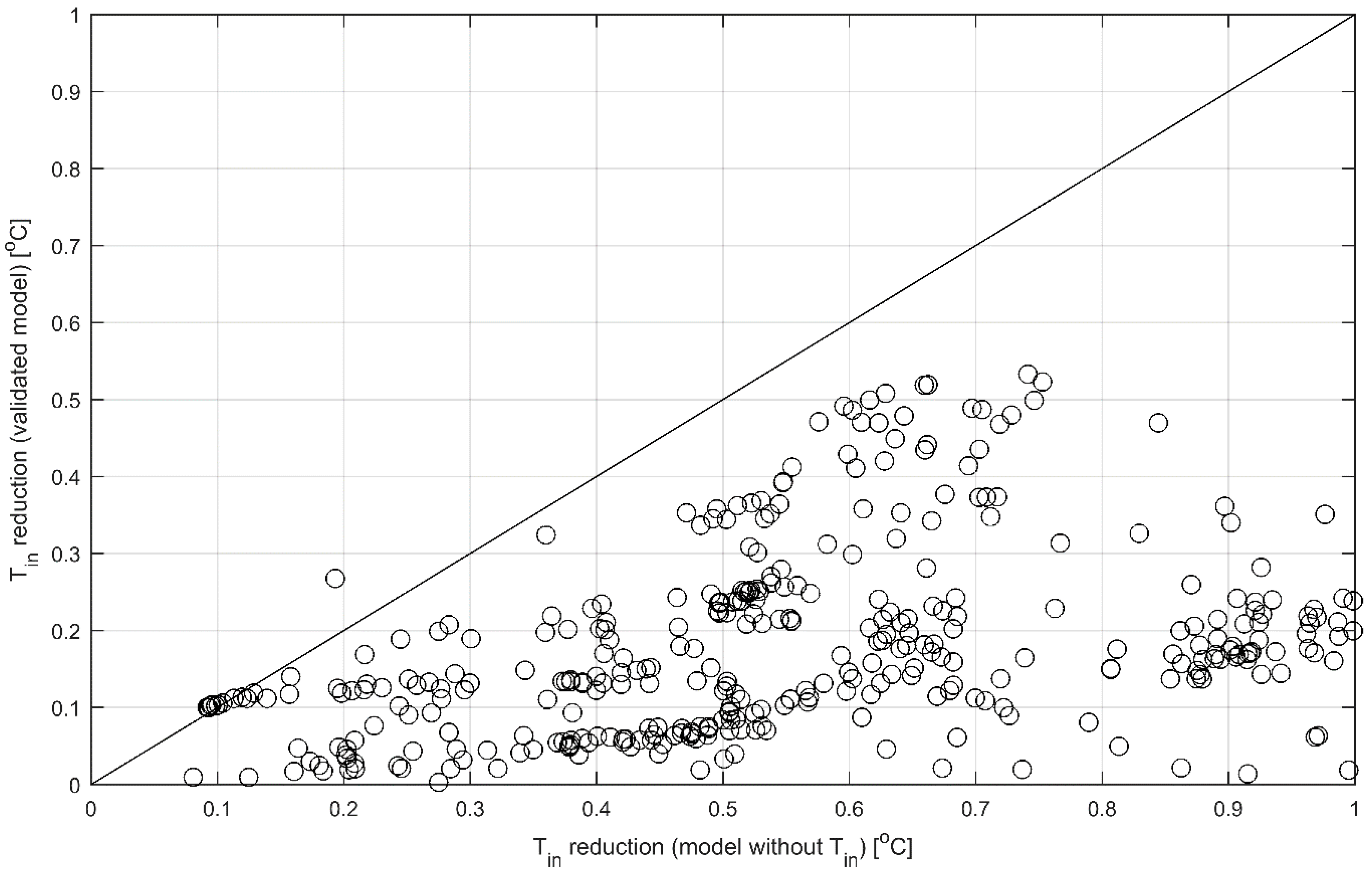
4.1. Validation of the Parameter Estimation Method for Indoor Temperature Model

To ensure the applicability of the parameter estimation method for the indoor temperature model, it was tested with the data of five different buildings presented in [26] where measured indoor temperatures were used for the parameter estimation. Parameters of the indoor temperature model (Equation (1)) were estimated using the method described in Section 3.2 utilizing four 100-h identification data sets and predicting indoor temperatures for four 28-h validation data sets presented in [26]. This amounted to four different parameter sets for all five buildings including the physical constants C and U. Heating power was then decreased by 30% for the validation periods and indoor temperature was predicted again. The change in indoor temperature was then compared between the two models and results are presented in Figure 3.

As in this study, the change in modelled indoor temperature was restricted between −0.5 and +1 °C. The results for up to 1 °C absolute change are of interest and are shown in Figure 3. The model whose parameters are estimated using the method described in Section 3.2 overestimates the change in indoor temperature when compared with the indoor temperature model identified and validated in [26]. Therefore, also taking the error of the indoor temperature model into account, it can be concluded that up to 1 °C changes in the simulated indoor temperature are realistic and safe to make and are not going to compromise the indoor temperature in the buildings.

4.2. Optimization of the Heat Demand

4.2.1. Minimum Variance Optimization for 480 h

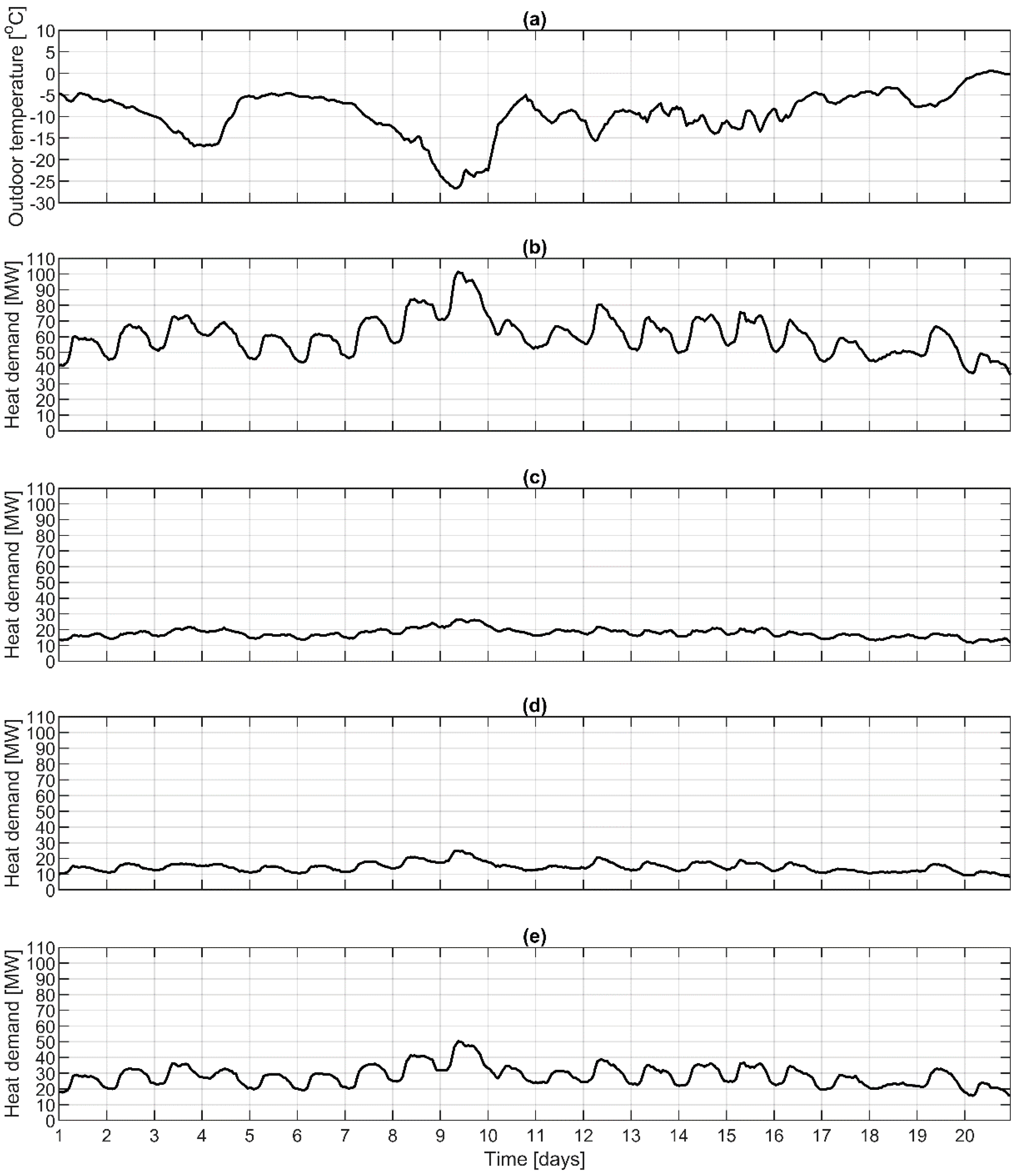
Figure 4 shows the total measured heat demand for 201 buildings and for different building groups and the measured outdoor temperature for the 480-h time period. The heat demand follows the outdoor temperature, but daily variation in the heat demand can also be seen. This daily variation is caused by the lowered heating power in many of the buildings during the night. Daily variation is somewhat smaller during the weekends because many of the buildings are unoccupied. Days 3–4, 10–11, and 17–18 are weekends in Figure 4.

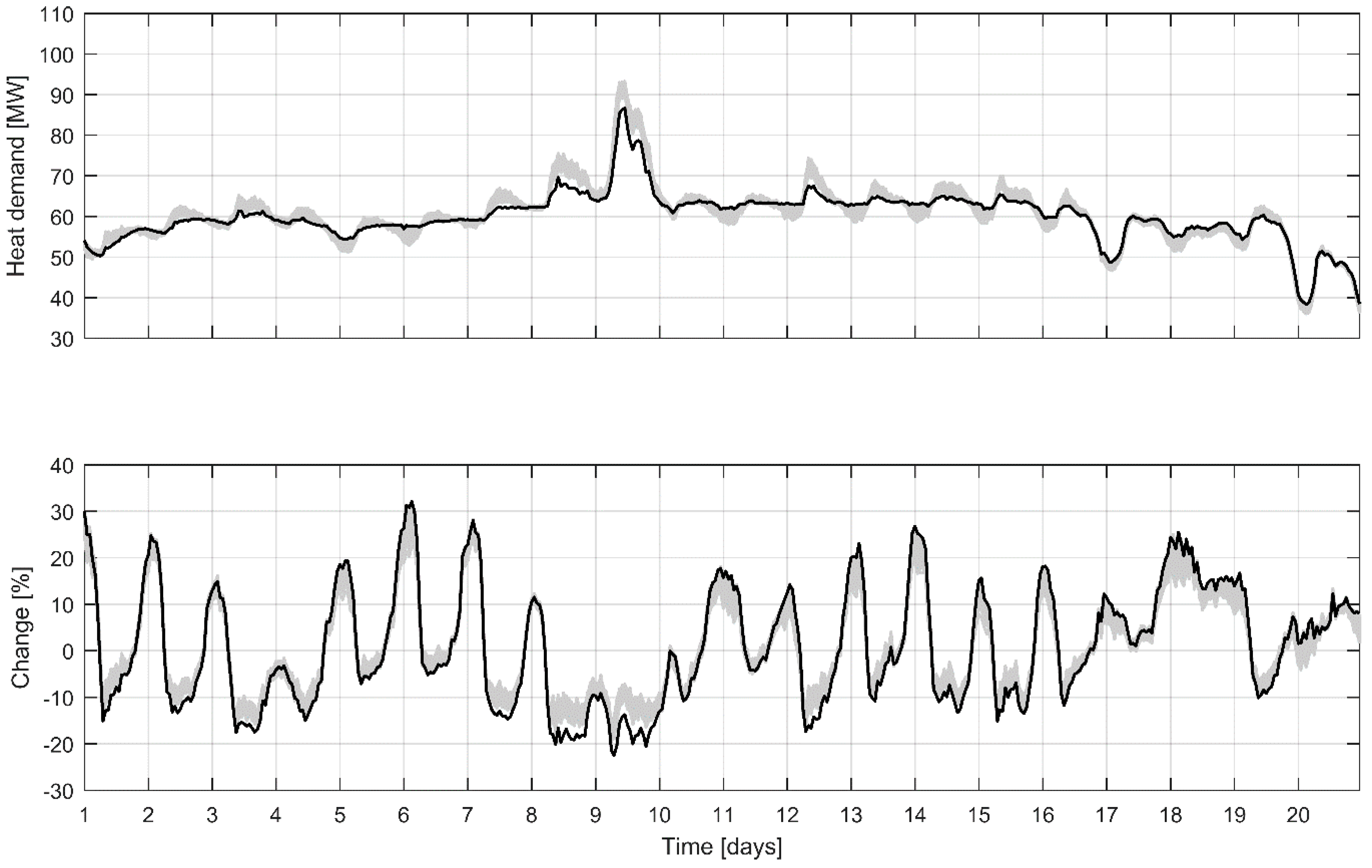
Four different sets of parameters for the indoor temperature model (Equation (1)) were estimated for each of 201 buildings. Then the 480-h time period was optimized in each building as presented in Figure 2 and discussed in Section 3.3.1. In Figure 5, 1000 random combinations of optimization results are presented. Each combination contains results using one of the four estimated indoor temperature models for each building. The optimized total heat demand was in all cases 0.2–4.5% lower than the original measured total heat demand and the maximum heat demand was reduced 8–11%.

The result with the lowest variance of the heat demand in each building is also shown in Figure 5. In that case, the optimized heat demand was 1.1% lower, and at the maximum heat demand was reduced by 14%, which corresponds to a 4.9% reduction in the total heat demand for the whole district heating system. Compared with the measured total heat demand in Figure 4b, the applied optimization method can be seen to smoothen the heat demand by increasing the heat demand during lower demand and by decreasing the heat demand during high demand. This is possible by utilizing the heat storage capacity of the buildings.

As the predictive optimization relies on the accuracy of the heat demand forecast, mean absolute percentage error (MAPE) and Pearson correlation coefficient (r) for the heat demand forecast of individual buildings are presented in

Table 2. The number and percentage of individual buildings with mean absolute percentage error (MAPE) lower than 30% and Pearson correlation coefficient (r) greater than 0.5 for the 48-h heat demand forecast.

r	MAPE
	<30%	<25%	<20%	<15%	<10%	<5%
>0.5	181 (90.0)	177 (88.1)	170 (84.6)	161 (80.1)	128 (63.7)	47 (23.4)
>0.6	173 (86.1)	170 (84.6)	163 (81.1)	154 (76.6)	126 (62.7)	47 (23.4)
>0.7	163 (81.1)	160 (79.6)	155 (77.1)	148 (73.6)	122 (60.7)	47 (23.4)
>0.8	117 (58.2)	115 (57.2)	112 (55.7)	108 (53.7)	87 (43.3)	38 (18.9)
>0.9	47 (23.4)	47 (23.4)	45 (22.4)	43 (21.4)	31 (15.4)	11 (5.5)

. For individual buildings, MAPE varied from 3.6–59.8% and r from 0.19–0.97 for the 48-h ahead heat demand forecast during the 480-h optimization period. However, the average MAPE and r were 10.2% and 0.78, respectively. For 122 (60.7%) buildings, the MAPE was lower than 10% while r was greater than 0.7. There were 17 buildings with r lower than 0.5. Most of these buildings had heating power that varied highly on hourly intervals making it hard to forecast the exact heat demand and this lowered the r value. In 22 buildings, the MAPE was over 20%. These buildings included some of the ones with low correlation values, but in general these buildings had a clear day and night cycle in their heat demand profile and the model overestimated the heat demand during the day-time while underestimating it during the night-time.

Although the total heat demand was a few percent lower in all the simulations, in some individual buildings the heat demand actually increased. This occurred in 27 buildings with all the applied indoor temperature models and in 110 buildings with some of the applied indoor temperature models. The median increase was 2.1% and at most the increase was 16.8%. An increase of a few percent in heat demand may seem small, but considering that the studied buildings have high heat demands, it could mean a significant increase in heating costs. The increase can be explained by the error in the predicted heat demand.

When considering the optimization results that produced the minimum heat demand in each building, the maximum total heat demand was decreased 11% and the total heat demand during the 480-h optimization period was 4.4% lower than the original measured total heat demand.

The applied optimization method does not fully utilize the heat storage in buildings, as can be seen in Figure 5, when considering the highest heat demand of the period during the day nine. It can be seen that the heat demand is decreased also in the early morning hours before the peak, which would affect the amount of the peak load cut during the high demand. This is due to the fact that the formulation of the optimization problem is not directly intended for peak load cutting although daily peak loads are cut as seen in Figure 5.

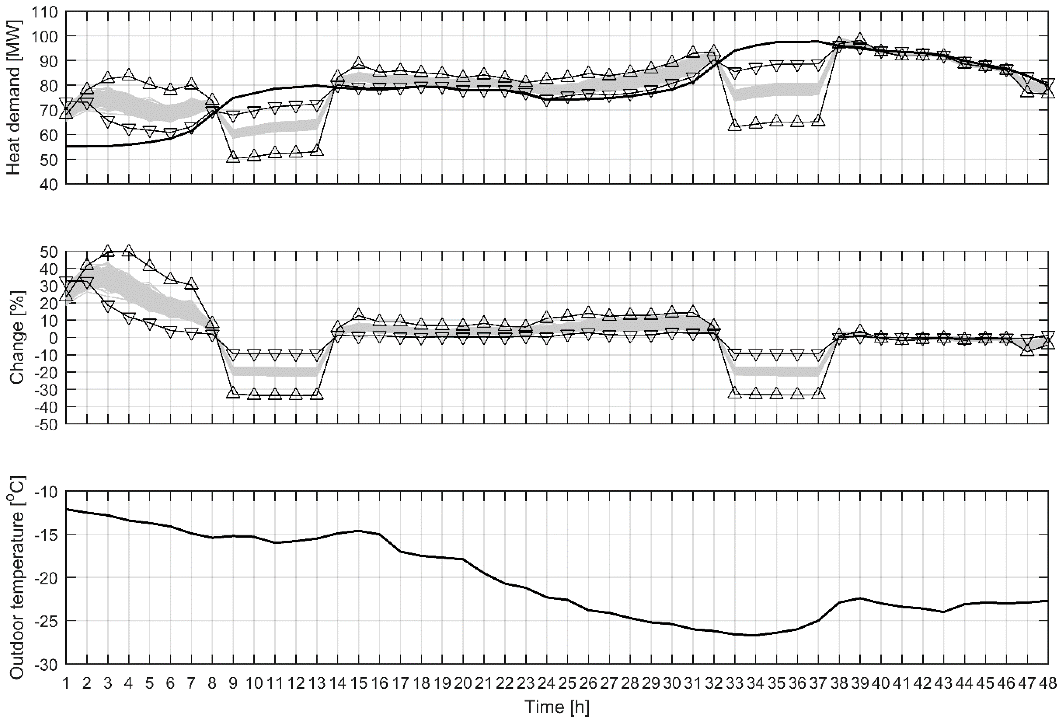
4.2.2. Cutting of Peak Loads

To examine the full peak load cut capacity, days eight and nine from the 480-h optimization period were chosen for further study as they contain the highest consumption peak. The peak load cutting for this 48-h period was performed as discussed in Section 3.3.2 and presented in Figure 2. Six different sets of parameters for the indoor temperature model (Equation (1)) were estimated for each of the buildings as this affects to their heat storage capability. The results of 1000 randomly chosen combinations of optimization results including the largest and lowest peak cuts are presented in Figure 6. Each combination contains results using one of six estimated indoor temperature models for each of the buildings. As large as 33% peak load cuts in total heat demand of 201 buildings were achieved between 8 and 12 a.m. At 10 a.m. on the second day, this cut corresponded to 30 MW reduction in heating power. That amount of reduction in heat load will have a significant effect on city level. However, most of the time the peak load cut was 16–22% meaning 17–21 MW reduction in heat load. The minimum peak load cut was 9% corresponding to 9 MW reduction. Furthermore, it can be seen how the heat demand is shifted from morning to night. In the indoor temperature of buildings, this means that the indoor temperature is increased during the night and then let to drop during the peak load cutting. It is important to notice that there are no additional peaks in the heat demand after the peak load cutting period, rather the heat demand returns to the original level. This means that the indoor temperature will slowly rise to the set point always staying between the defined limits.

Table 3. Peak load cut in different building groups.

Building Group	Peak Cut [%]
	Median	Minimum	Maximum	Median Maximum
All	15.0	0	70.0	30.0
Apartment buildings	17.5	5.0	70.0	32.5
Schools	12.5	5.0	70.0	25.0
Commercial, public and office buildings	20.0	0	70.0	35.0

presents the peak load cuts achieved among the different building groups. In individual buildings, 70% cuts in peak loads were possible which was the defined upper limit for the peak load cut. However, the median peak load cut over all the 201 buildings was 15%, and in some buildings the peak loads could not be cut at all. These results are comparable to the earlier study [28] where 70% peak load cut was achieved in an apartment building while in another apartment building 30% cut was too much to maintain the desired indoor temperature.

5. Discussion

The presented optimization results are comparable to the results found in the literature that validates the achieved results and the applicability of the modelling approach. Guelpa et al. [22] optimized heat consumption in a system of multiple buildings and reported peak load cuts from 2–5.7%. Kontu et al. [25] reported peak load cuts between 6–8% in January for residential, office and education buildings. These are similar to the results in Section 4.2.1 where simulated peak load cuts were between 8–11%. In his review, Braun [8] reported peak load cuts ranging from 0–50% in individual buildings achieved in simulation studies. In this work, peak load cuts between 0–70% were achieved median being 15%.

In this work, the optimization was done in individual buildings. Considering how the cost functions were defined, this leads to global optimum among all the individual buildings. There would not have been any benefit from coupling the optimization of individual buildings. For example, in electrical scenarios, there is typically a number of different electrical appliances in buildings and time varying pricing [33]. Then the optimization of multiple buildings together can lead to better results [34]. On the other hand, if in the current work the cost function for peak load cutting had been defined so that only a certain amount of peak load cut would have been desired among all the buildings instead of maximum that is achievable, then the optimization should have been considered between all the buildings as the allocation of the cut among the buildings would had to be determined.

It should be noted that in the presented optimizations the indoor temperature of the buildings was simulated utilizing the developed indoor temperature model as no actual indoor temperature measurements were available from the investigated buildings. The applicability and validity of the applied parameter estimation method was investigated using data from five buildings with indoor temperature measurements. It was shown that the model with the applied parameter estimation method overestimates the changes in the indoor temperature. Therefore, more significant peak cut results could possibly be achieved if actual indoor temperature measurements were available. Furthermore, the parameter estimation method for the indoor temperature model applied in the simulations can yield different indoor temperature profiles for the same building depending on the estimated model parameters. Therefore, the results have been reported applying indoor temperature models with different sets of parameters. The applied indoor temperature modelling method also assumes that the actual indoor temperature is always at the set point, meaning that the controller is working perfectly. This is, of course, not the case as the indoor temperature can fluctuate several degrees in real buildings. Therefore, energy savings could be also achieved by more stable indoor temperature control. It is also important to note that the changes in the indoor temperature were small to ensure that no discomfort is inflicted upon the occupants. To further ensure the validity of the results the total heat consumption was not allowed to be lower than the original total heat consumption for the optimization period. This means that the same amount of heat was delivered to all buildings during the optimization period as would have been without the optimization schemes. However, it should be noted that the heat demand was predicted by the model and there is always uncertainty in the predictions. Therefore, as the optimization is based on the heat demand prediction, the accuracy of this prediction is important. In future work, the uncertainty of the heat demand prediction should be included in the optimization scheme. This would include the uncertainty of the heat demand model itself but also the uncertainty of the outdoor temperature forecast.

The most significant feature of the proposed concept is the ease of the modelling effort. This is important, as in modern automation, the cost of implementation work plays a key role while the cost of the hardware is decreasing.

Table 4. Input variables, outputs, constants, and the number of estimated parameters for the indoor temperature and heat demand models used in the optimization of the heat demand.

Model	Input Variables	Output	Constants	Estimated Parameters	Historical Data
Indoor temperature	Tin, P, Tout, V	Modelled Tin	C, U	4	1 week
Heat demand	P, Tout, V, Time	Modelled P	Tin, U	2	1 week

presents the input variables, outputs, and the number of free parameters in the models utilized in the optimization of the heat demand. Only four measured inputs are needed: indoor temperature, heating power, outdoor temperature, and volume of the building. All of these can be considered easily available through the building automation system or from heating company. If no indoor temperature measurements are available, a similar approach to estimate the indoor temperature as presented in this paper is utilized. However, this approach would need more comprehensive study in a greater number of real buildings as presented in Section 4.1. In total, six model parameters estimated using the measured data are needed for each building. The parameters for the power functions to calculate C and U values need to be estimated only once but may be updated if new information on actual C and U values becomes available. Furthermore, one week of historical measurement data for the heating power and outdoor temperature is enough to estimate the model parameters [26,27].

Figure 7 presents a general concept for peak load cutting and optimization of the heat demand. As discussed above, the novelty of the concept comes from the applied, easily adaptable modelling approach. The optimization strategies applied in the current work can be considered in this framework. The results showed that the heat demand can be altered at the city level by applying the presented easily applicable modelling methods and by utilizing buildings as short-term heat storage. However, the applied optimization strategies are only some ways to perform the optimization of the heat demand. Another alternative would be the optimization of the heat demand based on the electricity price. Then the heat production in combined heat and power (CHP) plant would be scheduled so that the electricity production is maximized at the time of the high electricity price. The local energy production of buildings could also be taken into consideration in the optimization.

The next step is to conduct field tests applying the developed methods. This is crucial for the commercialization of the results as the realization of the developed concept requires proper real-time and two-way information flow between the heat producer and end-users.

6. Conclusions

The results reported in this article demonstrate how the previously developed indoor temperature and heat demand models can be applied to perform predictive optimization at the city level. The most significant feature of the proposed concept is the ease of the modelling effort. This is important, as in modern automation, the cost of implementation work plays a key role while the cost of the hardware is decreasing. The results show that by utilizing buildings as short-term heat storages in the optimization of the heat demand significant improvements in energy efficiency can be achieved both at the city level and in individual buildings.

References

1. Connolly, D. Heat Roadmap Europe: Quantitative comparison between the electricity, heating, and cooling sectors for different European countries. Energy 2017, 139, 580–593. [Google Scholar] [CrossRef]
2. Gellings, C.W. The concept of demand-side management for electric utilities. Proc. IEEE 1985, 73, 1468–1470. [Google Scholar] [CrossRef]
3. Albadi, M.H.; El-Saadany, E.F. A summary of demand response in electricity markets. Electr. Power Syst. Res. 2008, 78, 1989–1996. [Google Scholar] [CrossRef]
4. Siano, P. Demand response and smart grids—A survey. Renew. Sustain. Energy Rev. 2014, 30, 461–478. [Google Scholar] [CrossRef]
5. Meyabadi, A.F.; Deihimi, M.H. A review of demand-side management: Reconsidering theoretical framework. Renew. Sustain. Energy Rev. 2017, 80, 367–379. [Google Scholar] [CrossRef]
6. Hietaharju, P.; Ruusunen, M. A concept for cutting peak loads in district heating. In Proceedings of the Automaatio XXI, Helsinki, Finland, 17–18 March 2015. [Google Scholar]
7. Balaras, C.A. The role of thermal mass on the cooling load of buildings. An overview of computational methods. Energy Build. 1996, 24, 1–10. [Google Scholar] [CrossRef] [Green Version]
8. Braun, J.E. Load Control Using Building Thermal Mass. J. Sol. Energy Eng. 2003, 125, 292. [Google Scholar] [CrossRef]
9. Reynders, G.; Nuytten, T.; Saelens, D. Potential of structural thermal mass for demand-side management in dwellings. Build. Environ. 2013, 64, 187–199. [Google Scholar] [CrossRef] [Green Version]
10. Kensby, J.; Trüschel, A.; Dalenbäck, J.-O. Potential of residential buildings as thermal energy storage in district heating systems—Results from a pilot test. Appl. Energy 2015, 137, 773–781. [Google Scholar] [CrossRef]
11. Verbeke, S.; Audenaert, A. Thermal inertia in buildings: A review of impacts across climate and building use. Renew. Sustain. Energy Rev. 2018, 82, 2300–2318. [Google Scholar] [CrossRef]
12. Thieblemont, H.; Haghighat, F.; Ooka, R.; Moreau, A. Predictive control strategies based on weather forecast in buildings with energy storage system: A review of the state-of-the art. Energy Build. 2017, 153, 485–500. [Google Scholar] [CrossRef]
13. Killian, M.; Kozek, M. Ten questions concerning model predictive control for energy efficient buildings. Build. Environ. 2016, 105, 403–412. [Google Scholar] [CrossRef]
14. Cigler, J.; Gyalistras, D.; Široký, J.; Tiet, V.-N.; Ferkl, L. Beyond theory: The challenge of implementing Model Predictive Control in buildings. In Proceedings of the 11th REHVA World Congress, Clima 2013, Prague, Czech Republic, 16–19 June 2013. [Google Scholar]
15. Fang, T.; Lahdelma, R. Optimization of combined heat and power production with heat storage based on sliding time window method. Appl. Energy 2016, 162, 723–732. [Google Scholar] [CrossRef] [Green Version]
16. Short, M.; Crosbie, T.; Dawood, M.; Dawood, N. Load forecasting and dispatch optimisation for decentralised co-generation plant with dual energy storage. Appl. Energy 2017, 186 Pt 3, 304–320. [Google Scholar] [CrossRef]
17. Powell, K.M.; Kim, J.S.; Cole, W.J.; Kapoor, K.; Mojica, J.L.; Hedengren, J.D.; Edgar, T.F. Thermal energy storage to minimize cost and improve efficiency of a polygeneration district energy system in a real-time electricity market. Energy 2016, 113, 52–63. [Google Scholar] [CrossRef]
18. Klein, K.; Herkel, S.; Henning, H.-M.; Felsmann, C. Load shifting using the heating and cooling system of an office building: Quantitative potential evaluation for different flexibility and storage options. Appl. Energy 2017, 203, 917–937. [Google Scholar] [CrossRef]
19. Pan, Z.; Guo, Q.; Sun, H. Feasible region method based integrated heat and electricity dispatch considering building thermal inertia. Appl. Energy 2017, 192, 395–407. [Google Scholar] [CrossRef]
20. Razani, A.R.; Weidlich, I. A genetic algorithm technique to optimize the configuration of heat storage in DH networks. Int. J. Sustain. Energy Plan. Manag. 2016, 10, 21–32. [Google Scholar]
21. Guan, X.; Xu, Z.; Jia, Q.S. Energy-Efficient Buildings Facilitated by Microgrid. IEEE Trans. Smart Grid 2010, 1, 243–252. [Google Scholar] [CrossRef]
22. Guelpa, E.; Barbero, G.; Sciacovelli, A.; Verda, V. Peak-shaving in district heating systems through optimal management of the thermal request of buildings. Energy 2017, 137, 706–714. [Google Scholar] [CrossRef]
23. Verda, V.; Guelpa, E.; Sciacovelli, A.; Acquaviva, A.; Patti, E. Thermal peak load shaving through users request variations in district heating systems. Int. J. Thermodyn. 2016, 19, 168–176. [Google Scholar] [CrossRef]
24. Verrilli, F.; Gambino, G.; Srinivasan, S.; Palmieri, G.; Vecchio, C.D.; Glielmo, L. Demand Side Management for heating controls in Microgrids. IFAC-Pap. 2016, 49, 611–616. [Google Scholar] [CrossRef]
25. Kontu, K.; Vimpari, J.; Penttinen, P.; Junnila, S. City Scale Demand Side Management in Three Different-Sized District Heating Systems. Energies 2018, 11, 3370. [Google Scholar] [CrossRef]
26. Hietaharju, P.; Ruusunen, M.; Leiviskä, K. A Dynamic Model for Indoor Temperature Prediction in Buildings. Energies 2018, 11, 1477. [Google Scholar] [CrossRef]
27. Hietaharju, P.; Ruusunen, M.; Leiviskä, K. Enabling Demand Side Management: Heat Demand Forecasting at City Level. Materials 2019, 12, 202. [Google Scholar] [CrossRef]
28. Hietaharju, P.; Ruusunen, M. Peak Load Cutting in District Heating Network. In Proceedings of the 9th EUROSIM Congress on Modelling and Simulation, Oulu, Finland, 12–16 September 2016. [Google Scholar]
29. Allegrini, J.; Orehounig, K.; Mavromatidis, G.; Ruesch, F.; Dorer, V.; Evins, R. A review of modelling approaches and tools for the simulation of district-scale energy systems. Renew. Sustain. Energy Rev. 2015, 52, 1391–1404. [Google Scholar] [CrossRef]
30. Sameti, M.; Haghighat, F. Optimization approaches in district heating and cooling thermal network. Energy Build. 2017, 140, 121–130. [Google Scholar] [CrossRef]
31. Reynolds, J.; Rezgui, Y.; Hippolyte, J.-L. Upscaling energy control from building to districts: Current limitations and future perspectives. Sustain. Cities Soc. 2017, 35, 816–829. [Google Scholar] [CrossRef]
32. Hosseini, S.M.; Carli, R.; Dotoli, M. Model Predictive Control for Real-Time Residential Energy Scheduling under Uncertainties. In Proceedings of the 2018 IEEE International Conference on Systems, Man, and Cybernetics (SMC), Miyazaki, Japan, 7–10 October 2018; pp. 1386–1391. [Google Scholar]
33. Carli, R.; Dotoli, M. Energy scheduling of a smart home under nonlinear pricing. In Proceedings of the 53rd IEEE Conference on Decision and Control, Los Angeles, CA, USA, 15–17 December 2014; pp. 5648–5653. [Google Scholar]
34. Barbato, A.; Capone, A.; Carello, G.; Delfanti, M.; Merlo, M.; Zaminga, A. House energy demand optimization in single and multi-user scenarios. In Proceedings of the 2011 IEEE International Conference on Smart Grid Communications (SmartGridComm), Brussels, Belgium, 17–20 October 2011; pp. 345–350. [Google Scholar]
Figure 1. The optimization of the heat demand for 480 h by minimizing the variance of the heat demand.
Applsci 09 01994 g001
Figure 2. Predictive optimization of the heat demand with two different optimization strategies.
Applsci 09 01994 g002
Figure 3. Absolute indoor temperature changes when 30% decrease in heating power is introduced to the indoor temperature model from [26] (y-axis) and with the indoor temperature model whose parameters are estimated without indoor temperature measurement (x-axis). Black line is for visual aid marking the line on which the indoor temperature change would be equivalent between the models.
Applsci 09 01994 g003
Figure 4. Measured (a) outdoor temperature, (b) the total heat demand in 201 buildings, (c) the total heat demand in apartment buildings, (d) the total heat demand in schools, and (e) the total heat demand in commercial, public and office buildings.
Applsci 09 01994 g004
Figure 5. Optimization of the heat demand by minimizing the variance of the heat consumption in 201 buildings. Upper figure: Light grey lines are 1000 different optimized total heat demands and the black line is the optimized total heat demand with minimum variance in each building. Lower figure: Light grey lines are the heat demand change in percentages with 1000 different optimized total heat demands and the black line is the heat demand change in percentages with optimized total heat demand and minimum variance in each building. A negative number corresponds to reduction in heat demand and a positive number to increase in heat demand.
Applsci 09 01994 g005
Figure 6. Peak load cutting in 201 buildings during the morning hours from 8–12 a.m. Upper figure: Black line is the predicted total heat demand in 201 buildings, the grey lines are the 1000 different optimized heat demands when peak load cutting is performed and the black lines with upward and downward triangles are the optimized heat demands with maximum and minimum peak loads, respectively. Middle figure: Grey lines are the load cuts in percentages with 1000 different optimized heat demands and the black lines with upward and downward triangles are the maximum and minimum load cuts in percentages respectively. A negative number corresponds to the reduction in heat demand and a positive number to the increase in heat demand.
Applsci 09 01994 g006
Figure 7. The concept for cutting the peak loads and optimizing the heat demand.
Applsci 09 01994 g007