Quality Index of Supervised Data for Convolutional Neural Network-Based Localization

Abstract
:1. Introduction
2. Related Work
3. Approach
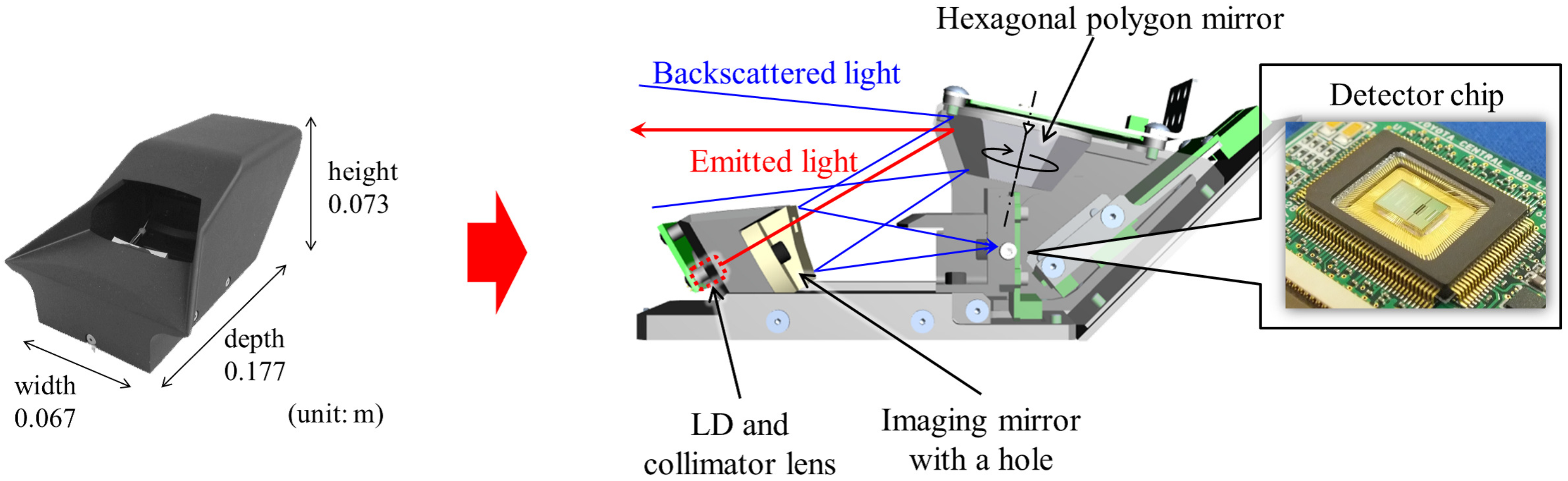
3.1. Small Imaging Sensor: SPAD LiDAR
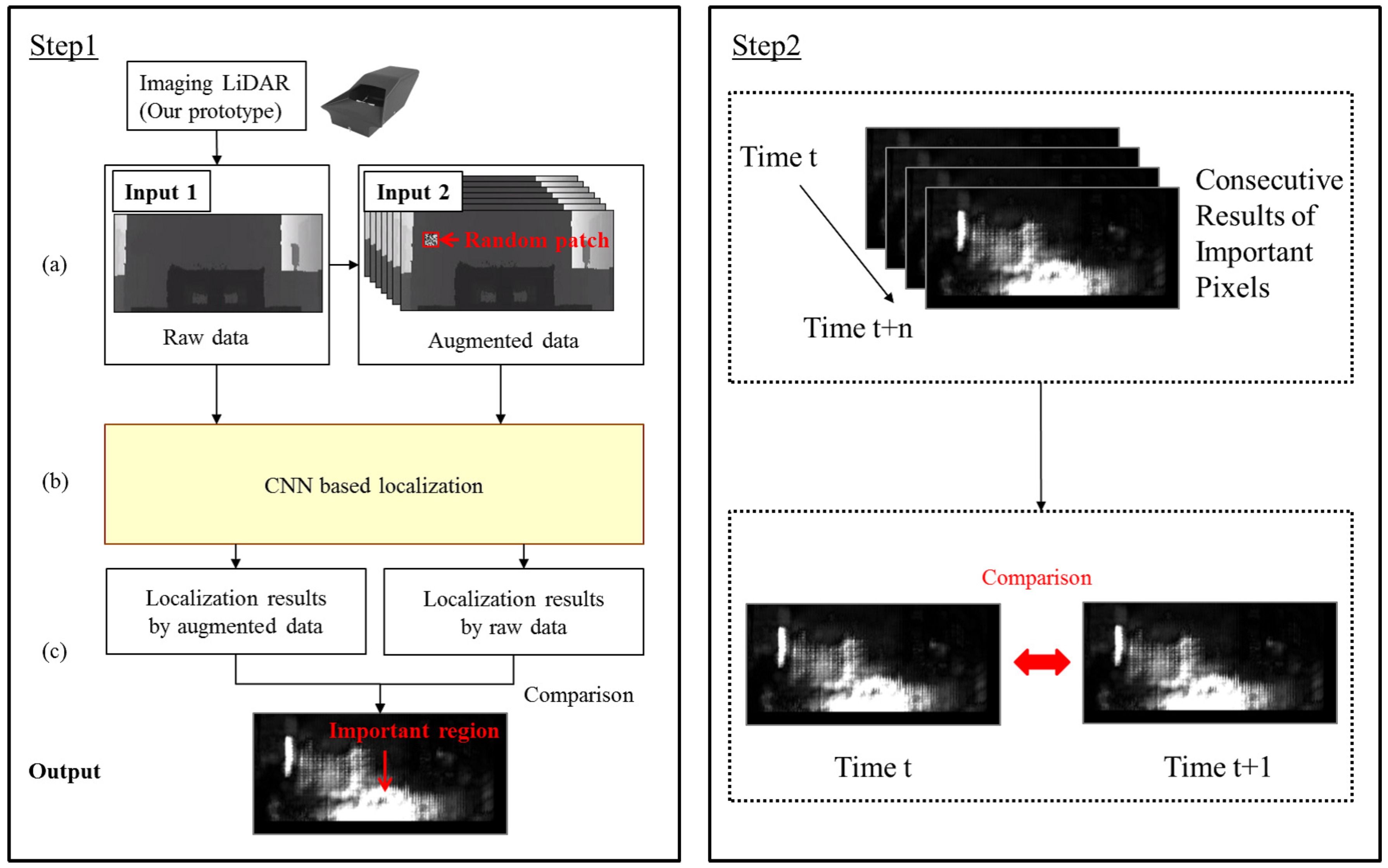
3.2. Quality Index Based on Important Pixels for CNN-Based Localization
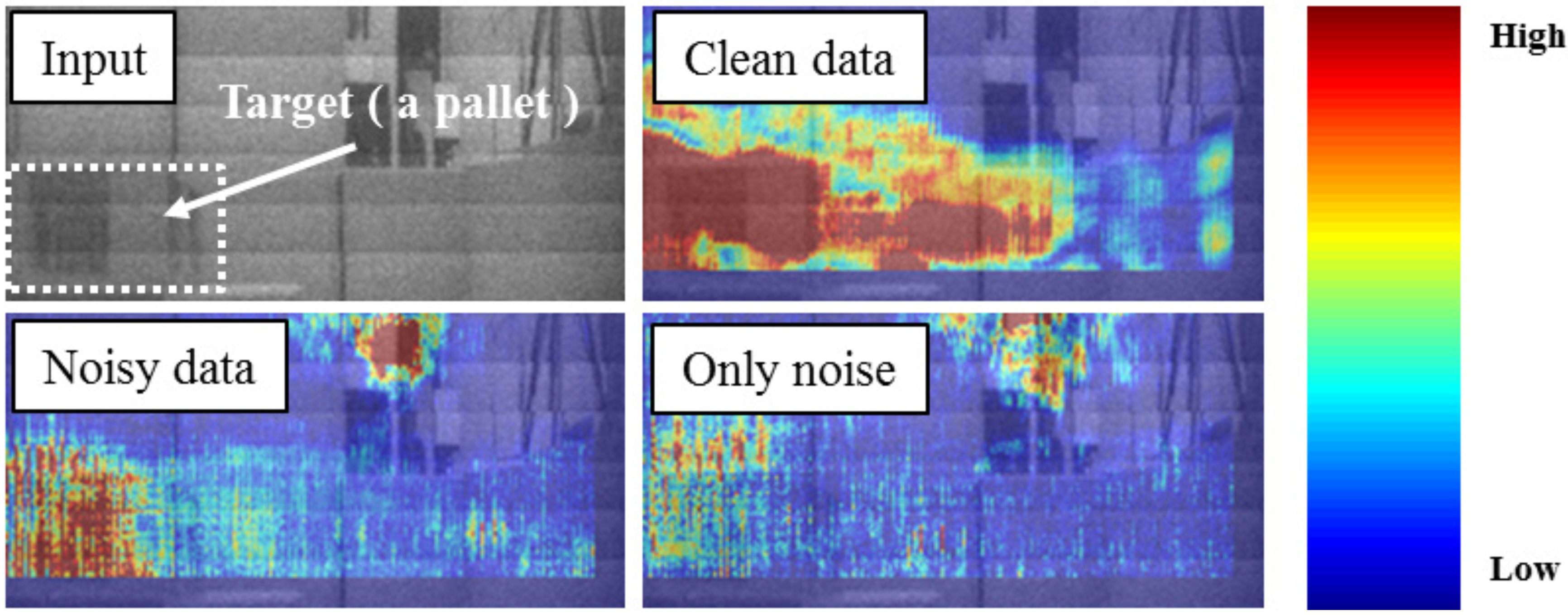
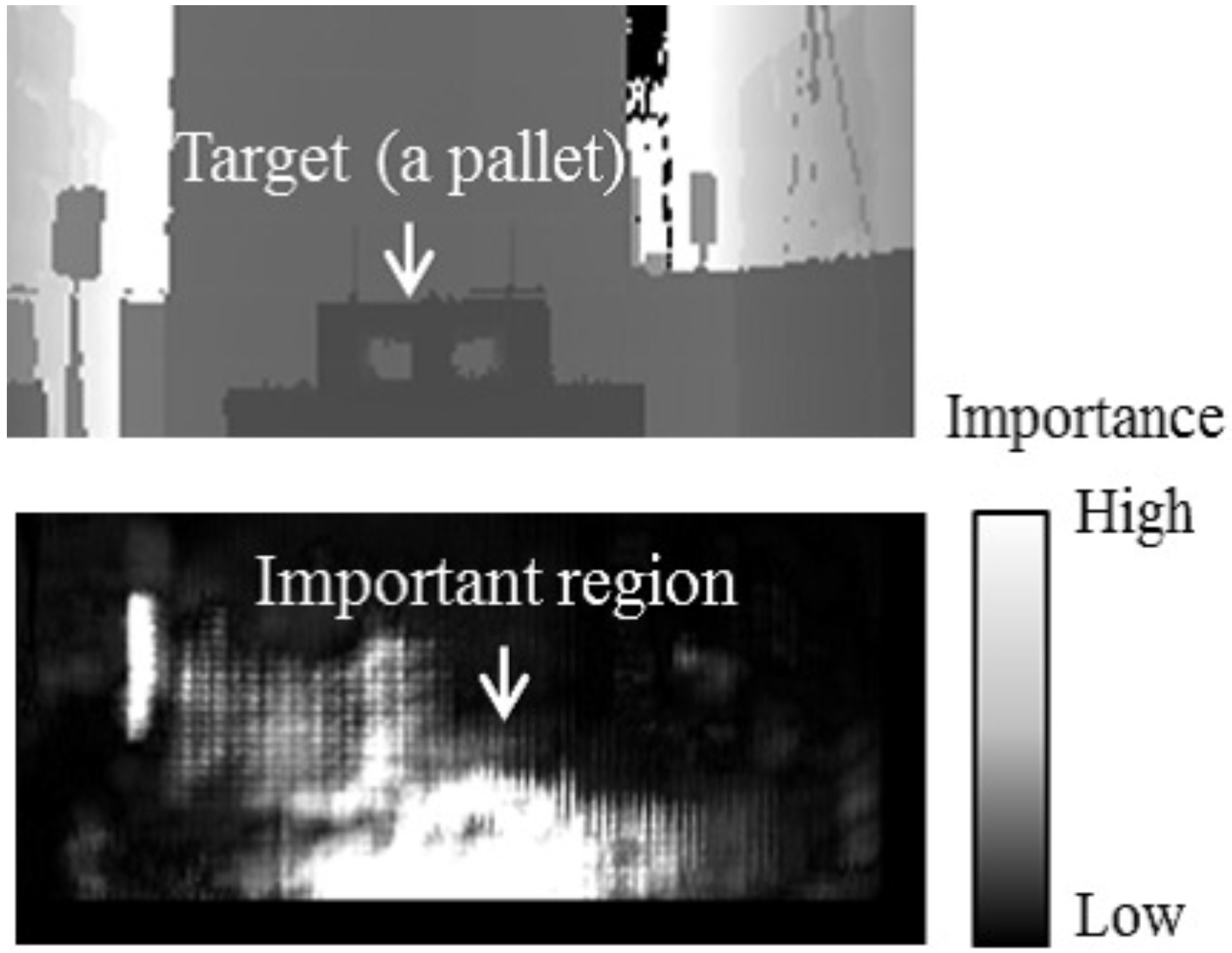
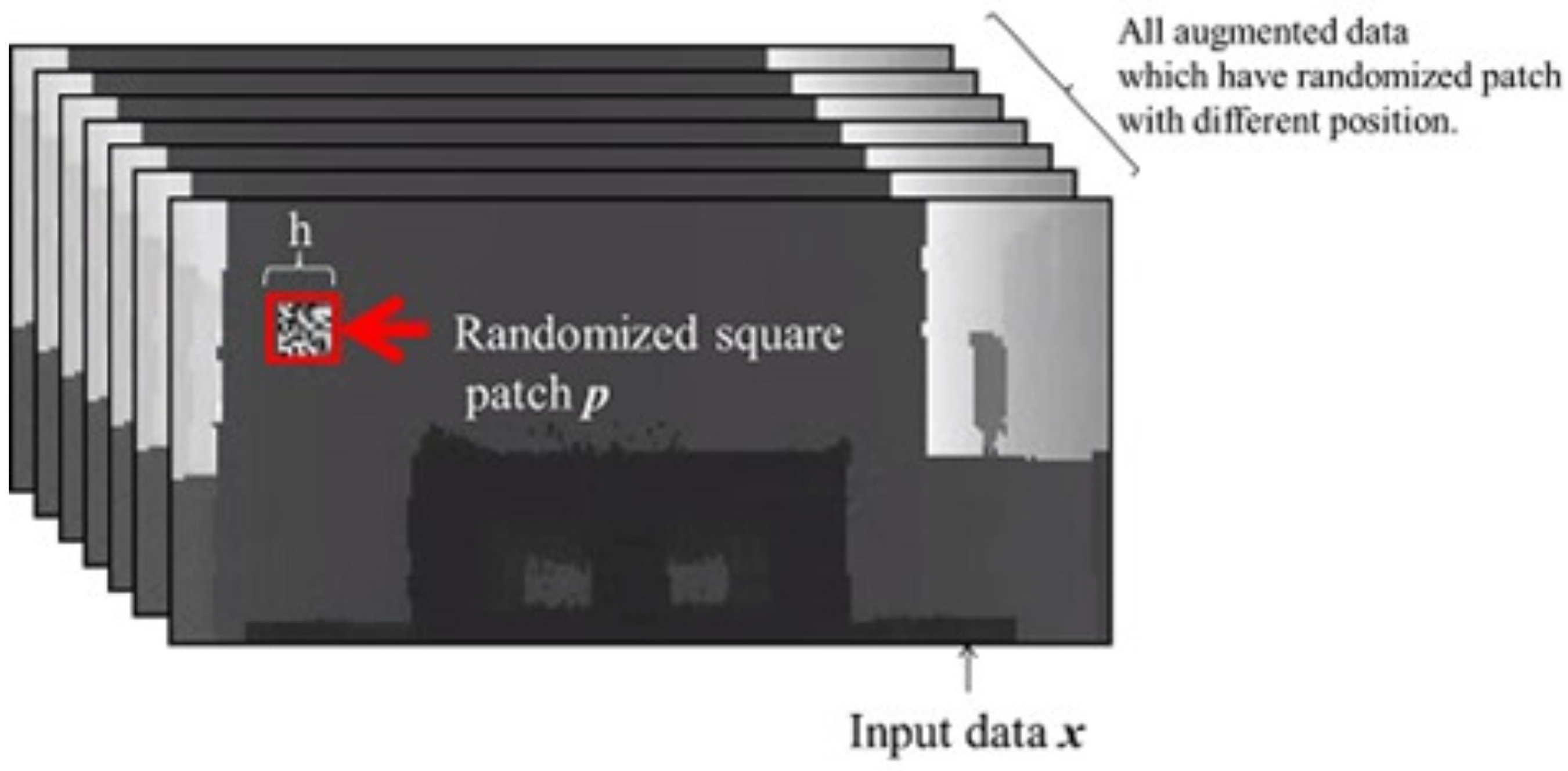
3.2.1. Step 1: Visualization of Important Pixels
3.2.2. Step 2: Quality Index
3.2.3. CNN-Based Localization
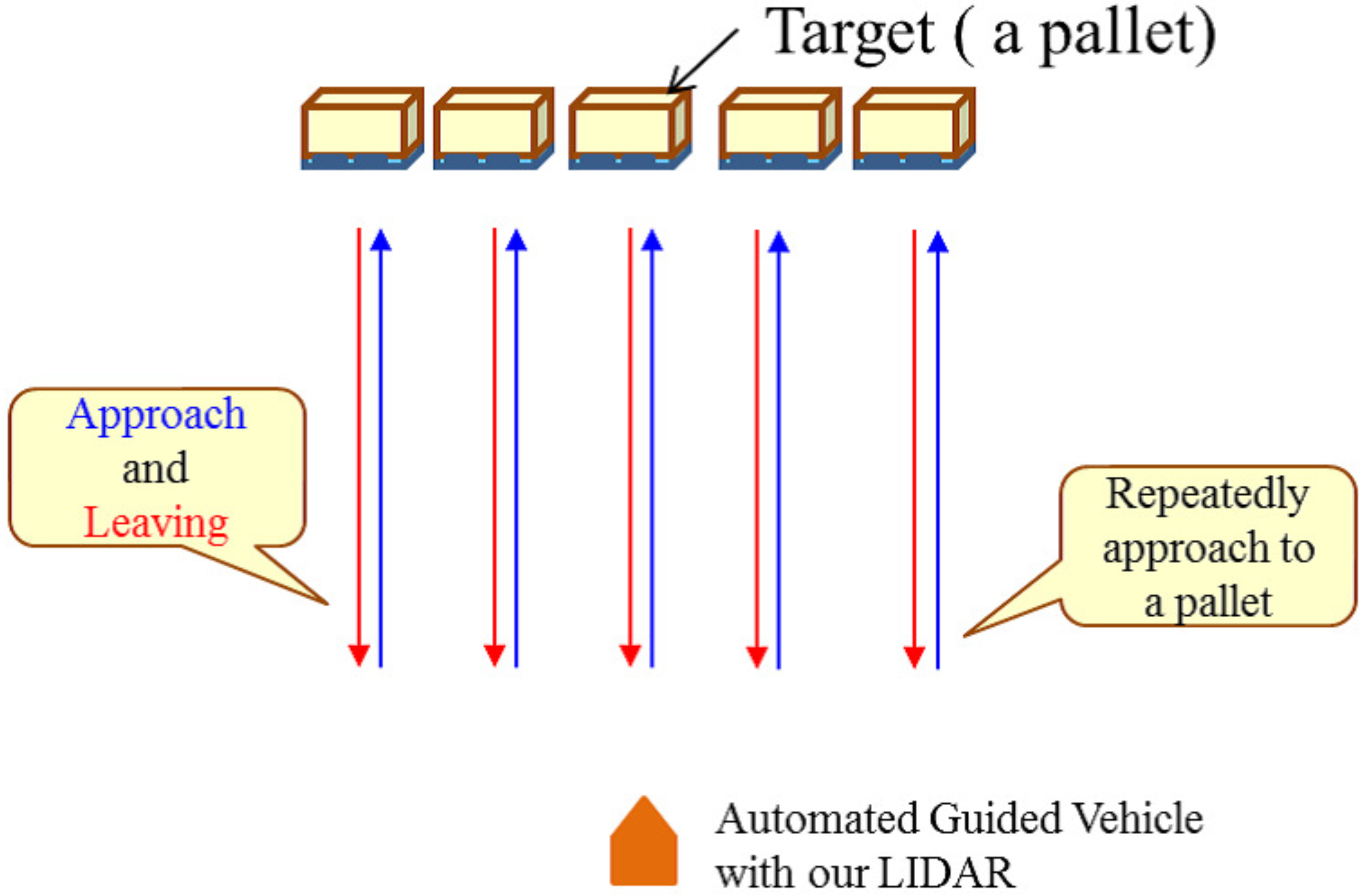
4. Experiments
- Reveal important pixels for CNN-based localization.
- The index reflects the quality of supervised data for CNN-based localization.
4.1. Results
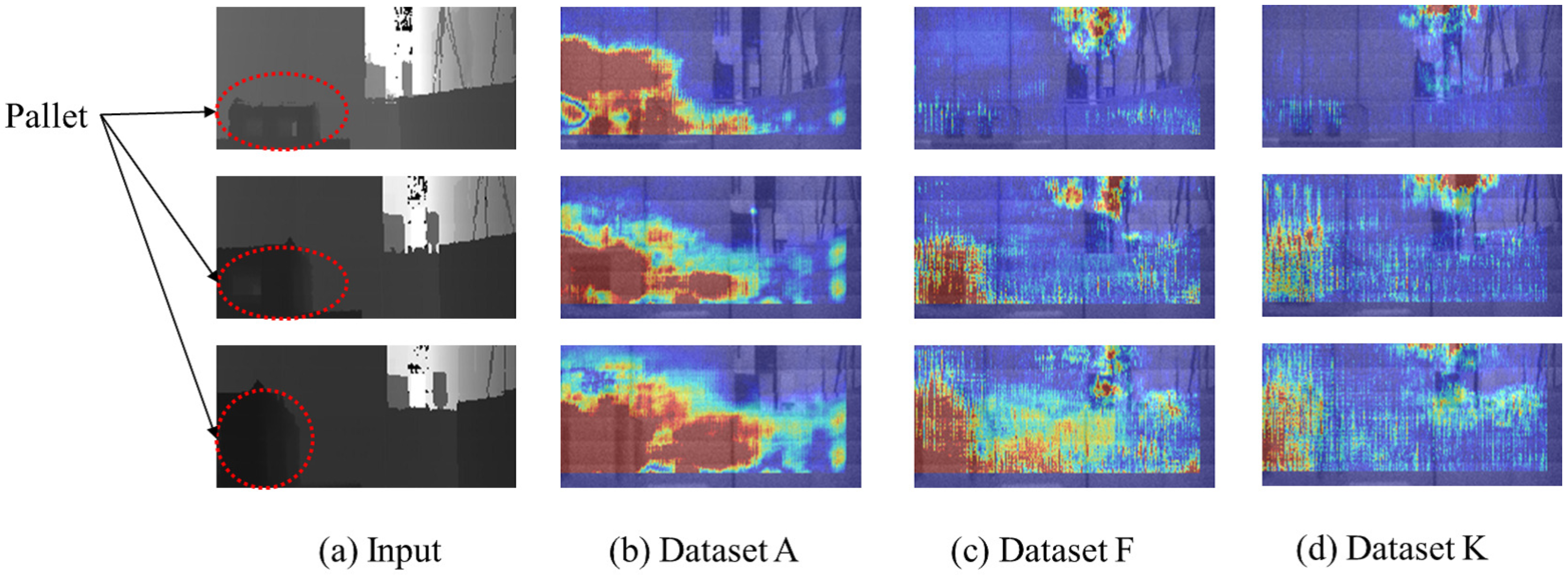
4.1.1. Important Pixels
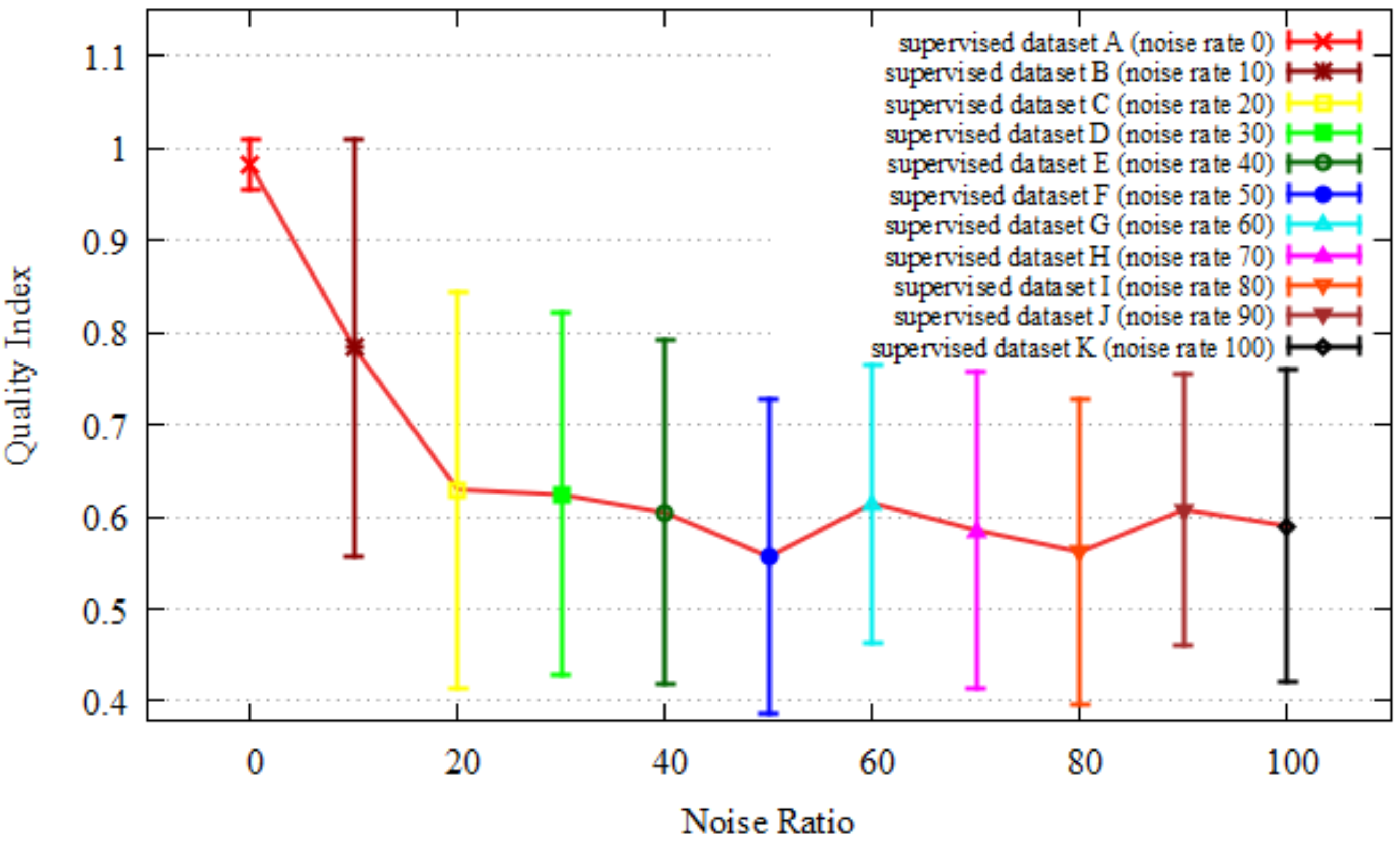
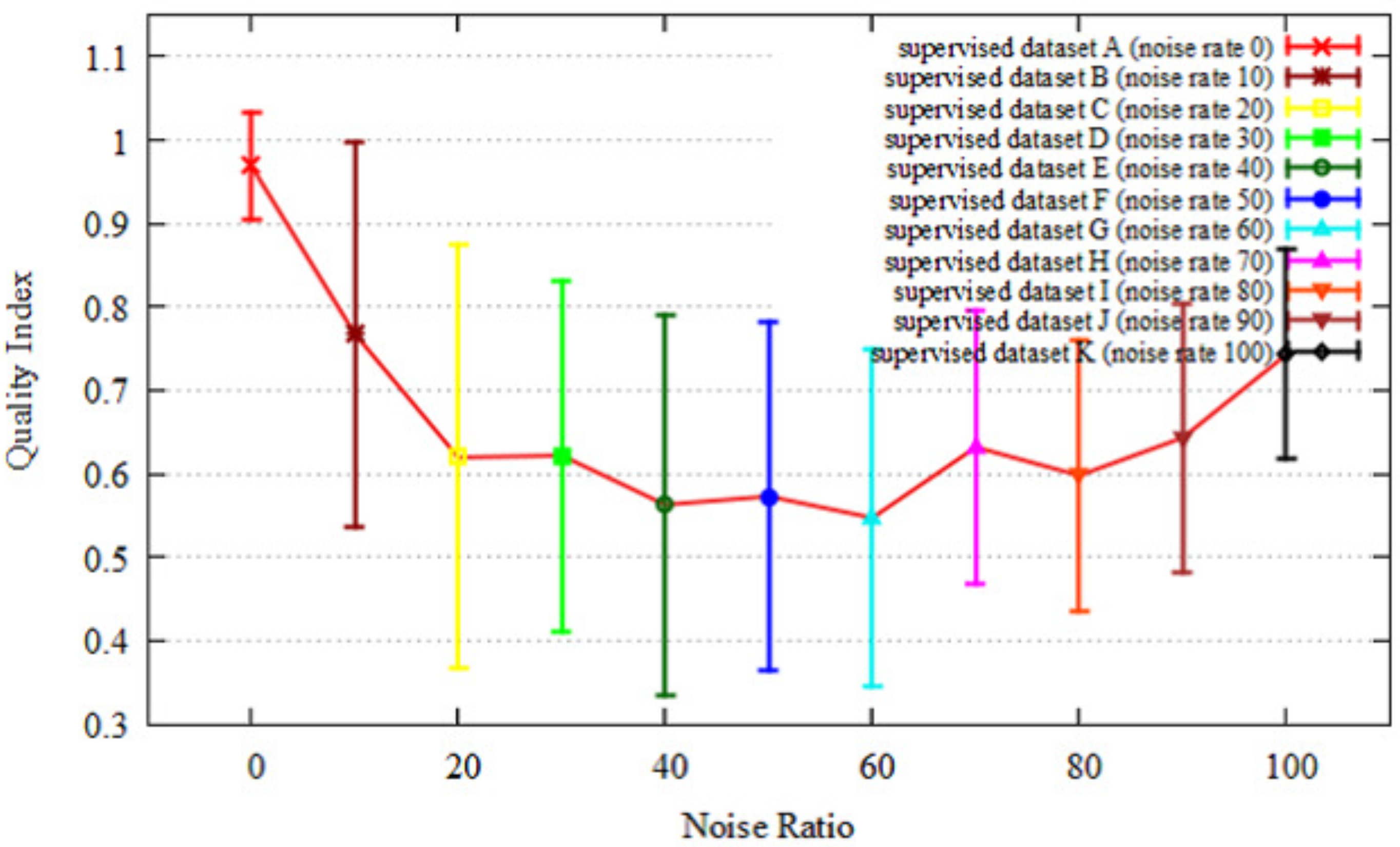
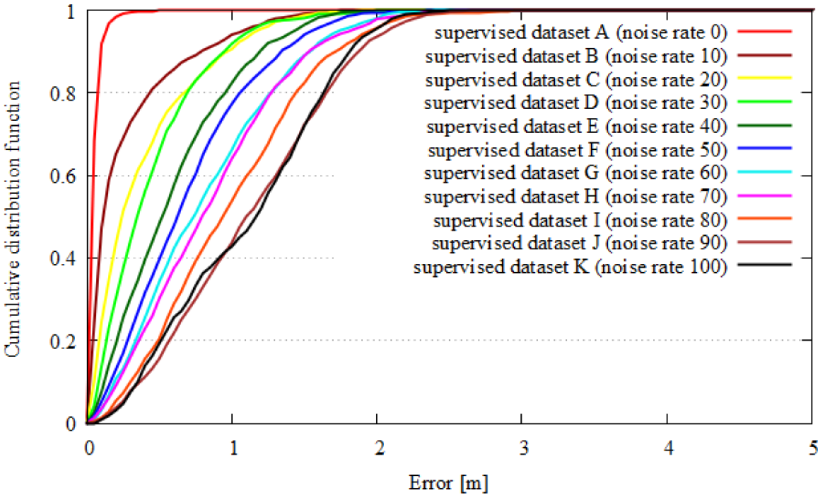
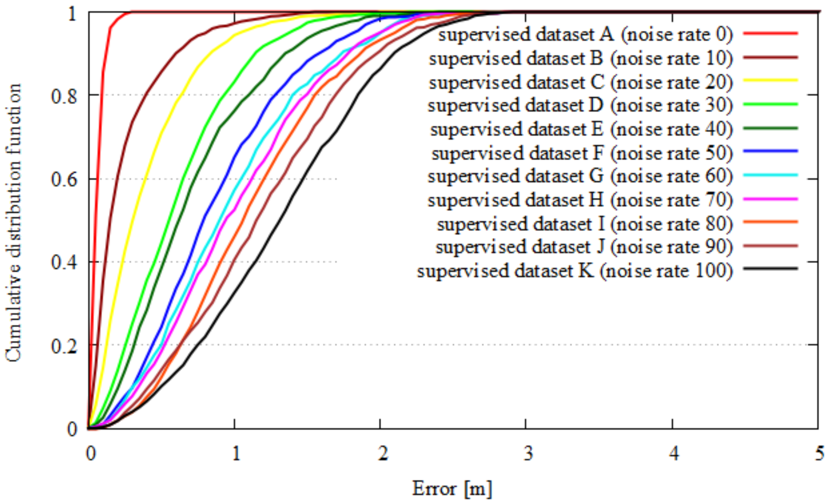
4.1.2. Quality Index and Localization
5. Conclusions
Author Contributions
Funding
Conflicts of Interest
References
- Velodyne 3D LiDAR. Available online: https://velodynelidar.com/products.html (accessed on 28 January 2019).
- SICK 3D LiDAR. Available online: https://www.sick.com/us/en/detection-and-ranging-solutions/3d-lidar-sensors/c/g282752 (accessed on 28 January 2019).
- Kendall, A.; Grimes, M.; Cipolla, R. PoseNet: A Convolutional Network for Real-Time 6-DOF Camera Relocalization. In Proceedings of the International Conference on Computer Vision (ICCV), Santiago, Chile, 13–16 December 2015. [Google Scholar]
- Arroyo, R.; Alcantarilla, P.F.; Bergasa, L.M.; Romera, E. Fusion and Binarization of CNN Features for Robust Topological Localization across Seasons. In Proceedings of the IEEE/RSJ International Conference on Intelligent Robots and Systems (IROS), Daejeon, Korea, 9–14 October 2016. [Google Scholar]
- Naseer, T.; Burgard, W. Deep Regression for Monocular Camera-based 6-DoF Global Localization in Outdoor Environments. In Proceedings of the IEEE/RSJ International Conference on Intelligent Robots and Systems (IROS), Vancouver, BC, Canada, 24–28 September 2017. [Google Scholar]
- Porzi, L.; Penate-Sanchez, A.; Ricci, E.; Moreno-Noguer, F. Depth-aware Convolutional Neural Networks for accurate 3D Pose Estimation in RGB-D Images. In Proceedings of the IEEE/RSJ International Conference on Intelligent Robots and Systems (IROS), Vancouver, BC, Canada, 24–28 September 2017. [Google Scholar]
- Yosinski, J.; Clune, J.; Nguyen, A.; Fuchs, T.; Lipson, H. Understanding Neural Networks through Deep Visualization. In Proceedings of the International Conference on Machine Learning Workshops (ICML), Lille, France, 6–11 July 2015. [Google Scholar]
- Van der Maaten, L.; Hinton, G. Visualizing data using t-SNE. J. Mach. Learn. Res. 2018, 9, 2579–2605. [Google Scholar]
- Springenberg, J.T.; Dosovitskiy, A.; Brox, T.; Riedmiller, M. Striving for Simplicity: The All Convolutional Net. In Proceedings of the International Conference on Learning Representations Workshops (ICLR Workshops), San Diego, CA, USA, 7–9 May 2015. [Google Scholar]
- Bojarski, M.; Choromanska, A.; Choromanski, K.; Firner, B.; Jackel, L.; Muller, U.; Zieba, K. VisualBackProp: Visualizing CNNs for autonomous driving. arXiv 2016, arXiv:1611.05418. [Google Scholar]
- Zhou, B.; Khosha, A.; Lapedriza, A.; Oliva, A.; Torralba, A. Object Detectors Emerge in Deep Scene CNNs. In Proceedings of the International Conference on Learning Representations (ICLR), San Diego, CA, USA, 7–9 May 2015. [Google Scholar]
- Zeiler, M.D.; Fergus, R. Visualizing and Understanding Convolutional Networks. In Proceedings of the European Conference on Computer Vision (ECCV), Zurich, Switzerland, 6–12 September 2014. [Google Scholar]
- Zintgraf, L.M.; Cohen, T.S.; Adel, T.A.; Welling, M. Visualizing Deep Neural Network Decisions: Prediction Difference Analysis. In Proceedings of the International Conference on Learning Representations Workshops (ICLR Workshops), Toulon, France, 24–26 April 2017. [Google Scholar]
- Niclass, C.; Soga, M.; Matsubara, H.; Kato, S.; Kagami, M. A 100-m-range 10-frame/s 340x96-pixel time-of-flight depth sensor in 0.18 μm CMOS. IEEE J. Solid-State Circuits 2013, 48, 559–572. [Google Scholar] [CrossRef]
- Ito, S.; Hiratsuka, S.; Ohta, M.; Matsubara, H.; Ogawa, M. SPAD DCNN: Localization with Small Imaging LIDAR and DCNN. In Proceedings of the IEEE/RSJ International Conference on Intelligent Robots and Systems (IROS), Vancouver, BC, Canada, 24–28 September 2017. [Google Scholar]
- Girshick, R. Fast-R-CNN. arXiv 2015, arXiv:1504.08083. [Google Scholar]
- Ren, S.; He, K.; Girshick, R.; Sun, J. Faster R-CNN: Toward Real-Time Object Detection with Region Proposal Networks. arXiv 2015, arXiv:1506.01497. [Google Scholar] [CrossRef] [PubMed]
- Quigley, M.; Conley, K.; Gerkey, B.; Conley, K.; Faust, J.; Foote, T.; Leibs, J.; Berger, E.; Wheeler, R.; Ng, A. ROS: An open-source Robot Operating System. In Proceedings of the IEEE International Conference on Robotics and AutomationWorkshops (ICRAWorkshops), Kobe, Japan, 12–17 May 2009. [Google Scholar]
- Abadi, M.; Barham, P.; Chen, J.; Chen, Z.; Davis, A.; Dean, J.; Devin, M.; Ghemawat, S.; Irving, G.; Isard, M.; et al. TensorFlow: A system for large-scale machine learning. In Proceedings of the USENIX Symposium on Operating Systems Design and Implementation (OSDI), Savannah, GA, USA, 2–4 November 2016. [Google Scholar]


| Specifications | |
|---|---|
| Pixel Resolution | 202 × 96 pixels |
| FOV | 55 × 9 degrees |
| Frame rate | 10 frames/s |
| Size | W 0.067 × H 0.073 × D 0.177 m |
| Range | 70 m |
| Wavelength | 905 nm |
| Frequency | 133 kHz |
| Peak power | 45 W |
| TOF measurement | Pulse type |
| Laser | Class 1 laser |
| Distance resolution | 0.035 m (short-range mode), 0.070 m (long-range mode) |
| All Dataset | |
|---|---|
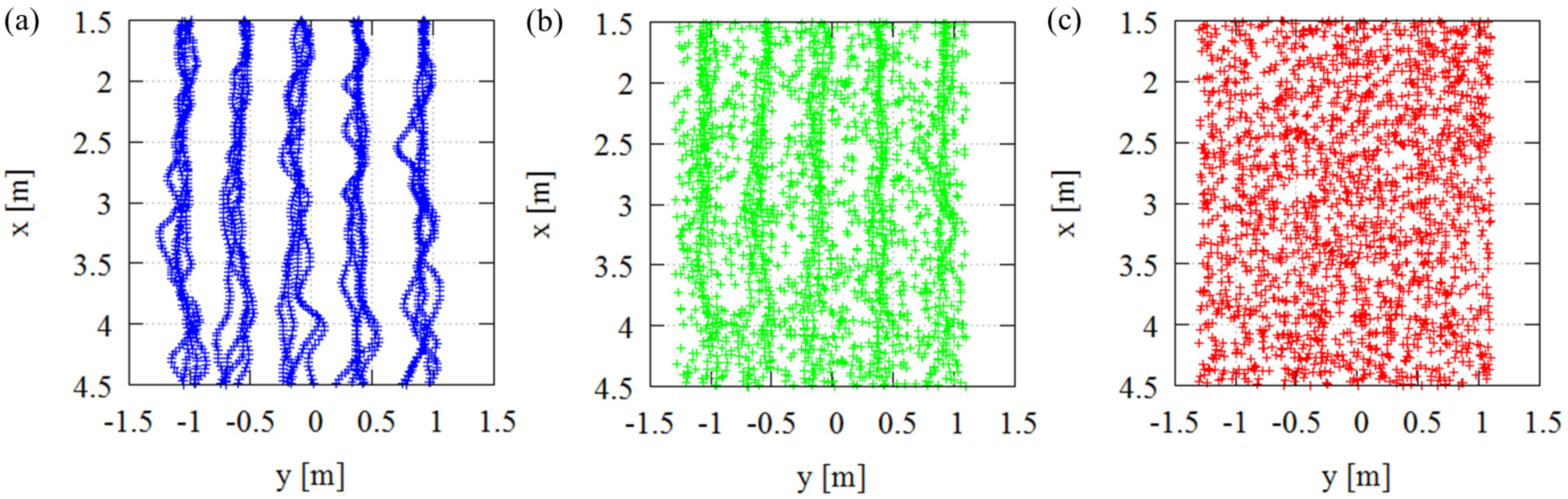
| Dataset A | Original motion capture dataset |
| Dataset B | 10% of data were replaced with noise |
| Dataset C | 20% of data were replaced with noise |
| Dataset D | 30% of data were replaced with noise |
| Dataset E | 40% of data were replaced with noise |
| Dataset F | 50% of data were replaced with noise |
| Dataset G | 60% of data were replaced with noise |
| Dataset H | 70% of data were replaced with noise |
| Dataset I | 80% of data were replaced with noise |
| Dataset J | 90% of data were replaced with noise |
| Dataset K | All of data were replaced with noise |
© 2019 by the authors. Licensee MDPI, Basel, Switzerland. This article is an open access article distributed under the terms and conditions of the Creative Commons Attribution (CC BY) license (http://creativecommons.org/licenses/by/4.0/).
Share and Cite
Ito, S.; Soga, M.; Hiratsuka, S.; Matsubara, H.; Ogawa, M. Quality Index of Supervised Data for Convolutional Neural Network-Based Localization. Appl. Sci. 2019, 9, 1983. https://doi.org/10.3390/app9101983
Ito S, Soga M, Hiratsuka S, Matsubara H, Ogawa M. Quality Index of Supervised Data for Convolutional Neural Network-Based Localization. Applied Sciences. 2019; 9(10):1983. https://doi.org/10.3390/app9101983
Chicago/Turabian StyleIto, Seigo, Mineki Soga, Shigeyoshi Hiratsuka, Hiroyuki Matsubara, and Masaru Ogawa. 2019. "Quality Index of Supervised Data for Convolutional Neural Network-Based Localization" Applied Sciences 9, no. 10: 1983. https://doi.org/10.3390/app9101983
APA StyleIto, S., Soga, M., Hiratsuka, S., Matsubara, H., & Ogawa, M. (2019). Quality Index of Supervised Data for Convolutional Neural Network-Based Localization. Applied Sciences, 9(10), 1983. https://doi.org/10.3390/app9101983