Implementation and Experimental Verification of Flow Rate Control Based on Differential Flatness in a Tilting-Ladle-Type Automatic Pouring Machine

Abstract

In this paper, we study an advanced pouring control system using a tilting-ladle-type automatic pouring machine. In such a machine, it is difficult to precisely pour the molten metal into the pouring basin of the mold, as the outflow from the ladle can be indirectly controlled by controlling its tilt. Therefore, model-based pouring control systems have been developed as a part of conventional studies to solve this problem. In the results of a recent study, the efficacy of a pouring flow rate control system based on differential flatness has been verified, by performing a simulation. In this study, we apply the flow rate control system based on differential flatness to a tilting-ladle-type automatic pouring machine, using experiments to verify the efficacy of the flow rate control system in suppressing any disturbances. In these experiments, the tracking performance using the developed flow rate control system was better than the performance obtained using a conventional feed-forward-type flow rate control system.

1. Introduction

In the casting industry, the pouring process creates a dangerous working environment, involving high-temperature molten metal. Therefore, automatic pouring systems have been developed and applied to keep workers away from the pouring site [1,2]. Recently, a tilting-ladle-type automatic pouring system has been developed, which is simple to construct and which allows the molten metal in the ladle to be easily changed [3]. An automatic pouring machine must be able to precisely and quickly pour molten metal into a mold, to ensure the quality of the cast product and to ensure safety in the working environment. However, it is difficult to precisely pour molten metal into the pouring basin of a mold, as the outflow from the ladle can be indirectly controlled by controlling its tilt [4,5,6,7].

Pouring control systems which can be used to precisely pour a liquid by tilting the liquid container have been proposed in previous studies. A mathematical model that represents the pouring process using an automatic pouring system has been derived, and a feed-forward flow rate control system, based on the inverse model, has been developed by the present authors [8]. Furthermore, feed-forward flow rate control has been applied to control the liquid level in the tundish of a strip-caster [9]. The supervisory control of an automatic pouring system with a fan-shaped ladle was proposed, in order to perform multiple tasks: To ensure that the liquid in the pouring basin was maintained at a constant level; that the total quantity of the liquid that was poured into the mold was achieved precisely at the target quantity; and that sloshing of the liquid in the ladle was suppressed [10]; in this approach, flow rate control was achieved using feed-forward control based on the inverse pouring model. The parameters of the inverse pouring model in the feed-forward control have been adaptively tuned, using the on-line model parameters identification method [11]. Additionally, the motion of the liquid container was optimized using a computer fluid dynamics simulation based on the Navier-Stokes model [12,13]. Recently, the model-based pouring control system was applied to a pouring robot, which was constructed with a parallel mechanism [14]. Other recent pouring control approaches have noted that the falling position and flow rate of the outflow liquid from the ladle can be directly manipulated from a remote location [15]. In the previously-described approaches, various pouring control systems have been proposed with model-based designs, and feed-forward control approaches are employed in most of them.

As for pouring control using model-free approaches, various feedback control systems have been proposed to ensure that the liquid volume in the target container can be achieved at the target volume, using a vision system [16,17]. More recently, the liquid poured from an unknown container, which has a simple and symmetric shape, has been controlled by estimating the geometry of the container shape, using the model learning approach [18,19]. These approaches are robust with respect to the shape of the source container, and specialize in ensuring that the total liquid volume poured from the source container is achieved precisely at the target volume. However, flow rate control is very important for designing a high-precision automatic pouring machine in the casting field, as the flow rate influences the pouring conditions, including the falling position of the outflow liquid, the liquid level in the target container, and the total outflow.

Some pouring control systems have been proposed based on the model-based feedback approach. A real-time flow rate estimation system was developed, using an extended Kalman filter based on the pouring model [20]. Additionally, an un-scented Kalman filter was applied to realize real-time flow rate estimation for a ladle with a complicated shape [21]. To construct a flow rate feedback control system, the present authors developed a flow rate control based on differential flatness [22]. A cascade control system, exhibiting flow rate feedback control and liquid level control in the pouring basin, was proposed in a recent study [23]. In previous studies, the efficacy of flow rate feedback control was verified using only simulation. To the best of our knowledge, the implementation and experimental verification of flow rate control systems using the feedback approach have not been previously studied.

Therefore, in this study, pouring flow rate control based on differential flatness is implemented for a tilting-ladle-type automatic pouring machine, and the efficacy of flow rate control is verified through experiments. During the implementation of the flow rate control, an extended Kalman filter based on the pouring model is applied for estimating the state variables of the automatic pouring machine, and these variables are used to achieve flow rate control. In the control design, based on differential flatness, a two degree-of-freedom control system can be constructed for a control object exhibiting non-linear characteristics. This study addresses the problem in the implementation of flow rate feedback control [22] that the load cell data is perturbed by the vertical motion of ladle. In the experiments, the flow rate control system developed in this study is compared with a conventional feed-forward-type pouring flow rate control system.

The remainder of this study is organized as follows. The second section provides an overview of the tilting-ladle-type automatic pouring machine. The modeling of the tilting-ladle-type automatic pouring machine is presented in the third section. Further, the fourth section presents the design of the pouring flow rate control based on differential flatness. Then, the implementation of the developed system is described in the fifth section. The efficacy of the system is verified through experiments, as described in the sixth section. Finally, we summarize our observations.

2. Tilting-Ladle-Type Automatic Pouring Machine

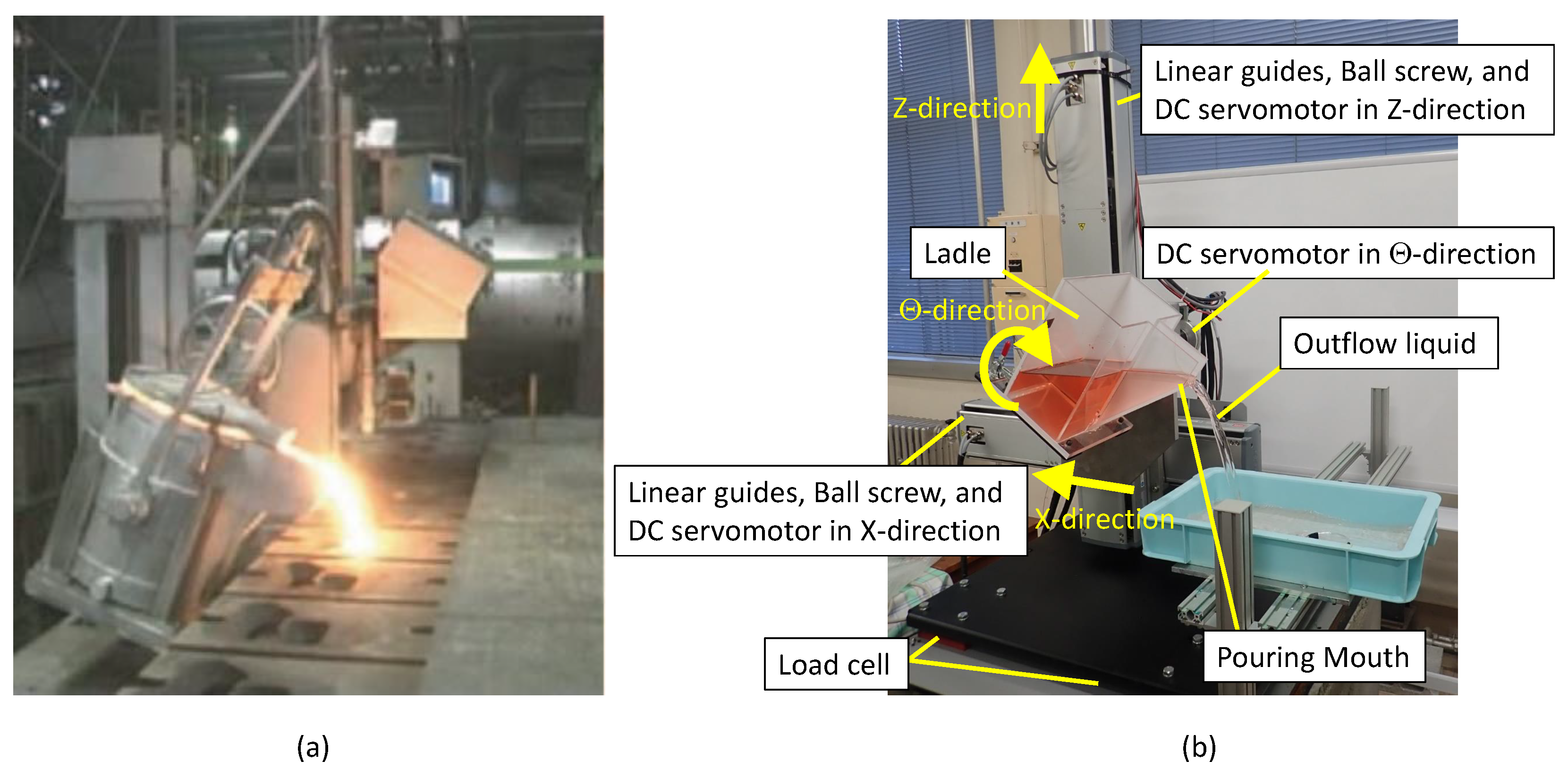
A tilting-ladle-type automatic pouring machine that is actually applied in a casting plant is depicted in Figure 1a. The tilting-ladle-type automatic pouring machine that has been developed in the present laboratory of the authors is depicted in Figure 1b. The developed pouring machine is smaller than the one in the casting plant; however, they perform similar functions with respect to their drive and sensor systems. The ladles in both the pouring machines can be moved in the front–back, up–down, and rotational directions, for three degrees-of-freedom of motion. In this study, the front–back, up–down, and rotational directions are denoted as the X-, Z-, and $\Theta$-directions, respectively. Further, each drive system in the X- and Z-directions is comprised of linear guides, a ball screw, and a servomotor. The drive system in the $\Theta$-direction is comprised of a gear reducer and servomotor. The positions of the ladle in the X- and Z-directions and the angle of the ladle in $\Theta$-direction can be detected, using the rotary encoders in the servomotor systems. The specifications of the drive systems in the pouring machine developed in our laboratory are presented in

Table 1. Specifications of drive systems in the tilting-ladle-type automatic pouring machine developed by the authors.

	X-Direction	Z-Direction	$\mathbf{\Theta }$-Direction
Type of motor	Brushless DC motor	Brushless DC motor	Brushless DC motor
Control mode in servo amplifier	Velocity mode	Velocity mode	Velocity mode
Motion range	0–0.3 m	0–0.4 m	0–70 deg
Maximum torque of motor	1.22 Nm	1.22 Nm	11.5 Nm
Pitch of ball screw	0.02 m	0.02 m	-
Maximum velocity of motor	0.77 m/s	0.38 m/s	371 deg/s

. Additionally, the weight of the liquid in the ladle can be measured, using the load cell installed in the base of the machine. Therefore, the total weight of the outflow liquid from the ladle can be obtained, based on the difference between the initial and the current weights of the liquid in the ladle. The combined error of the load cell is 0.1 kg.

The command signals to the drive systems are calculated by a PC-based controller, in which the CPU is an Intel Core i7-4790 (Intel Corporation, Santa Clara, CA, USA) and the memory is 8 GB DDR3-1600 (Corsair Corporation, Fermon, CA, USA). The sampling period in the control system is 0.02 s. The signals between the controller and the drive systems are transferred by a controller area network (CAN) communication method, and the signal from the load cell to the controller is transferred by a serial communication method for reducing noise in the communication.

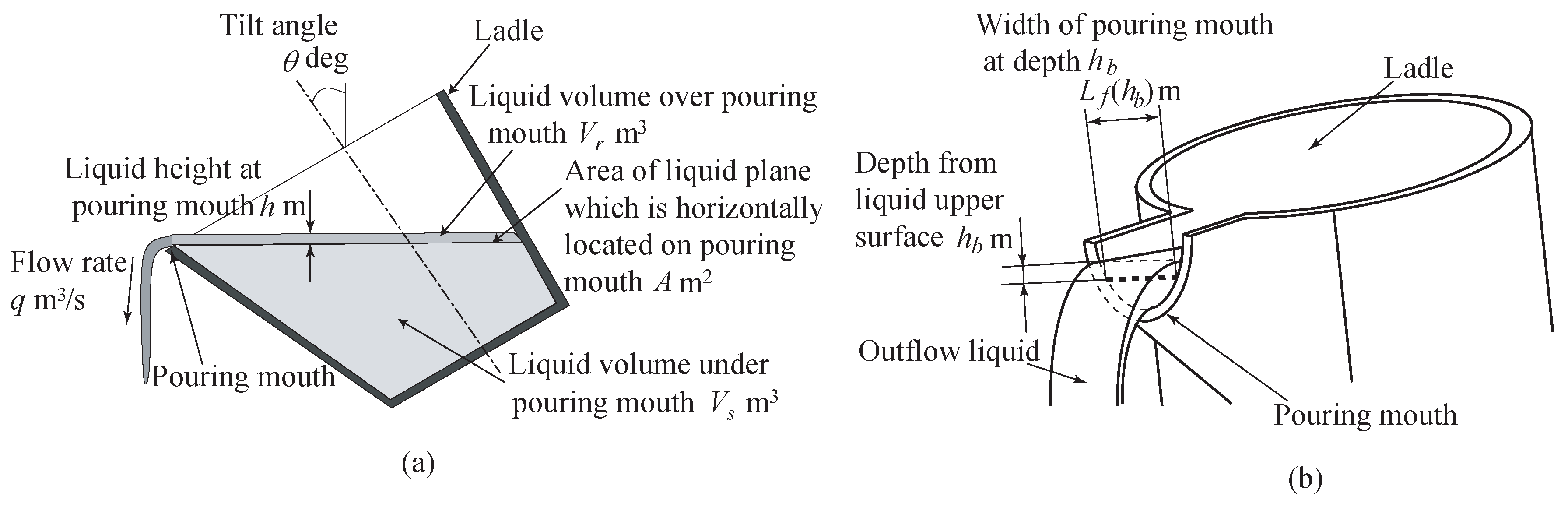
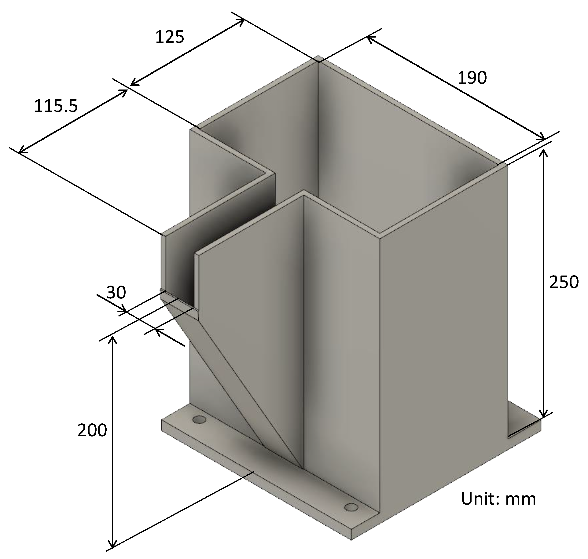
Figure 2 depicts the shape of the ladle used in this study. For safety reasons, water was considered to be the target liquid and the ladle was manufactured using acrylic plates, as depicted in Figure 1b.

3. Modeling of the Tilting-Ladle-Type Automatic Pouring Machine

The tilting-ladle-type automatic pouring machine is comprised of drive systems for the X-, Z-, and $\Theta$-axes, a pouring process, and a load cell; as presented in the previous section. The signal diagram of the pouring machine is depicted in Figure 3. An input signal is applied to the servomotor of the $\Theta$-axis for tilting the ladle, causing the liquid in the ladle to be poured into the mold. Further, the weight of the outflow liquid is measured using the load cell. The input signals are also applied to the servomotors of the X- and Z-axes. Here, the acceleration in the Z-direction is convoluted to the response of the load cell, because the response of the load cell can be affected by the motion of the ladle in the Z-direction.

3.1. Motor Model on the $\Theta$-Axis

As the velocity control mode is applied in the servo amplifier of the $\Theta$-axis, the motor model $P_T$ in Figure 3 used for tilting the ladle can be described simply by the linear first-order system:

$$\dot{\omega }\left(t\right)=-\frac{1}{T_t}\omega \left(t\right)+\frac{K_t}{T_t}{u}_t\left(t\right)$$

(1)

where $\omega$ deg/s denotes the angular velocity of the tilting ladle, $u_t$ denotes the input signal applied to the motor, $T_t$ s denotes the time constant, and $K_t$ deg/s denotes the gain. The tilt angle, $\theta$ (in deg), is given as

$$\dot{\theta }\left(t\right)=\omega \left(t\right),$$

(2)

and can be measured using the rotary encoder fitted to the servomotor.

3.2. Motor Models on the X- and Z-Axes

As the velocity control mode is applied in the servo amplifiers of the X- and Z-axes, the motor models $P_X$ and $P_Z$ depicted in Figure 3 for transferring the ladle on the X- and Z-axes, respectively, can be described simply by a linear first-order system:

$${\dot{v}}_i\left(t\right)=-\frac{1}{T_i}{v}_i\left(t\right)+\frac{K_i}{T_i}{u}_i\left(t\right),(i=x,z),$$

(3)

where $v_i$ m/s denotes the velocity of the transferring ladle on each axis, $u_i$ denotes the input signal applied to each motor, $T_i$ s denotes the time constant, and $K_i$ m/s denotes the gain. The subscript i represents the drive direction. The positions $x_x$ and $x_z$ m of the ladle are given as

$$\dot{x_i}\left(t\right)=v_i\left(t\right),(i=x,z),$$

(4)

and can be measured using the rotary encoder fitted to each servomotor.

3.3. Pouring Process Model

The model $P_F$ in Figure 3 represents the pouring process from the angular velocity of the tilting ladle to the flow rate of the outflow liquid, as described in detail in [8,22]. A cross-section of the pouring process is depicted in Figure 4a, where $\theta$ denotes the tilt angle of the ladle, $V_s\left(\theta \right)$ m³ denotes the liquid volume under the pouring mouth, and $A\left(\theta \right)$ m² denotes the area of the liquid plane, which is horizontal to the pouring mouth. The volume $V_s\left(\theta \right)$ and area $A\left(\theta \right)$ are dependent on the tilt angle $\theta$. $V_r$ m³ denotes the volume over the area $A\left(\theta \right)$, and h m denotes the liquid height at the pouring mouth. When the liquid level is above the lip of the pouring mouth, it flows out of the ladle at the flow rate q m³/s. The pouring process model, $P_F$, can be described by the mass balance of the liquid in the ladle and Bernoulli’s theorem, as

$$\dot{h}\left(t\right)=-\frac{q\left(h\right(t\left)\right)}{A\left(\theta \right(t\left)\right)}-\frac{1}{A\left(\theta \right(t\left)\right)}\left(\frac{\partial A\left(\theta \right(t\left)\right)}{\partial \theta \left(t\right)}h\left(t\right)+\frac{\partial V_s\left(\theta \left(t\right)\right)}{\partial \theta \left(t\right)}\right)\omega \left(t\right),$$

(5)

$$q\left(h\left(t\right)\right)=c{\int }_0^{h\left(t\right)}{L}_f\left(h_b\right)\sqrt{2g{h}_b}d{h}_b,$$

(6)

where $h_b$ m denotes the depth from the upper surface of the liquid, as shown in Figure 4b, and $L_f\left(h_b\right)$ m is the width of the pouring mouth at the depth $h_b$. In addition, c is the flow rate coefficient and g m/s² is the acceleration of gravity.

The actual weight, $w_o$ kg, of the liquid flowing out of the ladle is represented as

$${\dot{w}}_o\left(t\right)=\rho q\left(h\left(t\right)\right),$$

(7)

where $\rho$ kg/m³ denotes the density of the liquid in the ladle.

3.4. Load Cell Model

The load cell measures not only the weight of the liquid flowing out of the ladle, but also the motion of the part transferred along the Z-axis, as depicted in Figure 3. Here, the data from the load cell are unaffected by the tilting motion of the ladle, because the rotational axis is located through the center of gravity of the ladle. The output of the load cell is adjusted to the gravity environment on the earth, and does not consider the vertical motion of the measured object. Therefore, it is required to compensate for the weight of the part transferred along the Z-axis by the relation:

$$w_z^{\prime }g=w_z{a}_z,$$

(8)

where $w_z$ kg and $a_z$ m/s² denote the weight and acceleration of the part moving along the Z-axis, respectively. The acceleration, $a_z$, can be derived as $a_z={\dot{v}}_z$ from Equation (3), and $w_z^{\prime }$ kg denotes the weight which appears in the load cell data during the vertical motion of the ladle. Moreover, we assume that the vibration of the load cell is small because the natural frequency of the load cell is much higher than the dynamics of the pouring motion. Therefore, the dynamics, $P_L$, of the load cell are modeled simply by a linear first-order system:

$${\dot{w}}_l\left(t\right)=-\frac{1}{T_l}{w}_l\left(t\right)+\frac{1}{T_l}\left(w_o\left(t\right)+\frac{w_z}{g}{a}_z\left(t\right)\right),$$

(9)

where $w_l$ kg denotes the weight of the outflow liquid measured by the load cell and $T_l$ s denotes the time constant representing the response of the load cell.

4. Design of the Pouring Flow Rate Control Based on Differential Flatness

The pouring flow rate control can be designed based on differential flatness, which has been described in detail in [22,24]. The controller design is applied to the plant model presented in Equations (1), (2), (5) and (6). Further, the response of the drive system is considerably faster than that of the pouring process, because the time constant is approximately one-hundredth of that in pouring process. Therefore, the dynamics of the motor $P_M$ of the $\Theta$-axis can be neglected, to simplify the plant model. Furthermore, as depicted in [22], there is a considerable requirement to ensure the tracking performance of the flow rate in an automatic pouring machine with precision pouring; however, the tracking performance of the tilt angle of the ladle is not necessary. The liquid height is considerably related to the flow rate, as depicted in Equation (6). Therefore, we focus on the dynamic model of the liquid height, h, for designing the flow rate control. Consequently, the simplified plant model for the design of the flow rate control is represented as a single input and single output (SISO)-nonlinear first-order dynamic system:

$$\dot{h}\left(t\right)=-\frac{1}{A\left(\theta \right)}q\left(h\left(t\right)\right)-\frac{1}{A\left(\theta \right)}\left(\frac{\partial V_s\left(\theta \right)}{\partial \theta }+\frac{\partial A\left(\theta \right)}{\partial \theta }h\left(t\right)\right)K_t{u}_t\left(t\right).$$

(10)

The flat output F to Equation (10) is given as follows:

$$F=h\left(t\right).$$

(11)

Additionally, the input $u_t$ can be derived by the flat output, as follows:

$$u_t\left(t\right)=-\frac{A\left(\theta \right)\dot{F}\left(t\right)+q\left(F\left(t\right)\right)}{K_t\left(\frac{\partial V_s\left(\theta \right)}{\partial \theta }+\frac{\partial A\left(\theta \right)}{\partial \theta }F\left(t\right)\right)}.$$

(12)

Further, the new input $\nu$ is introduced by the following transformation:

$$u_t\left(t\right)=-\frac{A\left(\theta \right)\nu \left(t\right)+q\left(F\right(t\left)\right)}{K_t\left(\frac{\partial V_s\left(\theta \right)}{\partial \theta }+\frac{\partial A\left(\theta \right)}{\partial \theta }F\left(t\right)\right)}.$$

(13)

Subsequently, the pouring process, using the new input $\nu$, can be described as a single integrator:

$$\dot{F}=\nu .$$

(14)

Based on Equation (14), the linear feedback tracking controller can be set up using the proportional–integral–derivative (PID) scheme:

$$\nu \left(t\right)={\dot{F}}^{\ast }-{\beta }_1(F-F^{\ast })-{\beta }_0\int (F-F^{\ast })dt,$$

(15)

which includes the reference trajectory $F^{\ast }\left(t\right)=h^{\ast }\left(t\right)$ of the liquid height and the control parameters ${\beta }_0$ and ${\beta }_1$. Then, the dynamics of the tracking error e, which is given as $\dot{e}=F-F^{\ast }$, can be derived as

$$\ddot{e}+{\beta }_1\dot{e}+{\beta }_{0}e=0,$$

(16)

using the characteristic polynomial

$$\phi \left(s\right)=s^2+{\beta }_{1}s+{\beta }_0.$$

(17)

The coefficients ${\beta }_0$ and ${\beta }_1$ are arranged for satisfying the exponential stability of the closed-loop system as follows:

$${\beta }_0={\omega }_n^2,{\beta }_1=2\zeta {\omega }_n,(\zeta \ge 1,{\omega }_n>0),$$

(18)

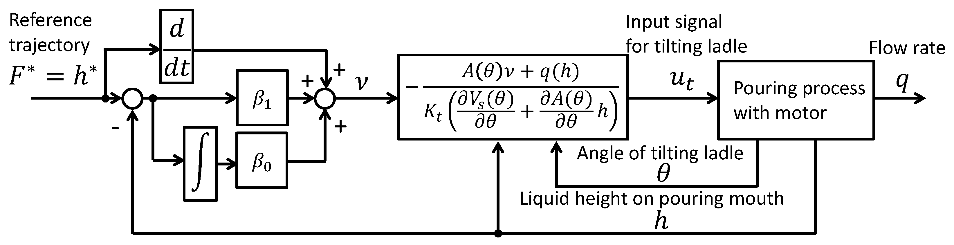
where $\zeta$ is the damping ratio and ${\omega }_n$ rad/s is the natural angular frequency in the general form of a second-order system. To achieve exponential stability of the error e, the coefficients are given as $\zeta \ge 1$ and ${\omega }_n>0$. The signal diagram of the flow rate control based on differential flatness is depicted in Figure 5.

The control input, $u_t$, can be decomposed into a feed-forward term $u_{tff}$ and a feedback term $u_{tfb}$, as follows:

$$u_{tff}\left(t\right)=-\frac{A\left(\theta \right)\dot{h}\left(t\right)+q\left(h\left(t\right)\right)}{K_t\left(\frac{\partial V_s\left(\theta \right)}{\partial \theta }+\frac{\partial A\left(\theta \right)}{\partial \theta }h\left(t\right)\right)},$$

(19)

$$u_{tfb}\left(t\right)=-\frac{A\left(\theta \right)\left\{{\beta }_{1}e\left(t\right)+{\beta }_0\int e\left(t\right)dt\right\}+q\left(h\left(t\right)\right)}{K_t\left(\frac{\partial V_s\left(\theta \right)}{\partial \theta }+\frac{\partial A\left(\theta \right)}{\partial \theta }h\left(t\right)\right)}.$$

(20)

Therefore, the control approach based on differential flatness can derive a two degree-of-freedom control system with a feed-forward term consisting of the inverse dynamics of the pouring model and a feedback term consisting of the feedback linearization and the proportional-integral (PI) control.

This flow rate control system must satisfy the following conditions for stability:

• $K_t\ne 0,\frac{\partial V_s\left(\theta \right)}{\partial \theta }+\frac{\partial A\left(\theta \right)}{\partial \theta }F\ne 0$;
• ${\beta }_{0,1}>0$;
• the reference trajectory is set as $F^{\ast }=0$, within finite time;
• the control input is switched to $u_t=0$ at $F^{\ast }=0$;
• the control input is within the limitations $u_{tlower}\le u_t\le u_{tupper}$, where $u_{tlower}$ and $u_{tupper}$ are the lower and the upper bounds in the control input, respectively.

By satisfying the aforementioned conditions, the equilibrium point of the liquid height h is asymptotically stable and that of the tilt angle $\theta$ is stable. The stability analysis of this control system has been described, in detail, in [22].

The reference trajectory, $h^{\ast }$ (=$F^{\ast }$), of the liquid height is required in the flow rate control system. The reference trajectory, $h^{\ast }\left(t\right)$, is a $C^1$-function. It is set up using a time polynomial for a transient between the stationary states $h_i^{\ast }$ m and $h_f^{\ast }$ m:

$$\begin{array}{c}\hfill h^{\ast }\left(t\right)=h_i^{\ast }+(h_f^{\ast }-h_i^{\ast }){\displaystyle \sum _{j=n+1}^{2n+1}}{a}_j{(\frac{t-t_i}{t_f-t_i})}^j,t\in [t_i,t_f],\end{array}$$

(21)

where $h_i^{\ast }$ and $h_f^{\ast }$ denote the initial and terminal liquid heights on transition, respectively. Further, $t_i$ s and $t_f$ s are the initial and terminal times of transition, respectively. The order $n=1$ defines the ($2n+1=3$) degree of the polynomial, because of the required smoothness $h^{\ast }\in C^1$ of the reference trajectory. The coefficients $a_j$ are given as $a_2=3$ and $a_3=-2$.

In the reference trajectory planning, the initial and terminal liquid heights, $h_{i,f}^{\ast }$, are obtained as follows:

$$\begin{array}{c}\hfill h_{i,f}^{\ast }=f_q^{-1}\left(q_{i,f}^{\ast }\right),\end{array}$$

(22)

where $f_q^{-1}$ represents the inverse function of Equation (6). Here, $q_i^{\ast }$ m³/s denotes the initial flow rate and $q_f^{\ast }$ m³/s denotes the terminal flow rate of transition. We assume that the relation between the flow rate q and liquid height h at pouring mouth is uniquely derived.

5. Implementation of the Flow Rate Control System

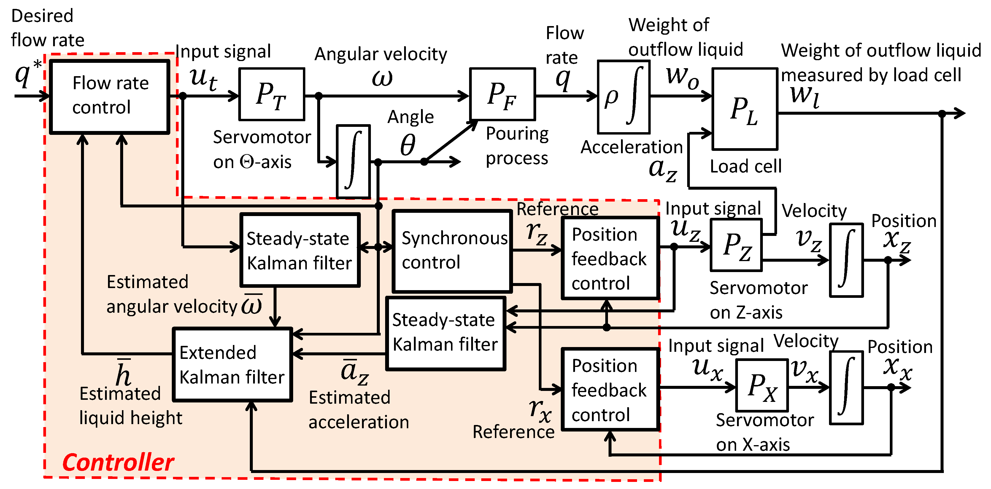
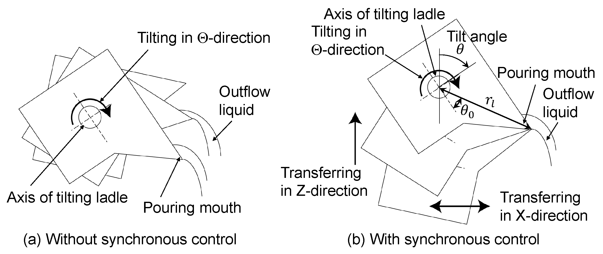
The entire control system for applying the flow rate control to the pouring machine is depicted in Figure 6. While implementing the flow rate control, it is required to acquire the liquid height at the pouring mouth of the ladle in real time; however, it is difficult to measure the liquid height of high-temperature molten metal using a liquid level meter. Therefore, a state estimation approach was applied to obtain the liquid height at the pouring mouth of the ladle. Furthermore, because the tilt axis of the ladle was located through the center of gravity of the ladle, the trajectory of the outflow liquid varied, as is depicted in Figure 7a. To solve this problem, the motions of the ladle along the X- and Z-axes are synchronously controlled with the motion along the $\Theta$-axis, as depicted in Figure 7b.

5.1. Synchronous Control

To suppress the variation in the trajectory of the outflow liquid, the center of the rotating ladle is shifted to the tip of the pouring mouth by achieving synchronous control in the X- and Z-directions [25]. The synchronous control is performed as

$$\begin{array}{c}\hfill r_x=r_{l}cos{\theta }_0-r_{l}cos({\theta }_0-\theta ),\end{array}$$

(23)

$$\begin{array}{c}\hfill r_z=r_{l}sin{\theta }_0-r_{l}sin({\theta }_0-\theta ),\end{array}$$

(24)

where $r_l$ denotes the length between the center of the rotational axis of the tilting ladle motor to the tip of the pouring mouth, as depicted in Figure 7b. Additionally, ${\theta }_0$ is the angle between $r_l$ and the horizontal line at the standing posture of the ladle. Furthermore, $r_x$ and $r_z$ are the reference positions on the X- and Z-axes, respectively. The position feedback control system is constructed using servomotors on those axes, and synchronous control can be accomplished by precisely tracking the ladle position, with respect to the reference values of $r_x$ and $r_z$.

5.2. State Estimation in an Automatic Pouring Machine

A Kalman filter was applied to estimate the state variables, such as the liquid height at the pouring mouth, the angular velocity of the tilting ladle, and the acceleration of transference on the Z-axis, as depicted in Figure 6. In this study, the state estimation approach is decomposed into two steady-state Kalman filters and one extended Kalman filter, for simple implementation of the state estimation approach in the automatic pouring machine.

The two steady-state Kalman filters are applied for estimating the state variables in the drive systems of the $\Theta$- and Z-axes, respectively. The plant model for estimating the state variables of the drive system on the $\Theta$-axis is denoted as follows:

$$\begin{array}{c}\hfill \left[\begin{array}{c}\dot{\theta }\\ \dot{\omega }\end{array}\right]=\left[\begin{array}{cc}0& 1\\ 0& -\frac{1}{T_t}\end{array}\right]\left[\begin{array}{c}\theta \\ \omega \end{array}\right]+\left[\begin{array}{c}0\\ \frac{K_t}{T_t}\end{array}\right]u_t,\end{array}$$

(25)

$$\begin{array}{c}\hfill y=\left[\begin{array}{cc}1& 0\end{array}\right]\left[\begin{array}{c}\theta \\ \omega \end{array}\right].\end{array}$$

(26)

The plant model on the Z-axis is formed in the same way as presented in Equations (25) and (26). Furthermore, in this study, the respective covariance matrices $Q_t$ and $R_t$ of the system noise and the measurement noise in the drive system of the $\Theta$-axis are given as follows:

$$\begin{array}{c}\hfill Q_t=\mathrm{diag}(1\times {10}^{-15},1\times {10}^{-1}),\end{array}$$

(27)

$$\begin{array}{c}\hfill R_t=1\times {10}^{-5}.\end{array}$$

(28)

The respective covariance matrices $Q_z$ and $R_z$ of the system noise and the measurement noise in the drive system of the Z-axis are also given as follows:

$$\begin{array}{c}\hfill Q_z=\mathrm{diag}(1\times {10}^{-3},1\times {10}^{-3}),\end{array}$$

(29)

$$\begin{array}{c}\hfill R_z=1\times {10}^{-7}.\end{array}$$

(30)

Further, the acceleration along the Z-axis can be estimated by estimating the state variables in the drive system of the Z-axis as

$${\overline{a}}_z=-\frac{1}{T_z}{\overline{v}}_z+\frac{K_z}{T_z}{u}_z,$$

(31)

where the variables with a bar represent the estimated variables.

In the design of the extended Kalman filter for estimating the state variables in the pouring process, the plant model can be denoted as follows:

$$\begin{array}{c}\hfill \left[\begin{array}{c}\dot{h}\\ {\dot{w}}_o\\ {\dot{w}}_l\end{array}\right]=\left[\begin{array}{c}-\frac{q\left(h\right)}{A\left(\theta \right)}-\frac{1}{A\left(\theta \right)}\left(\frac{\partial A\left(\theta \right)}{\partial \theta }+\frac{\partial V_s\left(\theta \right)}{\partial \theta }\right)\overline{\omega }\\ \rho q\left(h\right)\\ -\frac{1}{T_l}{w}_l+\frac{1}{T_l}\left(w_o-\frac{w_z}{g}{\overline{a}}_z\right)\end{array}\right],\end{array}$$

(32)

$$\begin{array}{c}\hfill y=\left[\begin{array}{ccc}0& 0& 1\end{array}\right]\left[\begin{array}{c}h\\ w_o\\ w_l\end{array}\right].\end{array}$$

(33)

In this study, the respective covariance matrices $Q_f$ and $R_f$ of the system noise and the measurement noise in the pouring process are given as follows:

$$\begin{array}{c}\hfill Q_f=\mathrm{diag}(2.5\times {10}^{-10},1\times {10}^{-11},1\times {10}^{-11}),\end{array}$$

(34)

$$\begin{array}{c}\hfill R_f=5\times {10}^{-4}.\end{array}$$

(35)

5.3. Model Parameter Identification

The model parameters of the drive systems of the X-, Z-, and $\Theta$-axes in the automatic pouring machine, as depicted in Figure 1b, were identified by fitting the simulations of the drive system models to the experimental data. The identified model parameters are presented in

Table 2. Identified model parameters for the drive systems of the X-, Z-, and $\Theta$-axes.

	X-Axis	Z-Axis	$\mathbf{\Theta }$-Axis
Gain, K	1.00	1.00	1.00
Time constant, T	0.050 s	0.050 s	0.022 s

.

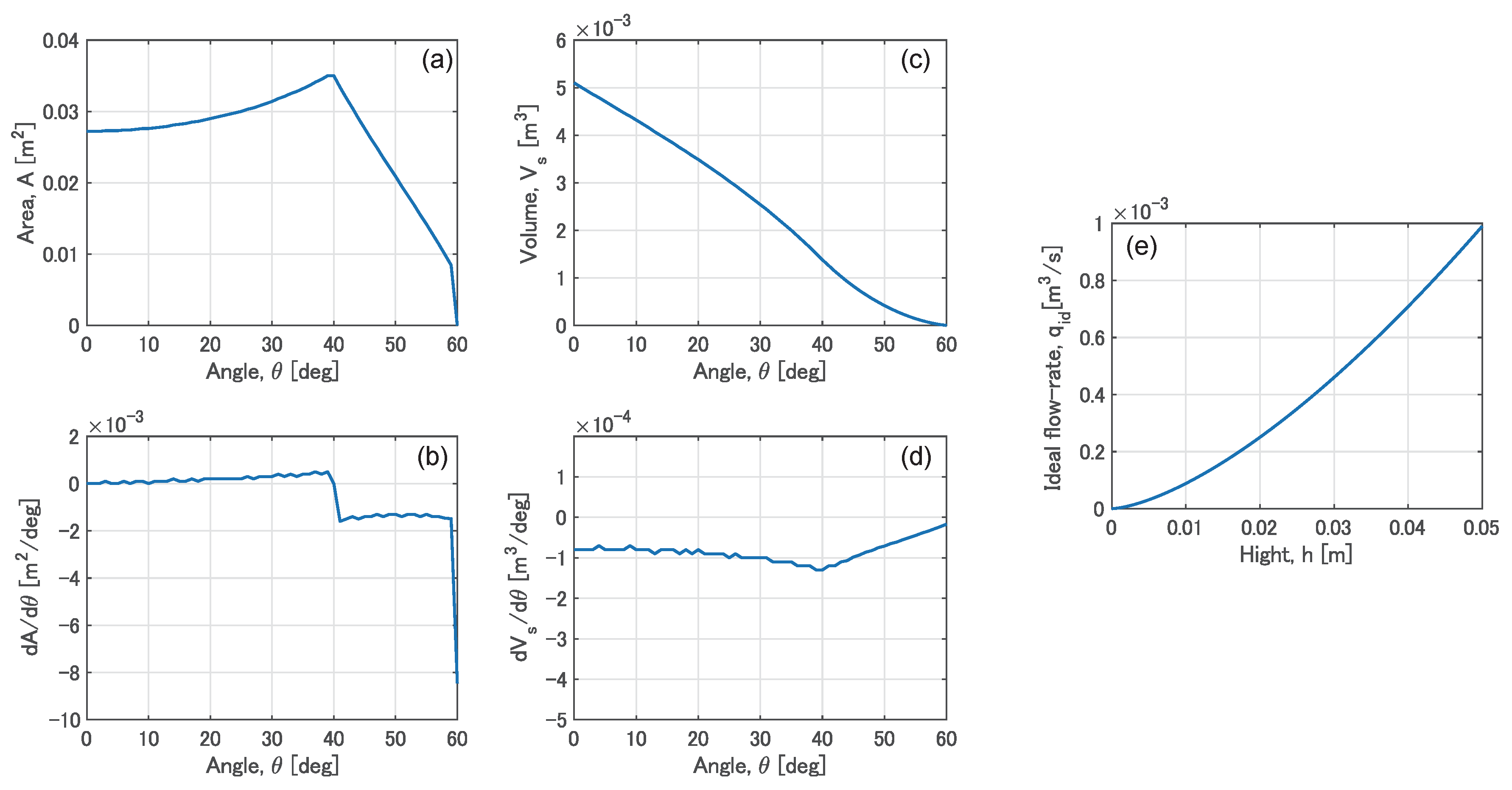
In the model parameters of the pouring process, the parameters $A\left(\theta \right)$, $V_s\left(\theta \right)$, and $q\left(h\right)$ are related to the shape of the ladle, as depicted in Figure 2, and can be obtained using CAD calculations. The obtained parameters are presented in Figure 8. Figure 8a,b denote the liquid plane area, which is horizontal to the pouring mouth, with respect to the tilt angle and its partial derivative with respect to the angle, respectively. Figure 8c,d show the liquid volume under the tip of the pouring mouth and its partial derivative, with respect to the tilt angle, and Figure 8e shows the ideal flow rate of the outflow liquid, with respect to the liquid height at the pouring mouth. The ideal flow rate is indicated as the flow rate coefficient $c=1$. Furthermore, the length between the center of the rotational axis of the tilting ladle motor and the tip of the pouring mouth, as depicted in Figure 7b, is obtained as $r_l=0.206$ m, by CAD calculation.

The flow rate coefficient, c, in the pouring process can be identified by fitting the simulation to the experimental data using the pouring model. In this study, the flow rate coefficient was obtained as $c=0.75$. The density of the liquid is given as $\rho ={10}^3$ kg/m³, as water is considered to be the target liquid in this study.

In the load cell model, the weight of the part transferred along the Z-axis is $w_z=18.6$ kg. Additionally, the time constant in the load cell was identified as $T_l=0.16$ s.

5.4. Control Parameters

In the design of the flow rate control, the damping ratio in Equation (18) is given as $\zeta =1$ for high tracking performance with suppressed vibration. In addition, we adjust the natural angular frequency ${\omega }_n$ in Equation (18). Further, the tracking performance can be improved by increasing the natural angular frequency. However, this can also increase the signal noise in the control loop. The natural angular frequency was determined as ${\omega }_n=2$ rad/s, in this study.

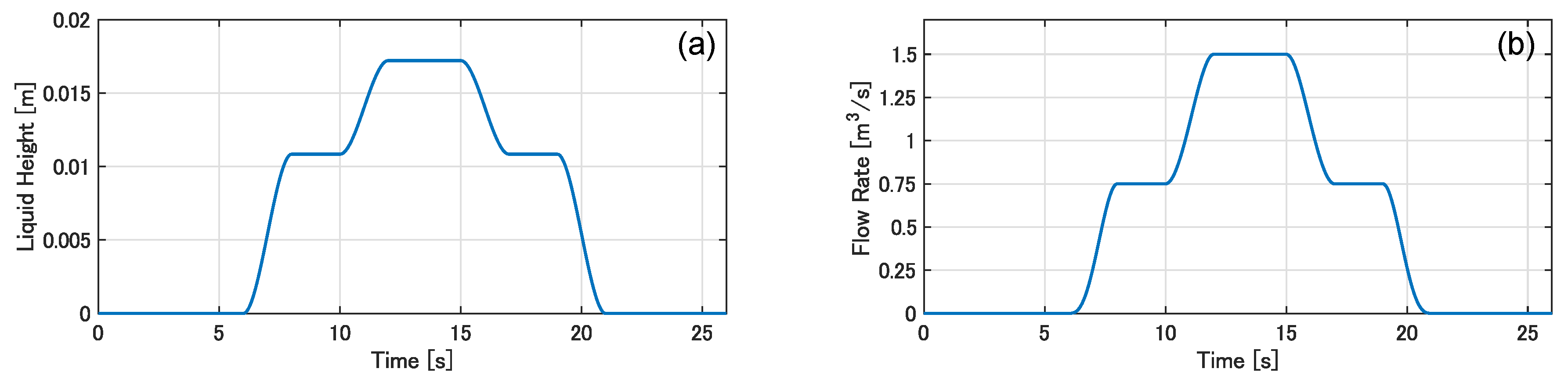
5.5. Design of the Reference Trajectory

In the experimental study, the target flow rate contains two stages, with $q_{f1}^{\ast }=0.75\times {10}^{-4}$ and $q_{f2}^{\ast }=1.50\times {10}^{-4}$ m³/s. The reference trajectory of the liquid height at the pouring mouth, by which the target flow rate can be achieved, is depicted in Figure 9.

Figure 9a denotes the reference trajectory of the liquid height, and Figure 9b shows the trajectory of the flow rate, which can be derived by substituting the reference trajectory of the liquid height, presented in Figure 9a, into Equation (6). As can be observed from Figure 9b, the flow rate from 8–10 s and from 17–19 s stays at $q_{f1}^{\ast }=0.75\times {10}^{-4}$ m³/s, and the flow rate from 12–15 s stays at $q_{f2}^{\ast }=1.50\times {10}^{-4}$ m³/s.

6. Experimental Verification

The developed flow rate control system was verified using experiments with the tilting-ladle-type automatic pouring machine depicted in Figure 1b. In the experiments, the developed flow rate control was compared with a conventional feed-forward flow rate control. The feed-forward flow rate control was constructed using the inverse of the pouring process model [3].

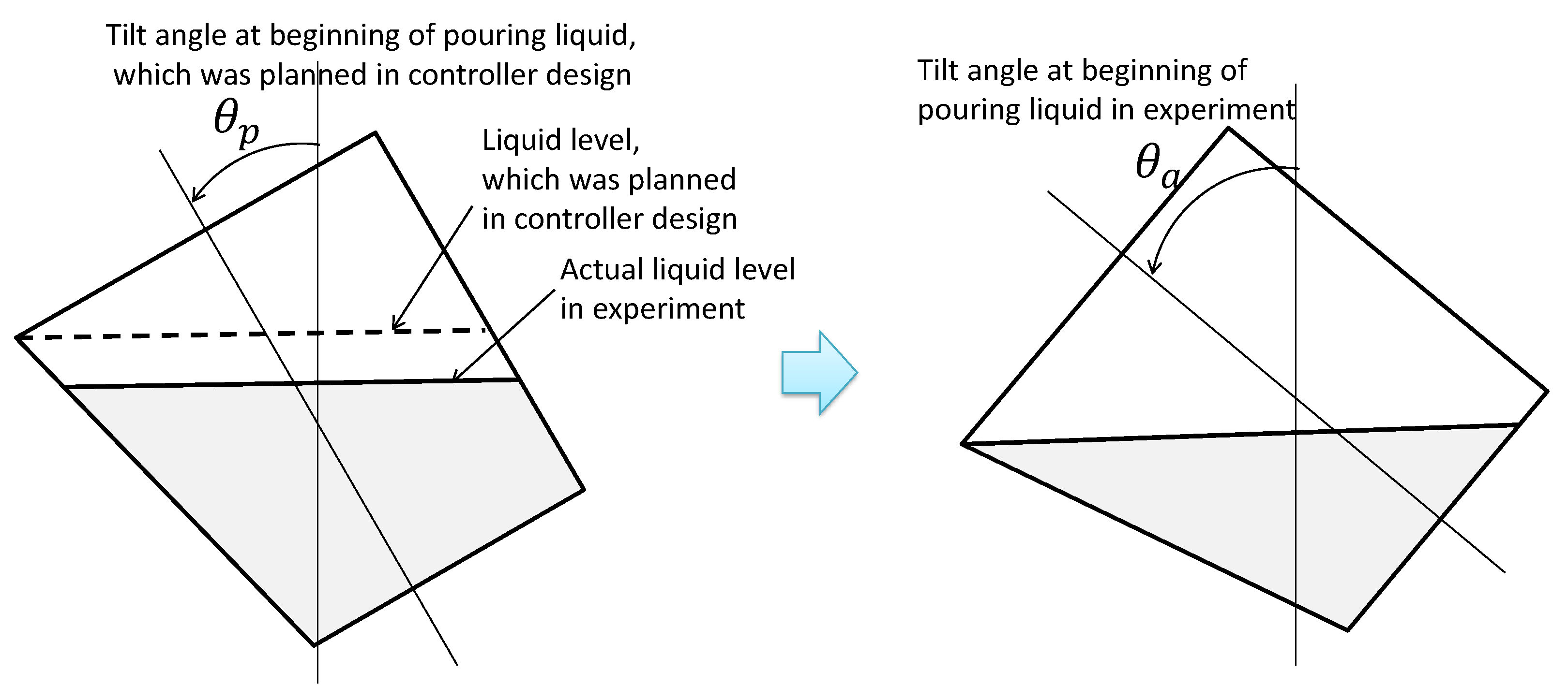
In the practical use of a tilting-ladle-type automatic pouring machine, it is difficult to precisely measure the ladle tilt angle at which the molten metal can be initially poured. This is because the starting condition for pouring the molten metal is influenced by the surface tension and density variations in the molten metal. Therefore, we assumed that majority of the disturbance in the flow rate control was caused by a difference between the tilt angles at the beginning of pouring the liquid in the experiments and the controller design.

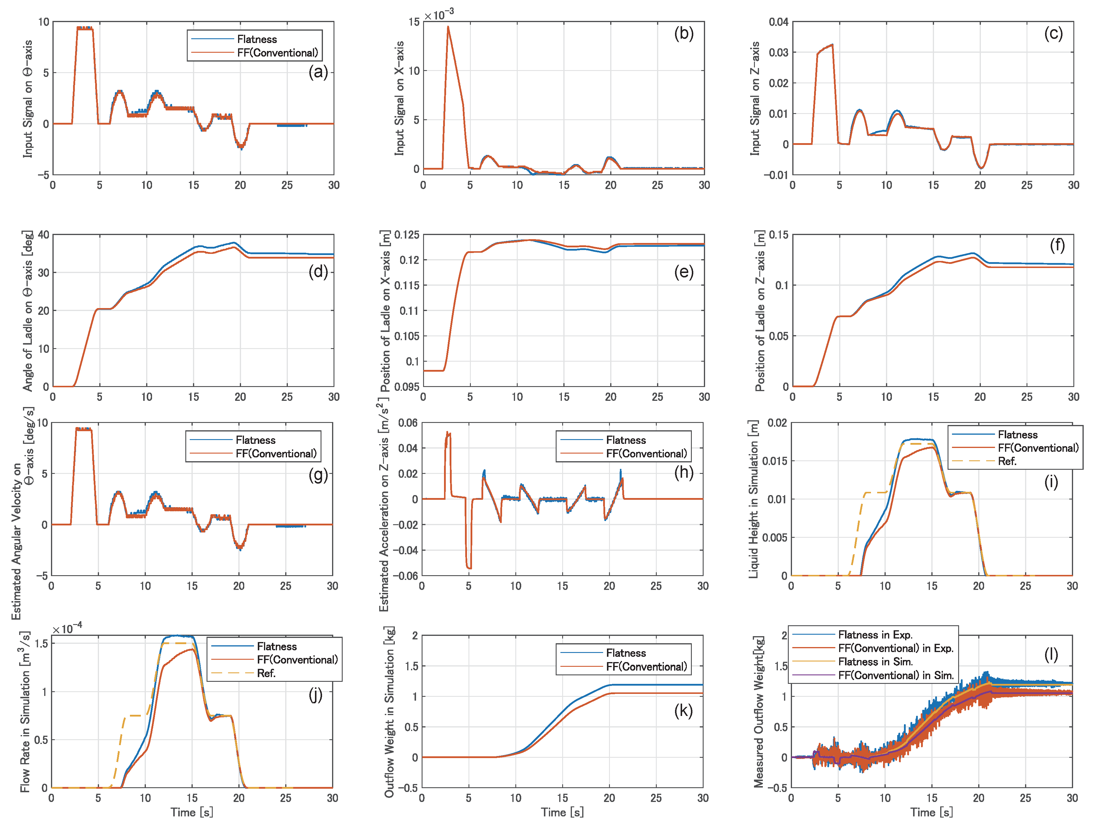
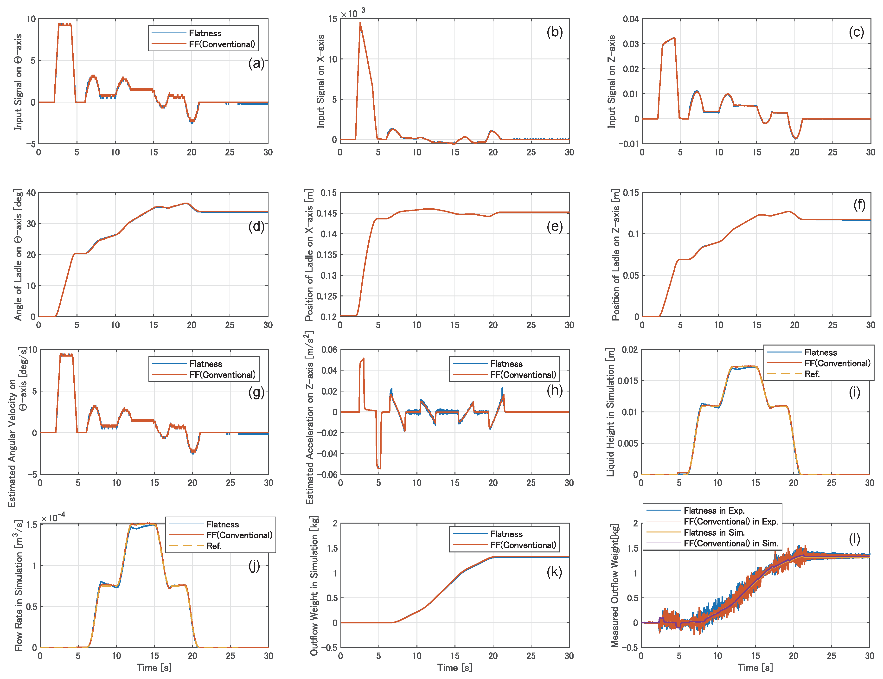
At first, we conducted experiments on the flow rate control without any disturbance; because there was no disturbance during the experiments, pouring the liquid from the ladle began according to the controller design, with $\theta =20$ deg. The experimental results are depicted in Figure 10.

Figure 10a–c show the input signals to the servomotors of the $\Theta$-, X-, and Z-axes, respectively. Figure 10d–f show the tilt angle of the ladle on the $\Theta$-axis and the positions of the ladle on the X- and Z-axes, respectively. Figure 10g,h show the angular velocity of the tilting ladle and the acceleration of the ladle along the Z-axis, respectively. These are estimated by the steady-state Kalman filters. Figure 10i–k denote the liquid height at the pouring mouth, the flow rate of the outflow liquid, and the weight of the outflow liquid, respectively, which were simulated by the pouring model with the input signals shown in Figure 10a–c. In Figure 10a–k, the blue and orange lines represent the results obtained using the developed flow rate control based on the differential flatness and the conventional feed-forward flow rate control, respectively. In Figure 10i–k, the broken yellow lines represent the reference trajectories, which are also presented in Figure 9. Figure 10l denotes the weight of the outflow liquid, which was measured using the load cell. In this graph, the blue and orange lines represent the experimental results obtained using the developed and conventional flow rate controls, respectively. The yellow and purple lines represent the simulation results obtained by the developed and conventional flow rate controls, respectively. As can be observed from Figure 10l, because the simulation results were fitted with the experimental results, the pouring process in the tilting-ladle-type automatic pouring machine can be precisely represented by using the pouring model derived in this study. Therefore, we observe the simulation results in Figure 10i–k as actual states in the automatic pouring machine. In the experiments on the pouring process without any disturbance, the liquid height at the pouring mouth and the flow rate of the outflow liquid in each flow rate control were precisely tracked to the reference trajectory.

We also conducted experiments on the pouring process with disturbance. The disturbance was applied, as depicted in Figure 11. The controller planned to begin pouring the liquid at a tilt angle of ${\theta }_p=20$ deg. However, pouring started at a tilt angle of ${\theta }_a=23.7$ deg in the experiments. The experimental results are depicted in Figure 12, which are presented in the same manner as in the Figure in Figure 10.

As can be observed from Figure 12i,j, the initial increases in the liquid height at the pouring mouth and the flow rate in each flow rate control were delayed by the disturbance. The tracking performances of the reference trajectories were improved by applying the flow rate control based on differential flatness to the automatic pouring machine.

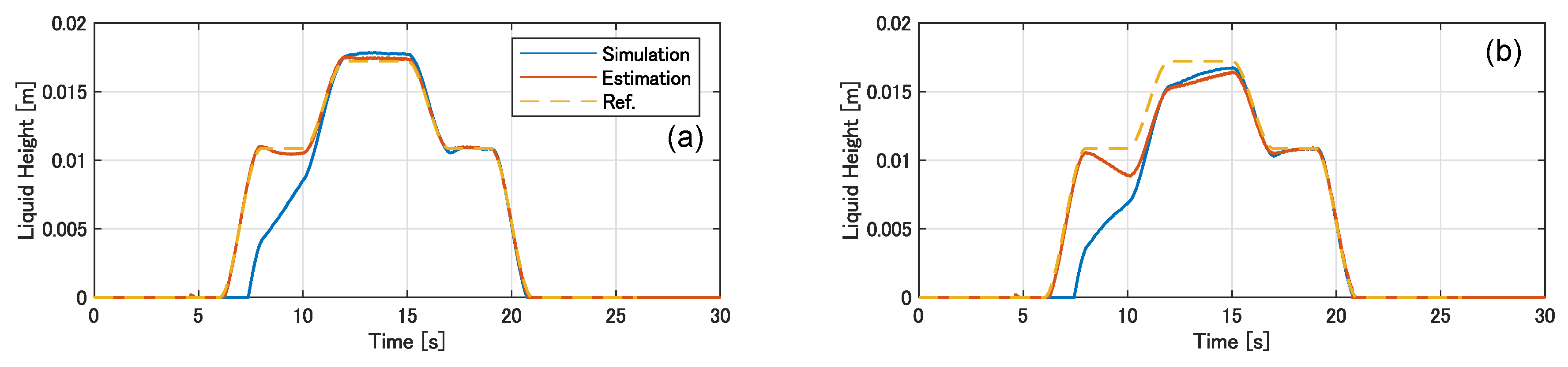
In Figure 13, we denote the results of the state estimation of the liquid height at the pouring mouth.

These results were obtained in the experiments using a pouring process with disturbance. Figure 12a,b denote the liquid heights at the pouring mouth, obtained by implementing the developed flow rate control based on the differential flatness and the conventional feed-forward flow rate control, respectively. In Figure 13, the blue lines represent the simulation results obtained from the pouring model, which are the same as the graph Figure 12i. The orange lines represent the estimation results obtained using the extended Kalman filter. The broken yellow lines represent the reference trajectories. As can be observed from Figure 13b, the extended Kalman filter caused the estimated trajectory to gradually converge with the actual trajectory. Furthermore, in Figure 13a, the estimated liquid height matches precisely with the reference trajectory. Therefore, majority of the tracking error was caused by the estimation error using the extended Kalman filter. The state estimation of the automatic pouring machine must be improved to more precisely track to a target flow rate in the developed control system.

7. Conclusions and Future Works

In this study, we addressed the manner in which flow rate control based on differential flatness can be applied to a tilting-ladle-type automatic pouring machine, and verified the efficacy of the developed flow rate control through various experiments. The following conclusions can be obtained:

• From the viewpoint of practical application, a SISO-nonlinear-type controller design based on differential flatness was applied, to ensure the flow rate control of the automatic pouring machine;
• while implementing the flow rate control using the feedback control scheme, it was necessary to measure the states of the automatic pouring machine—however, it is difficult to directly measure the states of high-temperature molten metal. Therefore, in this study, the Kalman filter approach was applied for estimating the state variables of the automatic pouring machine;
• the steady-state and extended Kalman filters were decomposed for simple construction of the state estimate of the automatic pouring machine;
• in the experiments related to the pouring process without disturbance, both the feed-forward flow rate control based on the inverse pouring model, and the flow rate control based on differential flatness, achieved a flow rate by which the outflow liquid precisely tracked with the reference trajectory: We conclude that the pouring model described in this study could precisely represent the actual pouring process in the automatic pouring machine;
• in the experiments on a pouring process with disturbance, the tracking performance of the flow rate in the pouring machine could be improved by implementing flow rate control based on differential flatness; and
• a majority of the tracking errors of the flow rate control based on differential flatness were caused by the estimation errors of the extended Kalman filter.

Furthermore, the following recommendations for future work can be obtained:

• To obtain high tracking performance, the state estimation approach of the pouring machine should be improved in future studies;
• in the developed flow rate control, the flow rate of the outflow liquid was indirectly controlled, based on the liquid height at the pouring mouth. If any disturbances were observed in the relation between the flow rate and the liquid height at the pouring mouth, the tracking performance of the flow rate control may have degraded. Further, direct flow rate control must be achieved to construct a high-precision automatic pouring machine; and
• in practical pouring processes, the characteristics of the pouring material are variable with temperature, the added substance, and so on. Therefore, a control approach with computational intelligence, such that the controller can be adapted autonomously to the pouring environment, should be developed in the future work.

References

1. Lindsay, W. Automatic pouring and metal distribution systems. Foundry Trade J. 1983, 10, 151–176. [Google Scholar]
2. Terashima, K.; Miyoshi, T.; Noda, Y. Innovative automation technologies and IT applications of the metal casting process necessary for the foundries of the 21st century. Int. J. Autom. Technol. 2008, 2, 229–240. [Google Scholar] [CrossRef]
3. Noda, Y.; Nishida, T. Precision analysis of automatic pouring machines for the casting industry. Int. J. Autom. Technol. 2008, 2, 241–246. [Google Scholar] [CrossRef]
4. Neumann, E.; Trauzeddel, D. Pouring systems for ferrous applications. Foundry Trade J. 2002, 23–24. [Google Scholar]
5. Tayode, A.; Chitre, A.; Rahulkar, A. PLC based hydraulic auto ladle system. Int. J. Eng. Res. Appl. 2014, 4, 19–22. [Google Scholar]
6. Rajput, N.; Patil, N.; Sutar, M. Precision analysis and control of automatic pouring machine to control the flow ability to minimize the porosity of SG200 casting for foundry. Int. J. Res. Adv. Technol. 2015, 3, 22–24. [Google Scholar]
7. Voss, T. Optimization and control of modern ladle pouring process. In Proceedings of the 73rd World Foundry Congress, Cracow, Poland, 23–27 September 2018; pp. 497–498. [Google Scholar]
8. Noda, Y.; Terashima, K. Modeling and feedforward flow rate control of automatic pouring system with real ladle. Int. J. Robot. Mechatron. 2007, 19, 205–211. [Google Scholar] [CrossRef]
9. Noda, Y.; Watari, H.; Yamazaki, T. Control of liquid level in tundish of strip caster with automatic pouring system. Mater. Sci. Forum 2008, 575–578, 147–153. [Google Scholar] [CrossRef]
10. Yano, K.; Terashima, K. Supervisory control of automatic pouring machine. Control Eng. Pract. 2010, 18, 230–241. [Google Scholar] [CrossRef]
11. Tsuji, T.; Noda, Y. High-precision pouring control using online model parameters identification in automatic pouring robot with cylindrical ladle. In Proceedings of the 2014 IEEE International Conference on Systems, Man, and Cybernetics, San Diego, CA, USA, 5–8 October 2014; pp. 2593–2598. [Google Scholar]
12. Kuriyama, Y.; Yano, K.; Nishido, S. Optimization of pouring velocity for aluminium gravity casting. In Fluid Dynamics, Computational Modeling and Applications; Juarez, L., Ed.; InTech: Rijeka, Croatia, 2012; pp. 575–588. [Google Scholar]
13. Pan, Z.; Park, C.; Manocha, D. Robot motion planning for pouring liquids. In Proceedings of the 26th International Conference on Automated Planning and Scheduling, London, UK, 12–17 June 2016; pp. 518–526. [Google Scholar]
14. Li, L.; Wang, C.; Wu, H. Research on kinematics and pouring law of a mobile heavy load pouring robot. Math. Prob. Eng. 2018, 2018, 8790575. [Google Scholar] [CrossRef]
15. Sueki, Y.; Noda, Y. Operational assistance system with direct manipulation of flow rate and falling position of outflow liquid in tilting-ladle-type pouring machine. In Proceedings of the 73rd World Foundry Congress, Cracow, Poland, 23–27 September 2018; pp. 325–326. [Google Scholar]
16. Schenck, C.; Fox, D. Visual closed-loop control for pouring liquids. In Proceedings of the IEEE International Conference on Robotics and Automation, Singapore, 29 May–3 June 2017; pp. 2629–2636. [Google Scholar]
17. Do, C.; Burgard, W. Accurate pouring with an autonomous robot using an RGB-D camera. In Intelligent Autonomous Systems 15, Proceedings of the International Conference on Intelligent Autonomous Systems, Baden-Baden, Germany, 11–15 June 2018; Springer: Cham, Switzerland, 2018; pp. 210–221. [Google Scholar]
18. Kennedy, M.; Schmeckpeper, K.; Thakur, D.; Jiang, C.; Kumar, V.; Daniilidis, K. Autonomous Precision Pouring From Unknown Containers. IEEE Robot. Autom. Lett. 2019, 4, 2317–2324. [Google Scholar] [CrossRef]
19. Kennedy, M.; Queen, K.; Thakur, D.; Daniilidis, K.; Kumar, V. Precise dispensing of liquids using visual feedback. In Proceedings of the 2017 IEEE/RSJ International Conference on Intelligent Robots and Systems, Vancouver, BC, Canada, 24–28 September 2017. [Google Scholar] [CrossRef]
20. Noda, Y.; Terashima, K. Estimation of flow rate in automatic pouring system with real ladle used in industry. In Proceedings of the ICROS-SICE Internaonal Conference, Fukuoka, Japan, 18–21 August 2009; pp. 354–359. [Google Scholar]
21. Noda, Y.; Birkhold, M.; Terashima, K.; Sawodny, O.; Verl, A. Flow rate estimation using Unscented Kalman Filter in automatic pouring robot. In Proceedings of the SICE Annual Conference, Tokyo, Japan, 13–18 September 2011; pp. 769–774. [Google Scholar]
22. Noda, Y.; Zeitz, M.; Sawodny, O.; Terashima, K. Flow rate control based on differential flatness in automatic pouring robot. In Proceedings of the IEEE International Conference on Control Applications, Denver, CO, USA, 3–5 March 2011; pp. 1468–1475. [Google Scholar]
23. Ito, A.; Oetinger, P.; Tasaki, R.; Sawodny, O.; Terashima, K. Visual nonlinear feedback control of liquid level in mold sprue cup by cascade system with flow rate control for tilting-ladle-type automatic pouring system. Mater. Sci. Forum 2018, 925, 483–490. [Google Scholar] [CrossRef]
24. Ramirez, H.; Agrawal, S. SISO nonlinear systems. In Differentially Flat Systems; Lewis, F., Ed.; CRC Press: Boca Raton, FL, USA, 2004; pp. 191–220. [Google Scholar]
25. Terashima, K.; Yano, K.; Sugimoto, Y.; Watanabe, M. Position control of ladle tip and sloshing suppression during tilting motion in automatic pouring machine. In Proceedings of the 10th IFAC symposium on Automation in Mining, Mineral and Metal Processing, Tokyo, Japan, 4–6 September 2001; pp. 182–187. [Google Scholar]
Figure 1. Photos of tilting-ladle-type automatic pouring machines. (a) An automatic pouring machine that is actually applied in a casting plant, and (b) the automatic pouring machine that has been developed in the present laboratory of the authors.
Applsci 09 01978 g001
Figure 2. Shape of ladle used in this study.
Applsci 09 01978 g002
Figure 3. Signal diagram for the tilting-ladle-type automatic pouring machine. (a) Drive system of the Θ -axis, with pouring process and load cell; (b) drive system of the Z-axis; and (c) drive system of the X-axis.
Applsci 09 01978 g003
Figure 4. Geometric parameters of pouring process. (a) Parameters related to the ladle shape, and (b) parameters related to the pouring mouth.
Applsci 09 01978 g004
Figure 5. Signal diagram of flow rate control based on differential flatness.
Applsci 09 01978 g005
Figure 6. Signal diagram of the entire control system for applying flow rate control to the tilting-ladle-type automatic pouring machine.
Applsci 09 01978 g006
Figure 7. Illustrations of ladle motions in the X- and Z-directions, controlled synchronously to tilt the ladle in the Θ -direction: (a) Ladle motion without synchronous control, and (b) ladle motion with synchronous control.
Applsci 09 01978 g007
Figure 8. Model parameters related to the ladle shape. (a) Area of liquid plane which is horizontally located on the pouring mouth, A ( θ ) . (b) Partial derivative of the area A ( θ ) , with respect to the angle θ . (c) Liquid volume under the tip of the pouring mouth, V s ( θ ) . (d) Partial derivative of area V s ( θ ) , with respect to the angle θ . (e) Ideal flow rate q i d of the outflow liquid, with respect to the liquid height h at the pouring mouth.
Applsci 09 01978 g008
Figure 9. Reference trajectories in flow rate control. (a) Reference trajectory of liquid height at pouring mouth, which is added to the flow rate control. (b) Trajectory of flow rate, which is derived by substituting the reference trajectory of liquid height, presented in (a), into Equation (6).
Applsci 09 01978 g009
Figure 10. Experimental results of flow rate control to pouring process without disturbance. (a) Input signal added to motor of the Θ -axis. (b) Input signal added to motor of the X-axis. (c) Input signal added to motor of the Z-axis. (d) Angle of tilting ladle on Θ -axis. (e) Position of ladle on X-axis. (f) Position of ladle on Z-axis. (g) Angular velocity on Θ -axis, estimated by steady-state Kalman filter. (h) Acceleration on Z-axis, estimated by steady-state Kalman filter. (i) Liquid height at pouring mouth in simulation, using pouring model. (j) Flow rate of outflow liquid in simulation, using pouring model. (k) Weight of outflow liquid in simulation, using pouring model. (l) Weight of outflow liquid, measured by load cell.
Applsci 09 01978 g010
Figure 11. Illustration of the disturbance applied in the experiments, which was caused by a difference between the tilt angles at the beginning of pouring the liquid in the experiments and the controller design.
Applsci 09 01978 g011
Figure 12. Experimental results of flow rate control to pouring process with disturbance. (a) Input signal added to motor of the Θ -axis. (b) Input signal added to motor of the X-axis. (c) Input signal added to motor of the Z-axis. (d) Angle of tilting ladle on Θ -axis. (e) Position of ladle on X-axis. (f) Position of ladle on Z-axis. (g) Angular velocity on Θ -axis, estimated by steady-state Kalman filter. (h) Acceleration on Z-axis, estimated by steady-state Kalman filter. (i) Liquid height at pouring mouth in simulation, using pouring model. (j) Flow rate of outflow liquid in simulation, using pouring model. (k) Weight of outflow liquid in simulation, using pouring model. (l) Weight of outflow liquid, measured by load cell.
Applsci 09 01978 g012
Figure 13. Comparative results of liquid height at pouring mouth. (a) Liquid height in developed flow rate control. (b) Liquid height in conventional feed-forward flow rate control.
Applsci 09 01978 g013