Layer-Level Knowledge Distillation for Deep Neural Network Learning

Abstract

Motivated by the recently developed distillation approaches that aim to obtain small and fast-to-execute models, in this paper a novel Layer Selectivity Learning (LSL) framework is proposed for learning deep models. We firstly use an asymmetric dual-model learning framework, called Auxiliary Structure Learning (ASL), to train a small model with the help of a larger and well-trained model. Then, the intermediate layer selection scheme, called the Layer Selectivity Procedure (LSP), is exploited to determine the corresponding intermediate layers of source and target models. The LSP is achieved by two novel matrices, the layered inter-class Gram matrix and the inter-layered Gram matrix, to evaluate the diversity and discrimination of feature maps. The experimental results, demonstrated using three publicly available datasets, present the superior performance of model training using the LSL deep model learning framework.

1. Introduction

Convolutional neural networks (CNN) of deep learning have proved to be very successful in many applications in the field of computer vision, such as image classification [1], object detection [2,3,4], semantic segmentation [5], and others. However, the large network structure also brings high computational complexity and memory cost. This problem motivates researchers to develop model compression methods for neural networks. Model compression methods can be roughly divided into two categories: network pruning [6,7,8,9,10] and knowledge distillation (KD) methods [11,12,13,14,15]. Network pruning methods reduce the number of weights or neurons during neural network training, whereas knowledge distillation methods train a small model linked to a large model, which is also called a teacher–student network. The core idea of knowledge distillation is to consider not only the supervision of information from the large model that can be transferred to the neurons of the small model, but also the output of the small network, which should be as similar as possible to the output of the large network.

Applications of network pruning and knowledge distillation include reducing power consumption on mobile devices [16,17,18], object detection [19], visual relationship detection [20,21], and character recognition [22]. One-shot whole network compression [16] compresses the CNN network to deploy deep CNNs on mobile devices. However, model compression methods learn compact models, but with reduced accuracy. In [19], a new framework was proposed to learn compact and fast object detection networks with improved accuracy using knowledge distillation and hint learning.

In this paper, we propose a new Layer Selectivity Learning (LSL) framework to tackle the knowledge distillation method to transfer information from a well-trained large CNN model to a smaller CNN model in a layer-level manner. This leads to a compact and small model with higher accuracy than one that is trained alone. We exploit a teacher–network framework called Auxiliary Structure Learning (ASL) to link a well-trained large model, such as AlexNet [23], with a small new model within one unified learning framework. This can be achieved by projection layers and alignment layers. Then, two novel operators are proposed to select the corresponding intermediate layers automatically to link both models: the layered inter-class Gram matrix and the inter-layered Gram matrix. The former matrix uses feature maps within the same layer to obtain the relationships between classes. Each entry in the layered inter-class Gram matrix indicates the relationship of two classes to be highly correlated or irrelevant. The latter matrix calculates the Gram matrix using all feature vectors of two adjacent layers. The matrix represents whether the network can learn more diverse features than those in the previous layer. The contribution of the LSL framework is two-fold:

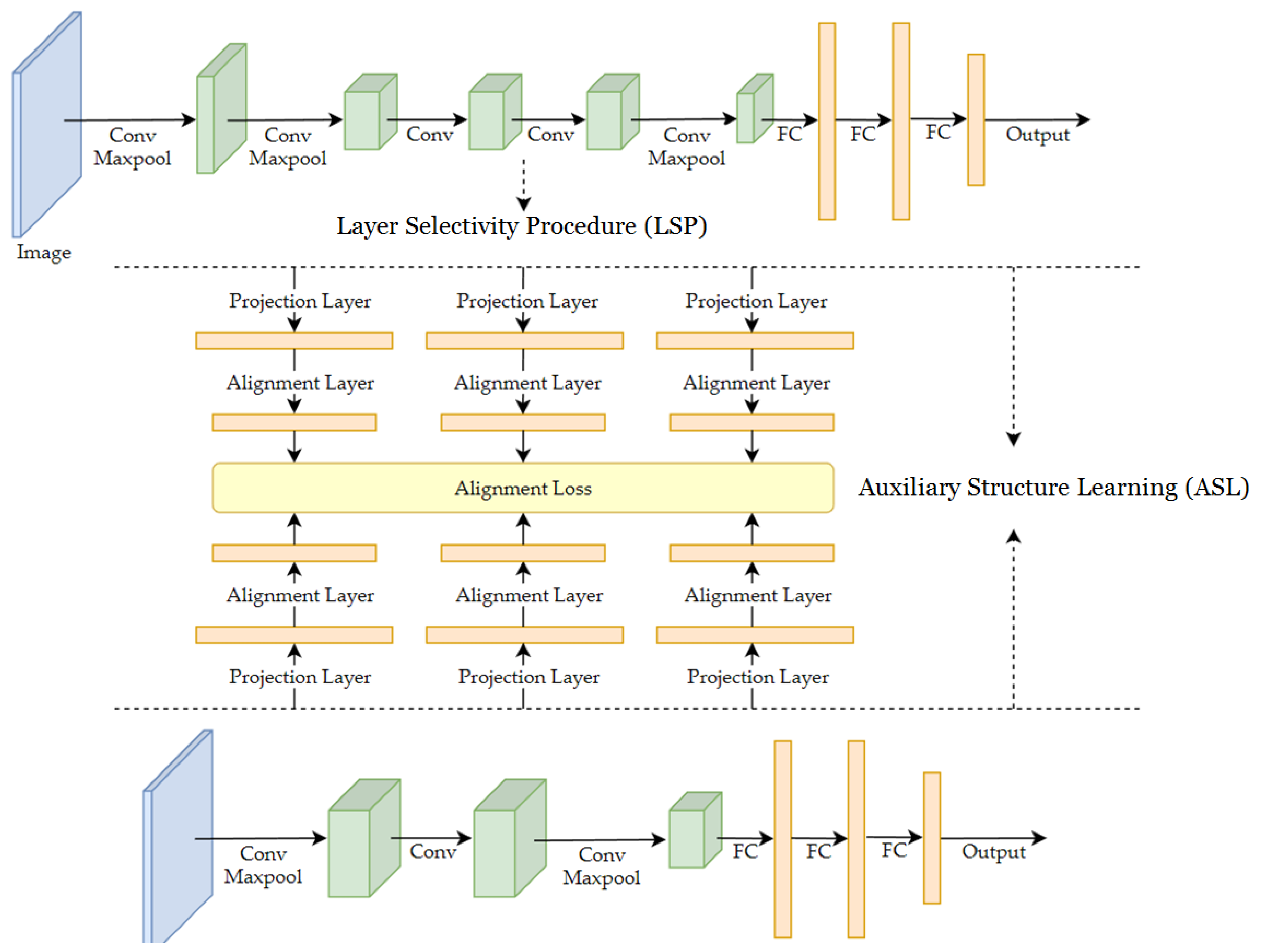
• Auxiliary Structure Learning (ASL) is proposed to improve the performance of a target model by distilling knowledge from a well-trained model;
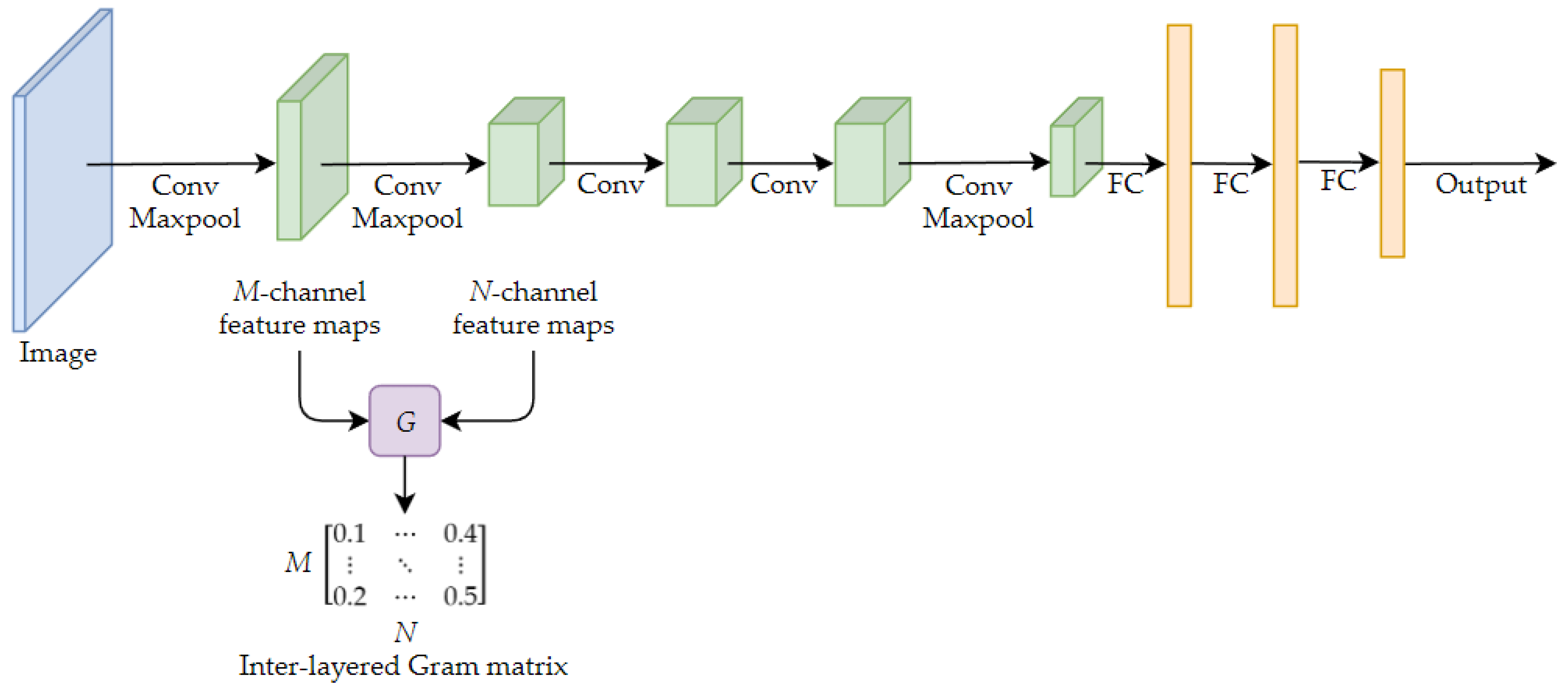
• The Layer Selectivity Procedure (LSP) includes two novel operators, the layered inter-class Gram matrix and the inter-layered Gram matrix, which are proposed for the selection and linkage of the intermediate layers of both target and source models.

The experimental results are demonstrated on three publicly available datasets, and show significant improvement in classification accuracy compared to other recently developed transfer learning methods. The rest of paper is organized as follows. The literature review of model compression and knowledge distillation is introduced in Section 2. In Section 3, the proposed Auxiliary Structure Learning (ASL) and the Layer Selectivity Procedure (LSP) are presented. The experimental settings and the results are demonstrated in Section 4. Lastly, Section 5 concludes our paper.

2. Related Work

2.1. Model Compression by Network Pruning

Large neural networks have a large number of weights. This means that large models are usually computationally expensive and require high memory and storage costs. So, it is important to reduce the model sizes. As wearable devices have become more and more popular in recent years, deep learning models are likely to be deployed in environments with limited memory and computation power in many applications. Model compression is critical for deep models applied in mobile devices and embedded systems.

Han et al. [24] proposed a model compression method to reduce the number of weights based on the idea of learning only the important connections in neural networks. In addition, Han et al. [13] propose pruning, quantization, and Huffman encoding methods to reduce the computational consumption of large networks. They first pruned the network by learning only the important connections. Then, weights were clustered to generate the code book. This approach aimed to enforce a weight sharing scheme. Lastly, Huffman encoding was applied to the weights and indices for further compression.

2.2. Knowledge Distillation

Deep convolutional neural networks are successful in many computer vision tasks. However, deep models contain a large number of weights and introduce high computational complexity for training. Therefore, researchers are dedicated to developing smaller network architectures while maintaining good performance. Knowledge distillation introduces the concept of distilling the knowledge of a well-trained large model and being able to transfer the knowledge to a relatively small model. In other words, it mimics a complex network by learning a simpler network with a similar performance. In the literature, the large model is usually called the source model or teacher model, whereas the small model is referred to as the target model or student model. The knowledge distillation methods can be divided into three categories: (1) knowledge distillation from output, (2) knowledge distillation from a single layer, and (3) knowledge distillation from multiple layers. We introduce these methods in the following sub-sections.

2.2.1. Knowledge Distillation from Output

Hinton et al. [7] proposed a knowledge distillation method by learning the soft target. The soft target is the class probabilities provided by the output of the final softmax function from the source model. On the contrary, the hard target is the output of the classifier. It is the final class label with the highest probability.

The soft target provides more information for model training. It can be used to restore intra-class variance and inter-class distance. To obtain the soft target, a new softmax function is defined with an additional parameter T. The parameter T is used to control the size difference between the different classes. They use the source model to generate probabilities of classes as soft target so that the small model can learn not only hard target but also the soft target to obtain the distribution of the input data. Finally, the small model is trained to minimize the cross-entropy loss of the hard target and the soft target. The weights are adjusted by the two targets to achieve knowledge distillation.

Model distillation methods help transfer the knowledge of large networks to small networks. However, it can be applied to a classification task only. Later, Huang et al. [8] proposed a knowledge distillation method called Neuron Selectivity Transfer (NST). This method accelerates the learning of neural networks and compresses the number of parameters. In addition, it helps in learning features of other computer vision tasks, such as object detection. However, it is still crucial to determine which layer is to be used as the intermediate presentation.

2.2.2. Knowledge Distillation from a Single Layer

Although the above knowledge distillation method can transfer knowledge from source models to target models, it only considers the output of the source model. In the case that the target model is very deep, it meets the difficulty of convergence problems. Romero et al. [9] proposed an improved method by introducing intermediate-level hints. In addition to the knowledge distillation of the final output of the model, their method also considers the output of one middle layer of the model. The core idea of the method is to enable the target model to learn the intermediate representation from the source model. The middle layer of the source model is called the hint layer and that of the target model is called the guided layer. To link both intermediate layers of the source and target models, it must be taken into account that the dimensions of the intermediate output of both models are usually different. A mapping function is introduced to ensure that the two dimensions can be projected to be the same dimension. Lastly, knowledge distillation is carried out by minimizing the loss function of the middle layer and output layer. However, these methods are limited and can be only applied to classification tasks.

2.2.3. Knowledge Distillation from Multiple Layers

Yim et al. [10] proposed another concept of knowledge distillation which employs the relationship between layers. The relationship between layers is considered to be more representative of the knowledge than the model output. Therefore, the extracted feature maps from two layers are used to generate the Flow of Solution Procedure (FSP) matrix. This represents the relationship between layers. By minimizing the distance between both FSP matrices of the source network and target network, this approach enforces the knowledge of source model to be transferred to the target model.

2.3. Alignment Layers

The concept of the alignment layer is firstly introduced in the cross-domain adaptation problem. Chen et al. [25] proposed a double-path deep domain adaptation network (DDAN) with fine-grained clothing attributes. The top path is defined by images from clothing shops as a source domain. The bottom path is employed for clothing images from streets as the target domain. An alignment layer is proposed between the two paths to enforce similarity between the parameters of both models. This means that this method can effectively make the features of two different domains similar. This motivated us to apply alignment layers to the transfer learning problem as the bridge between two deep learning models. Our method is different from previous works. By using the Layer Selectivity Procedure (LSP), knowledge can be transferred from one or more layers based on the analysis of the diversity and discrimination of feature maps in a layer-wise manner.

3. Proposed Method

We propose a novel Layer Selectivity Learning (LSL) framework, as shown in Figure 1. The LSL framework consists of two parts: (1) Auxiliary Structure Learning (ASL)—a new deep model learning scheme to train the target model with the help of a source model; (2) Layer Selectivity Procedure (LSP)—a scheme that can determine the corresponding intermediate layers of the source and target models automatically by two matrices, the layered inter-class Gram matrix and the inter-layered Gram matrix. We introduce both parts in the next sub-sections in detail.

3.1. Auxiliary Structure Learning (ASL)

Inspired by Chen et al. [25], we propose the Auxiliary Structure Learning framework [14]. It is an asymmetric dual-path learning framework, consisting of four components: (1) teacher network, (2) student network, (3) alignment layers, and (4) projection layers.

• Teacher network. The teacher network is also known as the source network, and is a well-trained deep learning model. In the ASL framework, the teacher network is supplied with pre-trained weights before the student network starts to train.
• Student network. The student network is also known as the target network. A student network is a new deep learning model without pre-trained weights.
• Alignment layer. The alignment layer is used to bridge the dual path deep learning models. It is designed to be the loss function that enforces similarity between two corresponding intermediate layers of both models.
• Projection layer. Since any two intermediate layers of both the teacher and student models are not likely to have the same feature dimensions, they cannot align directly. Before the representation layer connects to the alignment layer, it needs to connect to one additional fully connected layer, which is called the projection layer. This ensures that the two intermediate layers are projected to same dimension.

In the ASL framework, the teacher network can be considered as auxiliary architecture to train the student network. The choice of the teacher network is flexible, since we can choose any well-known deep model according to the requirement of our task, such as AlexNet [11] or VGGNet [16]. For the student network, it can be any new model without pre-trained weights. To link the layer of the teacher model to the layer of the student model, projection layers are required to project both layers to the same dimension. In fact, the fully connected layer is exploited as the projection layer in the ASL framework. After connecting to the projection layers, the alignment layer is introduced to build dependencies of both models. Alignment loss is in following form:

$${ℒ}_{\mathit{Align}}^{\left(k\right)}\left(t,s\right)=\Vert X_t^{\left(i\right)} {-X}_s^{\left(j\right)}{\Vert }_2$$

(1)

where $t$ and $s$ represent the teacher network and the student network, respectively. $X_t^{\left(i\right)}$ and $X_s^{\left(j\right)}$ are the feature representations from the i-th and j-th layers of the teacher network and the student network, respectively. $k$ is the index of the alignment layer. By minimizing ${ℒ}_{\mathit{Align}}^{\left(k\right)}\left(t,s\right)$, it enforces the j-th intermediate layer of the student model to be similar to the i-th intermediate layer of the teacher model. This transfers knowledge from the teacher network to the student network. The benefits to the student network are accuracy improvement and fast convergence, compared to the network when it is trained alone.

The total loss function of the ASL framework can be defined as follows:

$${ℒ}_{\mathit{total}}={{\displaystyle \sum }}_{k=1}^n{ℒ}_{\mathit{Align}}^{\left(k\right)}\left(t,s\right)+{{\displaystyle \sum }}_{p=1}^m{ℒ}_{\mathit{model}}^{\left(p\right)}(y,z)$$

(2)

where ${ℒ}_{\mathit{Align}}^{\left(k\right)}\left(t,s\right)$ is alignment loss, n is the total number of alignment layers. If n = 3, it means that the teacher model and the student model are linked by three intermediate layers. ${ℒ}_{\mathit{model}}^{\left(p\right)}\left(y,z\right)$ is the model loss term. p is the index of the deep models. m represents the total number of models in the ASL framework. In our dual-path deep model framework, there are two models, the teacher model and the student model. Therefore, m = 2. The model loss term is defined as follows:

$${ℒ}_{\mathit{model}}^{\left(p\right)}\left(y,z\right)=\log \left({\displaystyle \sum }_{j=1}^{}{e}^{z_j}\right)-y$$

(3)

where $z_j$ is the j-th prediction result and y is the label for input data. ${ℒ}_{\mathit{total}}$ represents the total loss by considering the loss of the teacher and student models and the loss of all alignment layers. This indicates that the teacher and student models are trained simultaneously in the training stage.

3.2. Layer Selectivity Procedure (LSP)

One issue remains in the ASL framework. The intermediate layer of the teacher model is linked to the layer of the student model via the projection layer and alignment layer. How can we select the intermediate layer from the teacher network and one corresponding intermediate layer from the student network to link both models? In this section, a novel scheme, the Layer Selectivity Procedure (LSP), is proposed to determine the intermediate layers and bind the two models. Two matrices, the layered inter-class Gram matrix and the inter-layered Gram matrix, are proposed to help select the appropriate layers from the teacher and student models. Then, the projection layers and alignment layers can be later deployed to build the ASL framework.

3.2.1. Inter-Layered Gram Matrix

Inspired by Gatys et al. [10], the Gramian matrix is capable of representing the texture information of the input image, because it is generated by calculating the inner product of feature vectors. The directionality between features can be considered as the similarity of texture information. The Gramian matrix that computes the inner product of features from adjacent layers is referred to as the inter-layered Gram matrix. The value in the entry of the inter-layered Gram matrix (i, j) is equal to the inner product of the i-th channel and the j-th channel in the deep learning model. The large value of the inner product means two feature vectors are more aligned to the same direction. Features extracted from that layer are considered to carry less information. We use the inter-layered Gram matrix to represent the relationship between feature maps between two layers and consider the layer diversity. The layer with more diversity, between the inter-layered Gram matrix and its previous layer, is more likely to be chosen as the alignment layer. The illustration of the procedure employed to determine the inter-layered Gram matrix is depicted in Figure 2.

For a given trained CNN model, feature maps can be extracted from the convolutional and fully-connected layers. Then, we compute the inner product of feature vectors from two layers to obtain the inter-layered Gram matrix $G_{m,n}^l\in {ℝ}^{M\times N}$. For a given layer $l$ and its previous layer $l-1$, the feature maps can be denoted as $F^{l-1}\in {ℝ}^{K\times M}$ and $F^l\in {ℝ}^{K\times N}$, where $M$ and N are the number of channels in layer $l-1$ and layer $l$. m and n are the index of the channels in layer $l-1$ and layer $l$, respectively. $K$ is the 1D feature dimension of the feature map. In practice, reshaping the feature maps into one dimension with zero padding is required to ensure that the feature vectors are in the same dimension. The (m, n) entry of the inter-layered Gram matrix $G_{m,n}^l$ can be defined as follows:

$$G_{m,n}^l=\frac{F_m^{l-1}{,F}_n^l}{K}.$$

(4)

The feature diversity can be calculated for a given layer $l$ by:

$$G_{\mathit{diversity}}^l=\frac{{{\displaystyle \sum }}_m{{\displaystyle \sum }}_n{G}_{m,n}^l}{M\times N}.$$

(5)

The entry of the inter-layered Gram matrix represents the relationship between two layers. A value close to zero indicates that features learned through the adjacent layers are not aligned and thus more diverse. A smaller value of $G_{\mathit{diversity}}^l$ indicates that layer $l$ contains more distinctive features. Note that the values of feature maps obtained by the activation function ReLu are non-negative. Therefore, the values of the inter-layered Gram matrix range from 0 to 1. Then, the layer with minimal values of $G_{\mathit{diversity}}^l$ is chosen as the representative intermediate layer. The optimization can be represented as follows:

$$l^{*}=\mathit{arg}\underset{l}{\mathit{min}}{G}_{\mathit{diversity}}^l.$$

(6)

3.2.2. Layered Inter-Class Gram Matrix

The layered inter-class Gram matrix models the relationship between two classes within the same layer. When a teacher network is pre-trained, training images can be fed into the model class by class to extract feature maps of each class. Then, the feature representation of each class can be obtained by calculating the average feature using all features of the same class. Once we have the feature representation of each class, the layered inter-class Gram matrix computes the inner product between two class features. An entry value close to zero indicates that two class features are different. This means that the trained class features are more diverse and discriminative. An illustration of the layered inter-class Gram matrix is depicted in Figure 3.

Given class $c$ in a dataset and layer $l$ in a pre-trained CNN model, denote the average feature by $f_c^l\in {ℝ}^K$. K is the feature dimension. Then, the layered inter-class Gram matrix $H$ can be defined by:

$$H^l(c,\hat{c})=\frac{\langle f_c^l,f_{\hat{c}}^l\rangle }{K}$$

(7)

where $\forall c, \hat{c}\in C \mathrm{and} c\ne \hat{c}$. This means that only entries of the upper triangle matrix in $H^l$ without the diagonal entries are counted, since $H^l$ is symmetric and the diagonal entries are all 1. The class diversity can be calculated for a given layer $l$ by:

$$H_{\mathit{class}}^l=\frac{{\sum }_{c,\hat{c}\in C, c\ne \hat{c}}{H}^l(c,\hat{c})}{\left(\begin{array}{c}C\\ 2\end{array}\right)}.$$

(8)

By jointly considering the inter-layered Gram matrix and the layered inter-class Gram matrix, the objective function can be defined as:

$${ℒ}_{\mathit{LSP}}{\left(l\right)=G}_{\mathit{diversity}}^l+H_{\mathit{class}}^l.$$

(9)

To select the representative intermediate layer, we find the layer index $l$ that minimizes the objective function.

$$l^{*}=\mathit{arg}\underset{l}{\mathit{min}}{ℒ}_{\mathrm{LSP}}\left(l\right).$$

(10)

3.2.3. Layer Selectivity Procedure (LSP)

In the Layer Selectivity Procedure (LSP), the teacher network can be chosen from well-known CNN models, such as AlexNet or VGGNet. The training dataset is first fed into the teacher network to collect the feature maps of all layers. Then, the inter-layered Gram matrix and the layered inter-class Gram matrix are calculated to determine the most representative layers. This can be applied to find one or more of the most informative convolutional layers and fully connected layers. For student network training, one can empirically choose the last convolutional layer or the first fully connected layer as corresponding layers to bind both models. Otherwise, the training set can be used to train the student network alone, and the same steps can be followed to find the most important intermediate layers as the teacher network does. Lastly, with an additional project layer and alignment layer, the ASL framework can be trained by minimizing the total loss function, defined by Equation (2).

4. Experimental Results

4.1. Datasets

Three datasets were employed in our experiments, including the People Playing Musical Instruments (PPMI) dataset [26], the Willow dataset [27], and the UIUC-Sports dataset [28], to verify the effectiveness of our method. The PPMI dataset contains images of human interaction with 12 kinds of musical instruments. Each instrument contains two different interactions, play or without play. It consists of 2.4 K training images and 2.4 K testing images. Each class has 100 images. The Willow dataset contains seven different action classes, including interacting with computer, photographing, playing music, riding bike, riding a horse, running, and walking. It contains 991 still images. We took 430 images for training and 481 images for testing. The UIUC-Sports Dataset contains eight sports event classes, including rowing, badminton, polo, bocce, snowboarding, croquet, sailing, and rock climbing. It contains 1579 still images. In our experiment, 789 images were used for training and 790 images for testing.

4.2. Experiment Settings

Our ASL framework was implemented by Caffe [29]. All neural network models used the same hyper-parameter settings with a learning rate of 0.0001, a momentum of 0.9, a weight decay of 0.0002, and $\mathsf{\alpha }$ was set to $1$. The input of image our teacher network was resized to 227 × 227. The input image of our student network was resized into 57 × 57. The teacher network exploited AlexNet and the student network employed user-defined architecture. The definitions of both models are listed in

Table 1. Configuration of teacher network using AlexNet. Each convolutional layer and fully connected layer was followed by ReLU, which is not shown in the table for brevity.

Layer Name	Type	Kernel	Stride	# Channels
Conv1	conv	11	4	96
	maxpool	3	2	96
Conv2	conv	5	1	256
	maxpool	3	2	256
Conv3	conv	3	1	384
Conv4	conv	3	1	384
Conv5	conv	3	1	256
	maxpool	3	2	256
FC1	4096
FC2	4096

and

Table 2. Configuration of student network. Each convolutional layer and fully connected layer was followed by ReLU, which is not shown for brevity.

Layer Name	Type	Kernel	Stride	# Channels
Conv1	conv	3	1	96
	maxpool	3	2	96
Conv2	conv	3	2	384
Conv3	conv	3	1	256
	maxpool	3	2	256
FC1	512
FC2	512

. For the ASL framework, the dimension of the projection layer was set to 2048 based on our previous results [14]. During the training of the ASL framework, the weights of the convolutional layers in the teacher network were fixed. Only the weights of two fully connected layers were allowed to be updated.

4.3. Results of ASL Framework and LSP

In this section, we would like to verify: (1) whether or not the ASL framework helps the student model to improve the model performance and (2) if the layered inter-class Gram matrix and the inter-layered Gram matrix are able to select the best intermediate layers to bind the teacher model and the student model.

We firstly trained the teacher network and the student network separately on the PPMI dataset, Willow dataset, and UIUC-Sports dataset as the baseline method. The LSP loss (defined by Equation (7)) was calculated for the teacher network and the student network using the PPMI dataset. As shown in

Table 3. LSL loss for teacher network and student network on the People Playing Musical Instruments (PPMI) dataset. The best convolutional layer and the best fully connected layer are marked in bold.

Layer Name	Teacher Net	Student Net
Conv2	0.00588	0.00193
Conv3	0.00322	0.00143
Conv4	0.00316	N/A
Conv5	0.00307	N/A
FC1	0.00015	0.00028
FC2	0.00023	0.00037

, the best convolutional layer is marked in blue and the best fully connected layer is marked in green. In the teacher network, Conv5 of the teacher network had the minimal LSP value and Conv3 reached the minimal LSP in student network. For the fully connected layer, FC1 in both models reached the minimal LSP. These results somehow followed the concept of deep learning models in which the first fully connected layer contains the richest features and the deeper convolutional layers carry more high-level and discriminative features.

Following the results of Table 3, Conv5 of the teacher network is a better choice to bind Conv3 of the student network for training. Based on the selection of Conv3 of the student network, we tested the binding of each layer of the teacher network to verify if the layer binding configuration (teacher, student) = (Conv5, Conv3) is the best choice. Table 3 shows other alternatives by (X, Conv3). The variable X indicates other possible convolutional layers. It was found that the highest classification accuracies of the PPMI and UIUC-Sports datasets support the configuration (Conv5, Conv3). It was also interesting to see that all results of the ASL framework outperform the baseline method for the student network learning. The classification accuracies are reported in the first two rows of

Table 4. Classification accuracy (%) of the Auxiliary Structure Learning (ASL) network. For each dataset, the first column is for the teacher network and the second column is for the student network. Different layers of the teacher network are bound to the Conv3 layer in the student network. (X, Conv3) indicates that X layer of the teacher network is used to bind Conv3 of the student network. The number marked in bold indicates the layer with the highest accuracy.

Configuration (X, Conv3)	PPMI		Willow		UIUC-Sports
Student Only	--	24.1	--	41.0	--	74.6
Teacher Only	60.7	--	75.5	--	94.2	--
Conv2	38.7	36.1	48.0	41.4	80.2	79.9
Conv3	39.3	35.9	49.4	42.2	80.0	79.7
Conv4	40.1	36.3	49.1	46.1	79.1	79.0
Conv5	40.8	36.7	47.7	43.4	80.5	81.1

. Compared to the baseline method—Student Only, at most, 12.6%, 5.1%, and 6.5% improvement of classification accuracy was achieved using the three datasets, respectively. In fact, all classification accuracies were boosted by ASL in this experiment. Note that although the accuracies of the teacher network decreased, it does not matter at all, since our goal was to train the student network. Once the training by ASL is complete, the teacher network is discarded. Only student network is used.

Table 5. Classification accuracy (%) of the ASL network. For each dataset, the first column is for the teacher network and the second column is for the student network. Two layers of the teacher network are bound to Conv3 and FC1 layers in the student network.

Layer Combination	PPMI		Willow		UIUC-Sports
Conv2-Conv3	38.4	36.4	42.5	41.1	78.2	77.8
Conv3-Conv4	39.5	36.0	48.2	42.8	78.6	77.0
Conv4-Conv5	38.5	36.2	46.5	43.1	79.5	80.5
Conv5-FC1	40.0	37.0	48.8	45.4	80.6	81.9
FC1-FC2	37.5	35.5	46.0	43.1	82.1	81.0

shows the results of another configuration of binding Conv3 and FC1 of the student network. Most cases support the use of Conv5 and FC1 of the teacher network to bind Conv3 and FC1 of the student network, respectively. This validates the suggestion made in Table 3 again. To observe the results of binding three alignment layers, we set the intermediate layers of the student network as Conv3, FC1, and FC2. Different convolutional layers Conv*, FC1, and FC2 were used in the teacher network for layer binding.

Table 6. Classification accuracy (%) of the ASL network. For each dataset, the first column is the teacher network and the second column is the student network. Three layers of the teacher network are bound to Conv3, FC1, and FC2 layers in the student network.

Layer Combination	PPMI		Willow		UIUC-Sports
Conv2-FC1-FC2	41.0	36.1	48.2	42.2	82.0	80.5
Conv3-FC1-FC2	38.5	35.7	48.0	44.8	81.5	80.8
Conv4-FC1-FC2	40.6	36.4	45.4	42.8	80.6	80.4
Conv5-FC1-FC2	39.8	37.6	47.1	46.0	82.4	82.2

shows that using Conv5, FC1, and FC2 as intermediate layers in the teacher network is the best choice. In our last experiment in

Table 7. Classification accuracy (%) of the teacher and student networks. For each dataset, the first column is for the teacher network and the second column is for the student network. Three layers of the student network are bound to Conv5, FC1, and FC2 layers in the teacher network.

Layer Combination	PPMI		Willow		UIUC-Sports
Conv2-Conv3-FC1	38.8	36.2	46.8	45.7	79.2	78.1
Conv2-Conv3-FC2	39.0	36	48.5	46.2	80.2	79.3
Conv3-FC1-FC2	39.0	36.8	48.8	46	78.4	79.8

, we fixed Conv5, FC1, and FC2 layers in the teacher network. When Conv3, FC1, and FC2 were selected in the student network, most cases achieved the highest classification accuracy.

4.4. Comparison of Knowledge Distillation by Auxiliary Structure Learning

In this section, we follow our Auxiliary Structure Learning (ASL) method and choose the configuration Conv4-Conv5-FC1 as intermediate layers in the teacher network and Conv2-Conv3-FC1 in the student network to deploy alignment layers. Two recent knowledge distillation methods, that of Hinton et al. [7] and FSP (Flow of Solution Procedure) [10], are used to train the same student network for comparison. As presented in

Table 8. Comparison of classification accuracy on PPMI, Willow, and UIUC-Sports datasets. In ASL, the alignment layers are deployed on Conv4, Conv5, and FC1 in the teacher network and Conv2, Conv3, and FC1 in the student network.

Methods	Accuracy (%)
	PPMI	Willow	UIUC-Sports
Teacher Only	60.7	75.5	94.2
Student Only	24.1	41.0	74.6
Hinton et al. [7]	27.8	42.4	77.2
FSP [10]	37.9	44.2	85.5
LSL	41.0	48.0	87.2

, all knowledge distillation methods outperform the baseline. The results of the proposed ASL are superior to the other methods using three datasets.

5. Conclusions

In this paper, we proposed a novel Layer Selectivity Learning (LSL) framework. It consists of two parts. Firstly, we proposed a novel asymmetric dual-model learning framework, Auxiliary Structure Learning (ASL), to train the target model with the help of a larger and well-trained source model. Then, we proposed the intermediate layer selection scheme, the Layer Selectivity Procedure (LSP), to determine the corresponding intermediate layers of the source and target models automatically by two matrices, the layered inter-class Gram matrix and the inter-layered Gram matrix. Experimental results were demonstrated using three open datasets to show the significant improvement of the proposed method over other recent knowledge distillation methods. In the future, there are some potential research directions. For example, we would like to see if a smaller teacher network is likely to help the training of a larger student model. In addition, some deep learning models are built based on modules, such as an Inception Module or Residue Block. It will be interesting to see whether ASL is able to help the training of deep learning modules so that the entire network can be further improved.

References

1. Deng, J.; Dong, W.; Socher, R.; Li, L.-J.; Li, K.; Fei-Fei, L. ImageNet: A Large-Scale Hierarchical Image Database. In Proceedings of the IEEE Conference on Computer Vision and Pattern Recognition (CVPR09), Miami, FL, USA, 22–24 June 2009. [Google Scholar]
2. Girshick, R.B.; Donahue, J.; Darrell, T.; Malik, J. Rich feature hierarchies for accurate object detection and semantic segmentation. arXiv 2013, arXiv:1311.2524. [Google Scholar]
3. Girshick, R. Fast r-cnn. In Proceedings of the IEEE International Conference on Computer Vision, Santiago, Chile, 13–16 December 2015; pp. 1440–1448. [Google Scholar]
4. Ren, S.; He, K.; Girshick, R.; Sun, J. Faster r-cnn: Towards real-time object detection with region proposal networks. In Proceedings of the Advances in Neural Information Processing Systems, Montreal, QC, Canada, 7–12 December 2015; pp. 91–99. [Google Scholar]
5. He, K.; Gkioxari, G.; Dollár, P.; Girshick, R. Mask r-cnn. In Proceedings of the IEEE International Conference on Computer Vision, Venice, Italy, 22–29 October 2017; pp. 2961–2969. [Google Scholar]
6. Han, S.; Mao, H.; Dally, W.J. Deep Compression: Compressing Deep Neural Networks with Pruning, Trained Quantization and Huffman Coding. arXiv 2015, arXiv:1510.00149. [Google Scholar]
7. Hinton, G.; Vinyals, O.; Dean, J. Distilling the Knowledge in a Neural Network. arXiv 2015, arXiv:1503.02531. [Google Scholar]
8. Huang, Z.; Wang, N. Like What You Like: Knowledge Distill via Neuron Selectivity Transfer. arXiv 2017, arXiv:1707.01219. [Google Scholar]
9. Romero, A.; Ballas, N.; Kahou, S.E.; Chassang, A.; Gatta, C.; Bengio, Y. FitNets: Hints for Thin Deep Nets. arXiv 2014, arXiv:1412.6550. [Google Scholar]
10. Yim, J.; Joo, D.; Bae, J.; Kim, J. A Gift from Knowledge Distillation: Fast Optimization, Network Minimization and Transfer Learning. In Proceedings of the 2017 IEEE Conference on Computer Vision and Pattern Recognition (CVPR 2017), Honolulu, HI, USA, 21–26 July 2017; pp. 7130–7138. [Google Scholar]
11. Molchanov, P.; Tyree, S.; Karras, T.; Aila, T.; Kautz, J. Pruning Convolutional Neural Networks for Resource Efficient Transfer Learning. arXiv 2016, arXiv:1611.06440. [Google Scholar]
12. Luo, J.-H.; Wu, J.; Lin, W. ThiNet: A Filter Level Pruning Method for Deep Neural Network Compression. In Proceedings of the IEEE International Conference on Computer Vision (ICCV 2017), Venice, Italy, 22–29 October 2017; pp. 5068–5076. [Google Scholar]
13. Li, H.; Kadav, A.; Durdanovic, I.; Samet, H.; Graf, H.P. Pruning Filters for Efficient ConvNets. arXiv 2016, arXiv:1608.08710. [Google Scholar]
14. He, Y.; Zhang, X.; Sun, J. Channel Pruning for Accelerating Very Deep Neural Networks. In Proceedings of the IEEE International Conference on Computer Vision (ICCV 2017), Venice, Italy, 22–29 October 2017; pp. 1398–1406. [Google Scholar]
15. Luo, P.; Zhu, Z.; Liu, Z.; Wang, X.; Tang, X. Face Model Compression by Distilling Knowledge from Neurons. In Proceedings of the Thirtieth AAAI Conference on Artificial Intelligence, Phoenix, AZ, USA, 12–17 February 2016; pp. 3560–3566. [Google Scholar]
16. Kim, Y.-D.; Park, E.; Yoo, S.; Choi, T.; Yang, L.; Shin, D. Compression of deep convolutional neural networks for fast and low power mobile applications. arXiv 2015, arXiv:1511.06530. [Google Scholar]
17. Tang, R.; Lin, J. Adaptive Pruning of Neural Language Models for Mobile Devices. arXiv 2018, arXiv:1809.10282. [Google Scholar]
18. Wang, J.; Cao, B.; Yu, P.; Sun, L.; Bao, W.; Zhu, X. Deep learning towards mobile applications. In Proceedings of the 2018 IEEE 38th International Conference on Distributed Computing Systems (ICDCS), Vienna, Austria, 2–6 July 2018; pp. 1385–1393. [Google Scholar]
19. Chen, G.; Choi, W.; Yu, X.; Han, T.; Chandraker, M. Learning efficient object detection models with knowledge distillation. In Proceedings of the Advances in Neural Information Processing Systems, Long Beach, CA, USA, 4–9 December 2017; pp. 742–751. [Google Scholar]
20. Yu, R.; Li, A.; Morariu, V.I.; Davis, L.S. Visual relationship detection with internal and external linguistic knowledge distillation. In Proceedings of the IEEE International Conference on Computer Vision, Venice, Italy, 22–29 October 2017; pp. 1974–1982. [Google Scholar]
21. Plesse, F.; Ginsca, A.; Delezoide, B.; Prêteux, F. Visual Relationship Detection Based on Guided Proposals and Semantic Knowledge Distillation. In Proceedings of the 2018 IEEE International Conference on Multimedia and Expo (ICME), Munich, Germany, 8–14 September 2018; pp. 1–6. [Google Scholar]
22. Yang, X.; He, D.; Zhou, Z.; Kifer, D.; Giles, C.L. Improving offline handwritten Chinese character recognition by iterative refinement. In Proceedings of the 2017 14th IAPR International Conference on Document Analysis and Recognition (ICDAR), Kyoto, Japan, 9–15 November 2017; Volume 1, pp. 5–10. [Google Scholar]
23. Krizhevsky, A.; Sutskever, I.; Hinton, G.E. ImageNet Classification with Deep Convolutional Neural Networks. In Proceedings of the Advances in Neural Information Processing Systems 25: 26th Annual Conference on Neural Information Processing Systems 2012, Lake Tahoe, NV, USA, 3–6 December 2012; pp. 1106–1114. [Google Scholar]
24. Han, S.; Pool, J.; Tran, J.; Dally, W.J. Learning both Weights and Connections for Efficient Neural Networks. arXiv 2015, arXiv:1506.02626. [Google Scholar]
25. Chen, Q.; Huang, J.; Feris, R.; Brown, L.M.; Dong, J.; Yan, S. Deep domain adaptation for describing people based on fine-grained clothing attributes. In Proceedings of the 2015 IEEE Conference on Computer Vision and Pattern Recognition (CVPR), Boston, MA, USA, 7–12 June 2015; pp. 5315–5324. [Google Scholar]
26. Yao, B.; Li, F.-F. Grouplet: A structured image representation for recognizing human and object interactions. In Proceedings of the Twenty-Third IEEE Conference on Computer Vision and Pattern Recognition (CVPR 2010), San Francisco, CA, USA, 13–18 June 2010; pp. 9–16. [Google Scholar]
27. Delaitre, V.; Laptev, I.; Sivic, J. Recognizing human actions in still images: A study of bag-of-features and part-based representations. In Proceedings of the British Machine Vision Conference (BMVC 2010), Aberystwyth, UK, 31 August–3 September 2010; pp. 1–11. [Google Scholar]
28. Yosinski, J.; Clune, J.; Bengio, Y.; Lipson, H. How transferable are features in deep neural networks? arXiv 2014, arXiv:1411.1792. [Google Scholar]
29. Jia, Y.; Shelhamer, E.; Donahue, J.; Karayev, S.; Long, J.; Girshick, R.B.; Guadarrama, S.; Darrell, T. Caffe: Convolutional Architecture for Fast Feature Embedding. arXiv 2014, arXiv:1408.5093. [Google Scholar]
Figure 1. Complete architecture of the Layer Selectivity Learning (LSL) framework.
Applsci 09 01966 g001
Figure 2. Illustration of the calculation for the inter-layered Gram matrix.
Applsci 09 01966 g002
Figure 3. Illustration of the layered inter-class Gram matrix.
Applsci 09 01966 g003