Abstract
The violation of data integrity in automotive Cyber-Physical Systems (CPS) may lead to dangerous situations for drivers and pedestrians in terms of safety. In particular, cyber-attacks on the sensor could easily degrade data accuracy and consistency over any other attack, we investigate attack detection and identification based on a deep learning technology on wheel speed sensors of automotive CPS. For faster recovery of a physical system with detection of the cyber-attacks, estimation of a specific value is conducted to substitute false data. To the best of our knowledge, there has not been a case of joining sensor attack detection and vehicle speed estimation in existing literature. In this work, we design a novel method to combine attack detection and identification, vehicle speed estimation of wheel speed sensors to improve the safety of CPS even under the attacks. First, we define states of the sensors based on the cases of attacks that can occur in the sensors. Second, Recurrent Neural Network (RNN) is applied to detect and identify wheel speed sensor attacks. Third, in order to estimate the vehicle speeds accurately, we employ Weighted Average (WA), as one of the fusion algorithms, in order to assign a different weight to each sensor. Since environment uncertainty while driving has an impact on different characteristics of vehicles and causes performance degradation, the recovery mechanism needs the ability adaptive to changing environments. Therefore, we estimate the vehicle speeds after assigning a different weight to each sensor depending on driving situations classified by analyzing driving data. Experiments including training, validation, and test are carried out with actual measurements obtained while driving on the real road. In case of the fault detection and identification, classification accuracy is evaluated. Mean Squared Error (MSE) is calculated to verify that the speed is estimated accurately. The classification accuracy about test additive attack data is 99.4978%. MSE of our proposed speed estimation algorithm is 1.7786. It is about 0.2 lower than MSEs of other algorithms. We demonstrate that our system maintains data integrity well and is safe relatively in comparison with systems which apply other algorithms.
1. Introduction
Nowadays, Cyber-Physical Systems (CPS) are bringing a new wave of innovation into our lives. This paradigm allows modern automotive systems to be more smart, intelligent and super-connected. They exploit various sensors, sophisticated control, powerful computation and seamless networking in order to improve convenience, efficiency, and safety [1].
Various and large amounts of data required to control the vehicles are obtained from the equipped sensors in automotive CPS and are transmitted on vehicular networks. If any sensor is faulty temporarily during the operation due to environmental uncertainty, it may read wrong data [2]. Besides, often there is a case where the wrong data are transmitted from a sensor to a controller. Sensor measurements might be lost if the communication errors occur when transmitting the data on Controller Area Network (CAN), FlexRay and Local Interconnect Network (LIN) [3]. For any malicious purpose, an external attacker could steal, manipulate, and then inject data of the sensor [4]. The data integrity is violated in the sense of delivery of inaccurate and distorted information in all three cases. In this paper, all three cases are referred to as sensor attacks.
In the automotive CPS, if the data integrity of the sensor is not ensured, it is dangerous to the safety of drivers and pedestrians. Especially, the drivers and pedestrians would experience a catastrophic accident if an attack happens on a sensor used to implement a safety critical application such as Smart Cruise Control (SCC), airbag system, and Anti-lock Braking System (ABS). Data integrity is important on ABS. A vehicle speed is calculated based on four wheel speeds. When attacks occur on wheel speed sensors, the vehicle speed is miscalculated, and then the wrong speed information is sent to Brake Control Unit (BCU). The BCU decides whether to tighten wheels or not based on the wheel speeds and vehicle speed. Finally, the vehicle could spin or crash because clamping does not work at an appropriate time. Therefore, sensor attacks should be detected to ensure data integrity of the automotive CPS. In this regard, through handling the measurements of the sensor precisely, it is necessary to identify on which sensor an attack happens and then elaborately estimate the required value for safe control.
In the existing literature in relation to attack detection and identification, hardware redundancy has actively applied to detect an attacked sensor. Hardware redundancy uses multiple sensors to measure the same variables. Park et al. have solved an attack detection problem by using data of other normal sensors although an attack happens on one sensor [5]. This approach provides the system with the exact information of the sensors but has disadvantages of cost, weight, space, and power. Model-based methods have been exploited to overcome the disadvantages of hardware redundancy in much literature. Model-based methods detect an attacked sensor and estimates data of the sensor by modeling vehicle dynamics. However, since vehicles are affected by a variety of factors due to rapid environmental changes, it is difficult to model perfectly the vehicles including all the factors. Samy et al. detected an attack by applying Extended Kalman Filter (EKF), but there are discrepancies between a real environment and a mathematical model because of linearization of the model [6]. Amin et al. have studied an attack detection method to use an observer, but their system needs accurate flow dynamics [7].
In recent years, data-based methods have been employed. Data-based methods represent the relationship between input and output by using data without modeling a system. Especially, machine learning technology, one of data-based methods, is emerging as an attack detection method. In machine learning, important features are processed manually and there is a limitation to learn a relatively complex system. Deep Neural Networks (DNNs) are capable of finding important features automatically and representing the relationship between input and output in a complex system. Meanwhile, automotive CPS may momentarily misrecognize normal data as data of the attacked sensor if stones or pits appear on the rough road because the driving environment is constantly changing. Recurrent Neural Network (RNN) among DNNs handles this problem by exploiting the previous information as a current input sequence [8]. Despite sudden changes in the road environment while the vehicle is running, it is less influenced by the environment in predicting the present results because it knows the past information. Therefore, even if a sensor read the strange value at that moment, the detection result is output by referring to the past and current information overall.
A straightforward approach to estimate a vehicle speed accurately is to add sensors in the manner of hardware redundancy. Song et al. have estimated vehicle speeds by adding an accelerometer [9]. Cumulative errors of the accelerometer’s measurements used for their speed calculation cause the inaccurate estimation of vehicle speeds. Bevly et al. have exploited Global Positioning System (GPS) in order to estimate vehicle speeds based on the wheel slip [10]. When their system is deployed in skyscrapers or tunnels, it becomes difficult to get the accurate GPS measurements due to the interference of the magnetic field. In terms of cost-effectiveness, using heterogeneous sensors such as the accelerometer, GPS, or other sensors is not cheap. Thus, homogeneous sensors (i.e., wheel speed sensors) are employed in this work. Fusion process for same physical variables is needed. Conventional data fusion methods of homogeneous sensors are described in [11]. It is possible for Weighted Average (WA) to change weighted values. This makes an estimation system flexible in some environments. WA is selected because it is capable of changing weighted values depending on driving environments to estimate vehicle speeds based on homogeneous wheel speed sensors.
There exist the following issues to be addressed in detecting a sensor attack and estimating a specific value on automotive CPS.
- It is hard to detect all the attacked sensors even when the majority of the sensors are attacked. For attack detection and estimation, a voting method is mainly applied or the relation between sensor measurements is exploited. These methods suffer from identifying the attacked sensors in the situation where the majority of the sensors are attacked.
- Another challenge is that variances between estimated vehicle speeds are large when different datasets are input. This means that the estimation method does not make sure to have high performance whenever it calculates vehicle speed.
We propose a novel attack detection, identification and estimation method using only wheel speed sensors already installed in the automotive CPS. RNN is applied to sensor attack detection. To estimate the speed after attack detection and identification, we leverage and modify WA which gives different weights to each sensor in order to adapt to the dynamic environment by checking little difference between the actual measurements and the estimated values in our experiments.
To address the above issues, we define classes of the states and design a specialized architecture to detect attacked sensors and classify states of all the sensors in RNN. This approach lets our system distinguish normal sensors from the majority of attacked sensors. For the speed estimation, parameters of WA is set after understanding characteristics of driving. The performance of the WA method depends on setting the weight required for it. In other words, if the weights are not fixed well, the performance of WA has big differences between results of different input datasets. For this reason, we have trouble in fixing a weight of WA.
Hence, we tune the weight of the WA through driving condition analysis to adapt to the dynamic conditions including the center of gravity and inertia. The driving condition is divided into tracking and braking. Between them, data of the braking has different patterns from the data seen during tracking because wheel slip happens frequently during braking. If we ignore the characteristics of data with different patterns representing these conditions and a single static weight with a constant value is applied to the braking condition in order to estimate the speed, our speed estimation yield the unexpected and inaccurate results. Furthermore, the front wheels operate differently from the rear wheels during braking. In order to explore the characteristics of the front and rear wheels while braking and tracking, we compare each Mean Squared Error (MSE) value of the pairs when the weights with a certain value are given on individual pairs of the front wheels and the rear wheels, respectively. According to these MSE values, each weight is determined for the front wheels and the rear wheels during braking. The determined different weights by the defined classes and divided conditions are used to estimate vehicle speeds.
Although this paper concentrates on attacks on wheel speed sensors to enhance the safety of the automotive CPS, we aim to provide a diagnosis system and present direction of attack detection and data recovery methods in all of the industry so that a controller can receive exact information from sensors and control an actuator stably for safety and security.
The contributions of this paper by solving the two research issues above are as follows.
- In order to detect and identify attacks that simultaneously happen on the majority of sensors, we present how RNN learns and predicts data obtained from a real vehicle. Each state of the sensors is defined as 15 classes and an architecture is designed by repeated experiments.
- We propose a speed estimation method based on modified WA using data of only normal sensors. Each driving situation is analyzed to increase the performance of speed estimation. We divide the situations into traction and braking and provide how to assign different weights depending on the driving situations and classes in automotive CPS.
- There are very few studies to address both attack detection and identification and vehicle speed estimation at the same time. In this work, the process of attack detection is connected to that of vehicle speed estimation to satisfy data recovery property.
The remainder of the paper is organized as follows. In Section 2, we provide the information about sensor data and describe how sensor attack detection system is developed. Section 3 puts forward how to estimate vehicle speeds by applying some algorithms. Our system is validated and the results are analyzed in Section 4. Finally, we draw conclusions and discuss future works in Section 5.
2. Sensor Attack Detection
This section describes the process of fitting our RNN model so as to improve its accuracy when it is used to detect and identify attacks of the wheel speed sensors. We firstly define states of sensors as 15 classes and then design an architecture. Furthermore, data are introduced because training and validation data are used at the learning step of RNN and training data are used to find the optimal speed estimation. Finally, we tune hyper-parameters in the designed architecture.
2.1. States of Sensors and Attacks
The states of the wheel speed sensors are classified into 15 classes except for a situation where attacks happen on all the sensors as presented in Table 1. Through the definition of states of sensors as classes, our detection and identification system knows whether each sensor is attacked or not. Also, this information is reflected in the process of the speed estimation later.

Table 1.
Defined classes.
False data are generated with the obtained data to make data belong to each class. Because the number of training datasets is the same as that of the classes, each dataset is used for each class. Additive attacks are considered, and a constant value is added to a sensor value as follows:
where (i = 1, 2, 3, 4) is the value that a wheel speed sensor reads, is the attack-free value including noise in the sensor and is the highest error value between wheel speed data and vehicle speed data among training data. 7.875, 8.625, 7.75, and 7.75 km/h are injected to , , , and as the false data of FL(Front Left wheel speed sensor), FR(Front Right wheel speed sensor), RL(Rear Left wheel speed sensor), and RR(Rear Right wheel speed sensor), respectively. The attack duration is set to 0.73 seconds. In [12], it spend 0.73 seconds to let up on the accelerator after subjects perceive a surprising event. Attacks are injected until people cannot aware of the situation. The attack frequency is 20 times per a dataset, which means that about half of the dataset is false data. Figure 1 shows a training dataset to correspond Class 7 that indicates that FL and FR are attacked.
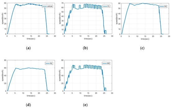
Figure 1.
Class 7 training dataset: (a) Vehicle speed; (b) Front left wheel speed; (c) Front right wheel speed; (d) Rear left wheel speed; (e) Rear right wheel speed.
In the case of validation data, we make attacks happen on four wheel speed sensors randomly at every moment and reduce the frequency of occurrence of attacks to 10 times since there exist only 5 sets. Figure 2 presents attacks in a validation dataset. The attack injection of test data is explained in Section 4.
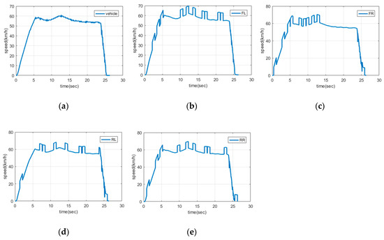
Figure 2.
Validation dataset: (a) Vehicle speed; (b) Front left wheel speed; (c) Front right wheel speed; (d) Rear left wheel speed; (e) Rear right wheel speed.
2.2. Recurrent Neural Network Architecture
RNN considers present information with historical information. RNN knows a current state of a system by checking time series data. A RNN architecture which is well designed enables a RNN classifier to differentiate attacked sensor data from normal sensor data correctly.
There are some parameters in architectures. We change one parameter while other parameters are fixed. While the parameters are changing, we choose the parameter when the result is the best experimentally. Firstly, the number of layers has to be selected to make an architecture. After the number of layers is fixed, the architecture is selected by comparing with RNN, Long Short-Term Memory (LSTM) and Gated Recurrent Unit (GRU) among DNNs [13,14]. Time step which DNNs consider as historical data is set to 90 by reference to [15]. Validation accuracy is checked with the fixed hyper-parameters. Table 2 shows the validation accuracy of each architecture depending on Neural Network (NN) models and the number of recurrent layers. Return sequences is a parameter term to decide whether that RNN layers maintain the number of a dimension same as time step in the output sequence. The access of a hidden state in a memory block of an RNN architecture relies on return sequences. Therefore, return sequences affects performances of RNN models, and it is important to set return sequences in the design of the architecture. The validation accuracy is the accuracy when a validation loss is the lowest among validation losses of epochs.
Table 2.
Some designed architectures to select the best architecture. LSTM: Long Short-Term Memory; GRU: Gated Recurrent Unit; RNN: Recurrent Neural Network.
In order to check the accuracies with fixed some parameters, return sequences first was set to true, and the number of recurrent layers was only changed. When the number of layers was two, the result was the best. The validation accuracy was more than 99% when the return sequences and the number of layers were modified to false and one, respectively. Therefore, the number of layers was not increased anymore. This is because the validation accuracy would not rise much from 99% although the calculation cost grows due to the growth of the number of layers.
We set hyper-parameters with Architecture 6 that shows the highest validation accuracy and uses RNN. In addition, the reason why to apply RNN is a simple situation where sensors are homogeneous, that is, there is no need to employ LSTM and GRU to have high computational complexity. Figure 3 presents Architecture 6 (bold) of RNN as shown in Table 2 in detail. In this work, features are each sensor data and input to RNN model like an image. , vector data of FL, FR, RL, and RR, is input as input data by 90 time steps. The input shape is (90, 4). The data passes the RNN layer which connects the previous information to the present information and are calculated at the Batch Normalization (BN) layer [16]. The number of neurons of the BN layer is equal to that of hidden neurons of RNN layer. Also, the number of neurons of the Softmax layer is the same as that of classes (15 in this work), and each neuron of Softmax layer calculates a probability of each class. Lastly, the architecture outputs a class number to have the highest probability. At a learning step, Adam is used as an optimizer and cross entropy is employed to calculate a loss [17].
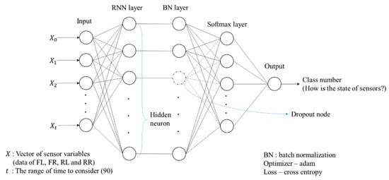
Figure 3.
Selected RNN architecture. BN: Batch Normalization.
2.3. Data Acquisition
In a proving ground of Korea Intelligent Automotive parts Promotion Institute (KIAPI), we drove Hyundai Motor’s Avante MD to acquire experimental data. The distance of the proving ground is 400 meters, and the vehicle was driven straight. A driver fully stamps down on the pedal of the accelerator until the vehicle reaches 60 km/h, which is the speed limit in two-lane urban roads. If the vehicle arrives beside a traffic cone, it is stopped by stepping on the brake pedal fully. Twenty-five datasets are gathered through 25 trials. They are separated into 15, 5, and 5 sets for training, validation, and testing, respectively. The training datasets are employed to be learned in RNN models and set both weighted values and threshold values of vehicle speed estimation algorithms. The validation datasets are exploited to validate a trained RNN model and tune hyper-parameters of the RNN model. We obtain the four wheel speed, brake pressure, and vehicle velocity data from CAN messages at 100 Hz using OBD-II. Vehicle velocities are generally calculated based on the four wheel speed data. Unfortunately, we only know final vehicle velocities calculated as Hyundai Motor does not release its own calculation algorithm for the vehicle velocities. In addition, obtained wheel speed data are expressed to the third decimal place, while vehicle velocity data are displayed as an integer only. Therefore, there are some errors between the final vehicle velocity data and the wheel speed data which are input to our algorithm as shown in Figure 4. We ignore these errors and compare how well our system estimates the vehicle speed with other algorithms.
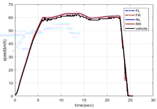
Figure 4.
Plotting wheel speed and vehicle speed data.
2.4. Hyper-Parameters
If hyper-parameters are set well, the accuracy of the model could increase. ReLu to represent nonlinearity and avoid vanishing gradient is chosen [18]. The number of hidden neurons is randomized from 1 to 90 and optimization of a batch size of input data, dropout probability, and learning rate is performed by a greedy search. Batch size {16, 32, 64, 128, 256} and learning rate {1e-5, 1e-4, 1e-3, 1e-2, 1e-1} are considered randomly. Dropout probability is adjusted from 0 to 1 by 0.1 interval [19]. Epoch is fixed to 30. Hyper-parameters are selected as optimal hyper-parameters when validation loss is the lowest after 100 searches. Table 3 shows the selected hyper-parameters.
Table 3.
Hyper-parameters setting.
3. Vehicle Speed Estimation
This section introduces the process of vehicle speed estimation using only data of normal sensors and excluding data of attacked sensors when attacks occur on sensors. Along with our proposed algorithm, other algorithms for performance comparison are explained. Weight and threshold values of the algorithms are set for the optimal speed estimation.
3.1. Fusion Algorithms
In this work, there are Recursive Filter (RF), Threshold Voting (TH), and WA in fundamental fusion algorithms. These three algorithms are the most fundamental sensor fusion algorithms using homogeneous sensors. As we employ four homogeneous wheel speed sensors, we check the results when the three algorithms are applied to estimate the vehicle speed. RF calculates precisely the present estimated values by reflecting the past estimated values. The equation of RF is as follows:
where is the estimated vehicle speed at time and is the merged sensor values by average at time . is a weight of RF, and the range of it is .
TF includes a sensor value for average calculation unless the distance between the sensor values is greater than a fixed threshold denoted as . The formula of TF is as below:
where ( is a value of wheel speed sensor (FL, FR, RL, RR) and is the difference between and .
WA calculates an average by assigning different weights to each sensor data. WA is expressed as follows:
where is the estimated vehicle speed at time and is a value of sensor at time . is a weight of sensor and the sum of all values of is 1. n is the total number of sensors considered in the calculation.
3.2. Weight and Threshold Selection
We find optimal weights and threshold values for the fusion algorithms, based on Mean Squared Error (MSE). We explain a method to determine the weight and threshold values used for each algorithm and focus on how to assign weights of WA depending on each class and driving condition (i.e., traction and braking). WA among fusion algorithms is modified for vehicle speed estimation because it is an algorithm which has an ability to adjust separately each weight of sensors depending on situations. Raw training datasets before injecting false data are exploited to set weights and thresholds.
A weight of RF is adjusted. When is 0.2, MSE is the lowest at 1.671 as presented in Table 4. The bold number means that we select the parameter and MSE value. Only normal data are used at this step, and data of attacked sensors are not included in the average calculation at a prediction step.
Table 4.
Weight selection of Recursive Filter.
In TV, the highest value among differences between data of two sensors is selected as a threshold in TV. Since the data pattern of traction differs from that of braking, thresholds of traction and braking are separately set. Table 5 presents the selected threshold values. In order to estimate the vehicle speed, in the case of attack occurrence, data of attacked sensors are excluded from the calculation, and only data of normal sensors are merged like RF.
Table 5.
Threshold selection of Threshold Voting.
We propose the two strategies to assign weights to WA. First, considering the driving condition, we reduce four individual weights used for FL, FR, RL, and RR to two weights for the front and rear wheels, and then find optimal values. In our experiment, the driving situation can be also divided into traction and braking since our scenario is to brake after going straight. Hence, the two front wheels move at the same speed and the pair of rear wheels also move concurrently with the same speed while the speeds of the front and rear wheels are different for each braking and traction. The same weight is assigned to the front wheels such as FR and FL, and a weight of RL is also equal to that of RR.
Second, considering the defined classes, the different weight is assigned to each sensor since each class has a different state. In the case of Class 0 (all the wheel speed sensors is in normal), weights are changed depending on traction and braking situation as shown in Table 6. The bold numbers are selected numbers as optimal weights and MSE. The meaning of bold number in Table 7 and 8 is also equal to that of the bold numbers in Table 6. If a current situation is a traction, weights of only rear sensors are increased. Otherwise, weights of only front sensors are increased. For example, if data of the wheel speed sensors is input, and a RNN classifier classifies a current state as Class 0, our system determines whether the operation of the system is in a braking situation or traction situation based on brake pedal data. If a driving condition is braking, each data of FL and FR is multiplied by 0.44 and each data of RL and RR is multiplied by 0.06 in the modified WA. Table 7 shows weights in case of Class 1 and 2 (only one of the front wheel speed sensors is attacked). Weights of both FL and FR are 0 and those of both RL and RR are 0.5 during traction when a state of the sensors is classified into Class 0 or 1. When a front wheel speed sensor is attacked during braking, a weight of FR or FL is 0.9, which is the high value, and weights of both RL and RR are 0.05. As presented in Table 8, the different weights are selected in case of Class 3 and 4 (only one of the rear wheel speed sensors is attacked). The vehicle speed is calculated by weighting only rear wheel speed sensors during traction where both front wheel speed sensors are in normal.
Table 6.
Weight selection of Weighted Average in Class 0 state.
Table 7.
Weight selection of Weighted Average in Class 1 and 2 states.
Table 8.
Weight selection of Weighted Average in Class 3 and 4 states.
By using weights of total classes as presented in Table 9, WA estimates the vehicle speed with the different weights depending on the traction and braking condition. Class 6, 7, 8, and 9 indicate that one of the front sensors and one of the rear sensors are attacked. The ratio of front weights to rear weights in Class 6, 7, 8, and 9 are equal to those of front weights to rear weights in Class 3 and 4 and Class 1 and 2. In other words, since one of the front sensors and one of the rear sensors are in normal, weights in Class 6, 7, 8, and 9 are as twice as weights in a state where all of the sensors are in normal. Because Class 5 and 10 mean that all front sensors or all rear sensors are in normal, 0.5 is assigned as the weight of each normal sensor. Class 11, 12, 13, and 14 indicate that only one of the four sensors is in normal. In this case, data of one sensor under normal operation become a vehicle speed.
Table 9.
Selected weights of Weighted Average in total classes.
4. Experimental Results
For the evaluation of the performance of sensor attack detection and vehicle speed estimation, the test datasets are used to test and analyze results in this section. The test datasets are different from the experimental datasets before. Test accuracies are calculated for performance evaluation of RNN classifier for attack detection. In case of speed estimation, we discuss MSE results of RF, TV, and WA.
4.1. Classification Accuracy
In order to generate a test environment, we design the parameters such as attack duration, timing which attacks occur in test datasets. All of the five test datasets followed the Poisson distribution and the Poisson mean is set to 0.1 (the average number of events per one second). The Poisson distribution is a probability distribution that indicates the occurrence frequency of events. The occurrence frequency of attacks is depend on the mind of the attacker. Thus, Poisson distribution is suitable for expressing occurrence of attacks randomly and was used for attack data generation. Attack duration is fixed to 0.73 and a type of attack is limited to additive attack as well as random and drift attacks.
The accuracy is a measure to show how well states of the wheel speed sensors are classified before calculating the vehicle speed. We check the accuracy by inputting the test data as input data of the RNN classifier. It is necessary to ensure high classification accuracy in that only the data of the normal sensors are used for vehicle speed estimation. The accuracy is 99.4978% when the test datasets are classified by the trained RNN classifier.
There are some misclassified data, and we analyze them in order to identify the cause. Figure 5 shows the misclassified data in one of five test datasets. Figure 5a presents the profile of the data input to the RNN classifier after attack injection. Figure 5b illustrates the reference speed obtained from CAN to check that the attack is classified well and the estimated speed after attack detection and speed estimation. The enlargements of each green box of Figure 5a,b are displayed in Figure 5c,d. As shown in Figure 5c,d, data that the green circles indicate are misclassified as false data in spite of data of a normal sensor. The wheel speed value is momentarily higher than the vehicle speed because the four wheels are tightened by disc pads and locked, and then the wheel speeds are compensated by Proportional–Integral–Derivative (PID) control after ABS operation [20]. At that moment, the confusion arises in the classification process.
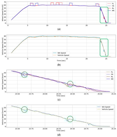
Figure 5.
One of the test datasets: (a) Test dataset before attack detection; (b) The estimated speed after attack detection and speed estimation and the reference speed; (c) A part of the test dataset before attack detection; (d) A part of the estimated speed after attack detection and speed estimation and the reference speed.
On the contrary, although an attack happens on a sensor, there is a result that the RNN classifier predicted as a normal state. Another test dataset is presented in Figure 6. Figure 6a,b show total profiles of the dataset. Data to inject false data into and input to the RNN classifier for attack detection are illustrated in Figure 6a. The reference speed and the estimated speed which WA calculates after attack detection are displayed in Figure 6b. In Figure 6c,d, the green boxes of Figure 6a,b are enlarged, respectively. The green circle indicates that the RNN classifier misclassified the class of the data as a normal operation though an attack occurred on a sensor as shown in Figure 6c,d. This is because the magnitude of the data is smaller than that of other false data.
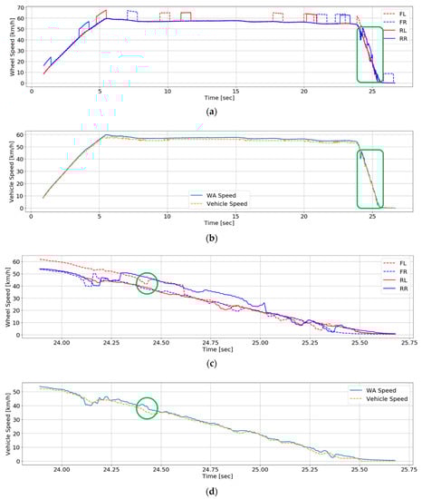
Figure 6.
Another test dataset: (a) Test dataset before attack detection; (b) The estimated speed after attack detection and speed estimation and the reference speed; (c) A part of the test dataset before attack detection; (d) A part of the test dataset after attack detection and speed estimation.
The data of normal sensors and attacked sensors on which additional attacks happen are learned at the learning step. Note that other types of sensor attacks are considered to know what the results show when unlearned data of sensor attacks are input. Random attacks and drift attacks are generated with the same test data used for additional attacks. A random value is added to a sensor value for generating a random attack. The equation of random attacks is written as below:
where and is equal to the notations of an additive attack. is a random value to follow uniform distribution from 0 to defined in the additive attack.
Drift attacks linearly increase a value added to a sensor value. The drift attacks are calculated as follows:
where , and are same as the notations of an additive attack. is the time when a drift attack is introduced, is the duration of the ramp (0.73 second).
We made 15 test datasets that three types of attacks are injected into with the same test datasets. As presented in Figure 7a,c,e, the range and time of the attack occurrence of three types are identical in the three datasets. Table 10 displays test accuracies about each attack. As mentioned before, the accuracy about the total test data of additional attacks is 99.4978%. Test accuracies about those of random attacks and drift attacks are 86.1985% and 86.5594%, respectively. The results show about 23% lower probability than the test accuracy of additional attacks. Figure 7b,d,f shows how correctly WA estimates the vehicle speed by classifying each attacked and normal sensors in the test datasets. While WA estimates the relatively the correct vehicle speed after attack detection with the data of Figure 7a as presented in Figure 7b, the false data to have small magnitude are not processed after attack detection and speed estimation with each data of Figure 7c,e as shown in Figure 7d,f. The RNN classifier detects and identifies only false data to have large magnitude like additional attacks as it learned data of additional attacks. It is needed to process the pattern of unlearned data to increase the accuracies about random attacks and drift attacks over 90% as future work.
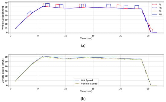
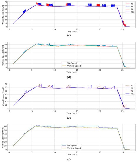
Figure 7.
Datasets inject false data: (a) Four wheel speed data to consider additive attacks; (b) Estimated speed against additive attacks and reference speed data; (c) Four wheel speed data to consider random attacks (d) Estimated speed against random attacks and reference speed data; (e) Four wheel speed data to consider drift attacks; (f) Estimated speed against drift attacks and reference speed data.
Table 10.
Test accuracies.
4.2. Mean Squared Error
MSE can be generally used to investigate how accurately fusion algorithms calculate vehicle speeds. When the experiment is performed with test datasets of additional attack, MSEs of RF, TV, and WA are 1.904, 1.9089, and 1.7786, respectively (see Table 11). WA shows the lowest MSE among the algorithms. Since there are differences between the raw wheel speed data and the vehicle speed data as mentioned in Section 2, there also exist differences between the speed data estimated based on the wheel speed data and vehicle speed data.
Table 11.
Mean squared error (MSE).
The reference vehicle speed and the vehicle speed estimated by the fusion algorithms during acceleration are illustrated in Figure 8a. The reference vehicle speed is plotted as stairs since Hyundai Motor provides the vehicle speed as only integer number via CAN. Figure 8b displays the enlarged part of the purple box in Figure 8a. Before 3.3 seconds there is no difference between performances of the algorithms, but after 3.3 seconds WA estimates the vehicle speed more closely. The vehicle speed and the wheel speed input to our system to explain the cause in the same range of Figure 8b are presented in Figure 8c. Attacks occur on RR and RL before 3.3 seconds while attacks happen on only RL after 3.3 seconds. As all of the three algorithms calculate average except data of sensors on which attacks occur, they are the same before 3.3 seconds. In case of WA after 3.3 seconds, the average is calculated by assigning high weights of rear sensors. Therefore, WA speed is calculated close to RR data.
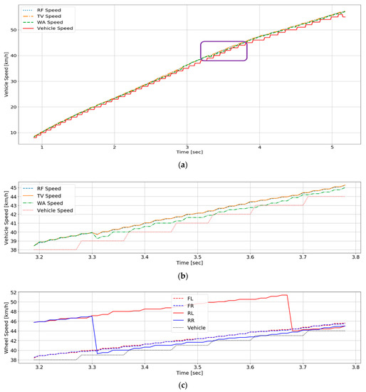
Figure 8.
Comparison of fusion algorithms during acceleration: (a) Acceleration; (b) Vehicle speed and estimated speed; (c) Vehicle speed and wheel speed to inject false data into.
Figure 9a shows the reference speed and the speed estimated by the fusion algorithms while the vehicle speed is kept close to constant speed. Figure 9b illustrates the enlarged part of the purple box in Figure 9a. It is difficult to find differences between performances of the algorithms as the vehicle maintains the vehicle speed. We can see that the reference speed goes back and forth between 58 and 59 km/h and is represented as the only integer. Hence, the integer 1 km/h seems to change if 0.01 km/h, which is a specific decimal, changes.
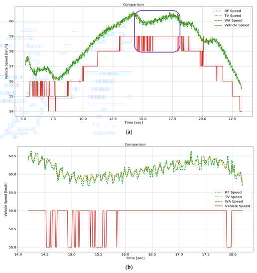
Figure 9.
Comparison of fusion algorithms during constant speed: (a) Constant speed; (b) Vehicle speed and estimated speed.
The reference speed and the speed estimated by the fusion algorithms during braking are displayed in Figure 10a. Figure 10b presents an enlarged part of the purple box in Figure 10a. The speed estimated by RF and TV is similar, but WA shows a closer estimation of vehicle speed. Wheel speed data for result analysis are shown in Figure 10c. All wheel speed sensors are in normal operation, and the data of FR and FL are actually close to the vehicle speed data. MSE of WA is lower than those of RF and TV because WA estimates vehicle speed by much weighting the front sensors during braking. Thus, WA, which assigns different weights depending on a situation, is safer than other algorithms in terms of handling data integrity. WA was applied with data of a sedan car in this paper. Further research is needed to make a system applicable to vehicles to have different data patterns.
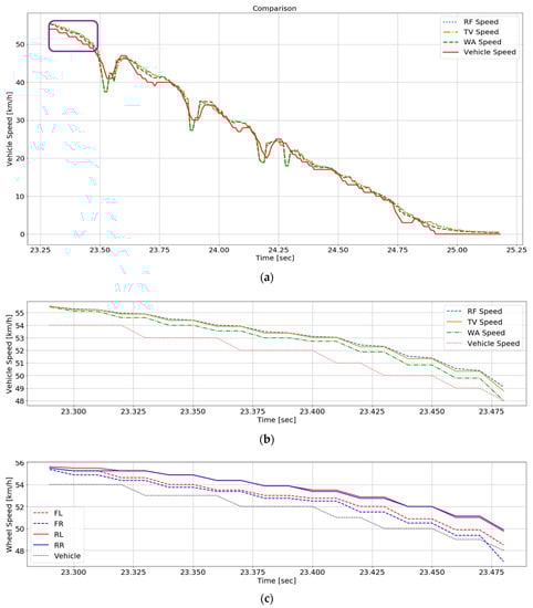
Figure 10.
Comparison of fusion algorithms during braking: (a) Braking; (b) Vehicle speed and estimated speed; (c) Vehicle speed and wheel speed to inject false data into.
5. Conclusions
This paper described the sensor attack detection and vehicle speed estimation method. The sensor attack detection method to use RNN was suggested and it focuses on the wheel speed sensors. The vehicle speed estimation method without an additional sensor is studied for data integrity of the wheel speed sensors. We firstly defined classes and divided a driving situation into traction and braking. WA to calculate different weighted values of wheels relying on the classes and situations was applied in the vehicle speed estimation. Attack detection and identification were performed with a high probability, and MSE of the proposed system was lower than those of other algorithms. Attack detection and identification is a necessary process since vehicle speed is calculated with only normal data. The high classification accuracy is required to correctly estimate the vehicle speed. Moreover, the modified WA to show the lowest MSE has relatively high integrity. In other words, exact speed information means high integrity. It turned out that the system used the modified WA is safe because high integrity is related to the life of drivers and pedestrians.
Our system is applicable to a diagnosis system in CPS. If the diagnosis system is applied when an attack occurs on the wheel speed sensors in automotive CPS, the estimated vehicle speed information instead of vehicle speed calculated with the false wheel speed data will be transmitted to a controller. The controller may control the vehicle based on the information, and the system would contribute to the safety of drivers and pedestrians. In addition to wheel speed sensors of the vehicle, it is possible to apply our system to other sensors of the vehicle or sensors of other platforms. In the future, an online learning method is needed in case untrained data is input as new data. In addition, it is necessary to expand the system after experimenting with various environments including left and right turn and other road surfaces. We have a plan to investigate reinforcement learning and WA with not constant but adaptive weighted values to apply the proposed system to vehicles with different data patterns and overcome the above limitations.
Author Contributions
Conceptualization, J.S.; methodology, J.S.; software, J.S.; validation, J.S., Y.B.; formal analysis, J.S., Y.B., J.L. and S.L.; investigation, J.S. and Y.B..; resources, J.S., J.L and S.L.; data curation, J.S.; writing—original draft preparation, J.S. and Y.B.; writing—review and editing, J.S. and Y.B.; visualization, J.S.; supervision, J.S. and Y.B.; project administration, Y.B. and S.L.; funding acquisition, Y.B. and S.L.
Funding
This research was supported in part by Global Research Laboratory Program (Grant No.: 2013K1A1A2A02078326) through the NRF of Korea, DGIST Research and Development Program funded by the Ministry of Science, ICT and Future Planning (Grand No.: 18-IT-01), and Institute for Information & communications Technology Promotion (IITP) grant funded by the Korean government (MSIT) (No. 2014-0-00065, Resilient Cyber-Physical Systems Research).
Conflicts of Interest
The authors declare no conflict of interest.
References
- Rajkumar, R.; Lee, I.; Sha, L.; Stankovic, J. Cyber-physical systems: The next computing revolution. In Proceedings of the Design Automation Conference, Anaheim, CA, USA, 13–18 June 2010; pp. 731–736. [Google Scholar]
- Yan, R.; Ma, Z.; Kokogiannakis, G.; Zhao, Y. A sensor fault detection strategy for air handling units using cluster analysis. Autom. Constr. 2016, 70, 77–88. [Google Scholar] [CrossRef]
- Moon, T.Y.; Seo, S.H.; Kim, J.H.; Hwang, S.H.; Jeon, J.W. Gateway system with diagnostic function for LIN, CAN and FlexRay. In Proceedings of the International Conference on Control, Automation and Systems, Seoul, Korea, 17–20 October 2007; pp. 2844–2849. [Google Scholar]
- Kwon, C.; Liu, W.; Hwang, I. Security analysis for cyber-physical systems against stealthy deception attacks. In Proceedings of the American Control Conference, Washington, DC, USA, 17–19 June 2013; pp. 3344–3349. [Google Scholar]
- Park, J.; Ivanov, R.; Weimer, J.; Pajic, M.; Lee, I. Sensor attack detection in the presence of transient faults. In Proceedings of the ACM/IEEE Sixth International Conference on Cyber-Physical Systems, New York, NY, USA, 14–16 April 2015; pp. 1–10. [Google Scholar]
- Samy, I.; Postlethwaite, I.; Gu, D.W. Detection and accommodation of sensor faults in UAVs-a comparison of NN and EKF based approaches. In Proceedings of the 49th IEEE Conference on Decision and Control, Atlanta, GA, USA, 15–17 December 2010; pp. 4365–4372. [Google Scholar]
- Amin, S.; Litrico, X.; Sastry, S.S.; Bayen, A.M. Cyber security of water SCADA systems—Part II: Attack detection using enhanced hydrodynamic models. IEEE Trans. Control Syst. Technol. 2013, 21, 1679–1693. [Google Scholar] [CrossRef]
- Lipton, Z.C.; Berkowitz, J.; Elkan, C. A critical review of recurrent neural networks for sequence learning. arXiv, 2015; arXiv:1506.00019. [Google Scholar]
- Song, C.K.; Uchanski, M.; Hedrick, J.K. Vehicle speed estimation using accelerometer and wheel speed measurements. SAE Int. 2002, 01, 2229. [Google Scholar]
- Bevly, D.M.; Gerdes, J.C.; Wilson, C. The use of GPS based velocity measurements for measurement of sideslip and wheel slip. Veh. Syst. Dyn. 2002, 38, 127–147. [Google Scholar]
- Blank, S.; Föhst, T.; Berns, K. A case study towards evaluation of redundant multi-sensor data fusion. In Proceedings of the Commercial Vehicle Technology, Kaiserslautern, Germany, 16–18 March 2010. [Google Scholar]
- Fitch, G.M.; Blanco, M.; Morgan, J.F.; Wharton, A.E. Driver braking performance to surprise and expected events. Proc. Hum. Ergo. SAGE. 2010, 54, 2075–2080. [Google Scholar] [CrossRef]
- Cho, K.; Van Merriënboer, B.; Gulcehre, C.; Bahdanau, D.; Bougares, F.; Schwenk, H.; Bengio, Y. Learning phrase representations using RNN encoder-decoder for statistical machine translation. arXiv, 2014; arXiv:1406.1078. [Google Scholar]
- Hochreiter, S.; Schmidhuber, J. Long short-term memory. Neural Comput. 1997, 9, 1735–1780. [Google Scholar] [CrossRef] [PubMed]
- Shin, J.; Baek, Y.; Eun, Y.; Son, S.H. Intelligent sensor attack detection and identification for automotive cyber-physical systems. In Proceedings of the 2017 IEEE Symposium Series on Computational Intelligence, Honolulu, HI, USA, 27 November–1 December 2017; pp. 1–8. [Google Scholar]
- Ioffe, S.; Szegedy, C. Batch normalization: Accelerating deep network training by reducing internal covariate shift. arXiv, 2015; arXiv:1502.03167. [Google Scholar]
- Kingma, D.P.; Ba, J. Adam: A method for stochastic optimization. arXiv, 2014; arXiv:1412.6980. [Google Scholar]
- Nair, V.; Hinton, G.E. Rectified linear units improve restricted boltzmann machines. In Proceedings of the 27th international conference on machine learning, Haifa, Israel, 21–24 June 2010; pp. 807–814. [Google Scholar]
- Srivastava, N.; Hinton, G.; Krizhevsky, A.; Sutskever, I.; Salakhutdinov, R. Dropout: A simple way to prevent neural networks from overfitting. J. Mach. Learn. Res. 2014, 15, 1929–1958. [Google Scholar]
- Aly, A.A.; Zeidan, E.S.; Hamed, A.; Salem, F. An antilock-braking systems (ABS) control: A technical review. Intell. Control Autom. 2011, 2, 186–195. [Google Scholar] [CrossRef]


© 2018 by the authors. Licensee MDPI, Basel, Switzerland. This article is an open access article distributed under the terms and conditions of the Creative Commons Attribution (CC BY) license (http://creativecommons.org/licenses/by/4.0/).